

On the Influence of Aging on Classification Performance in the Visual EEG Oddball Paradigm Using Statistical and Temporal Features
 , , , and
Abstract
:1. Introduction
Related Work
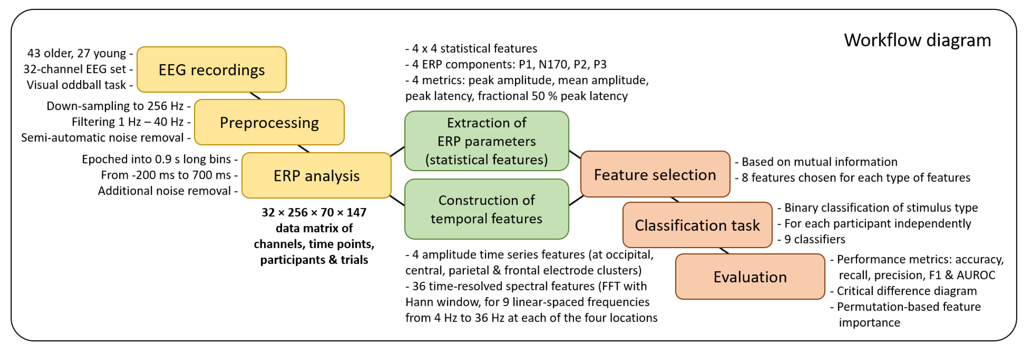
2. Methods
2.1. Participants
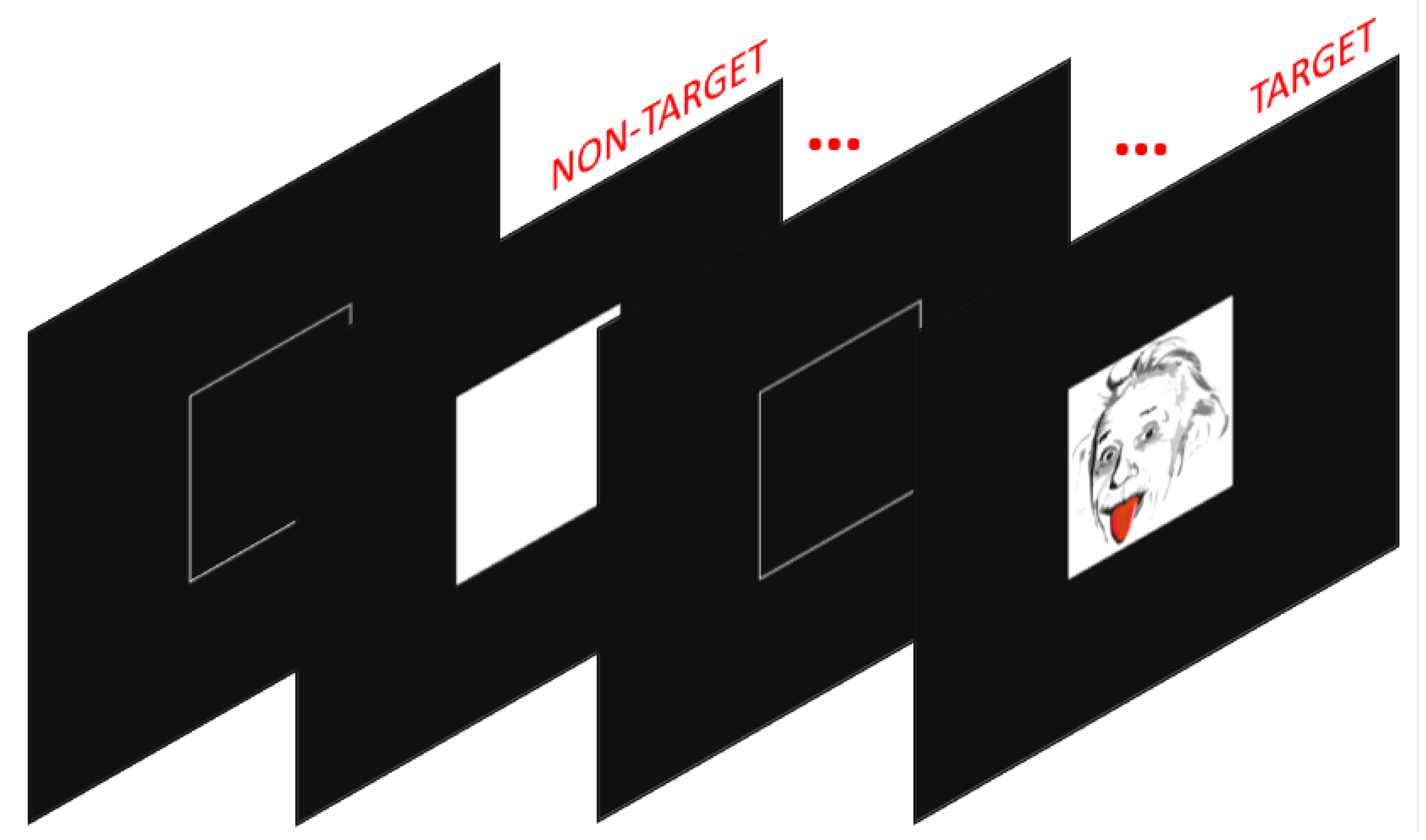
2.2. Visual Oddball Task
2.3. EEG Analysis
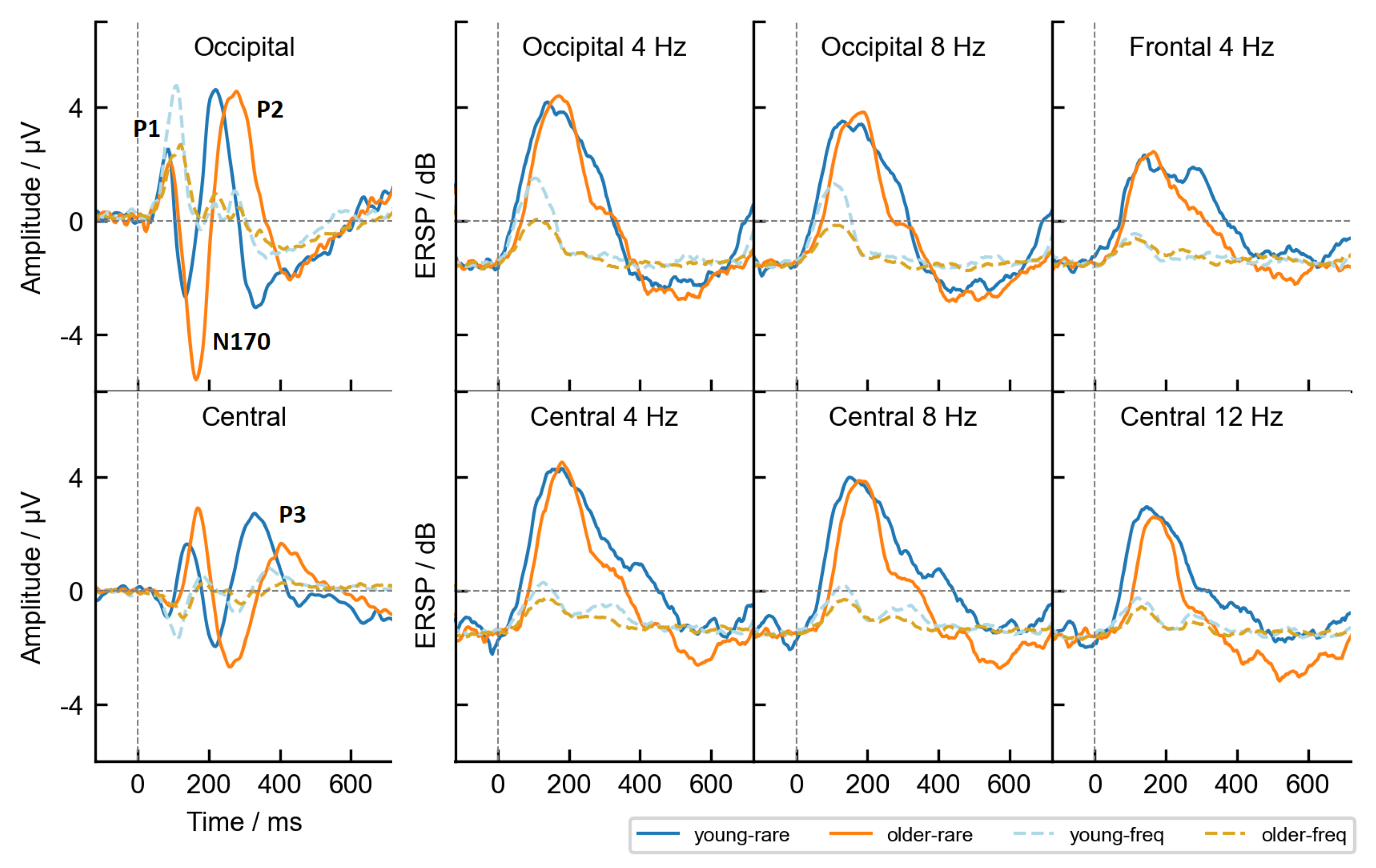
2.4. ERP Analysis
2.5. Extraction of Temporal Features
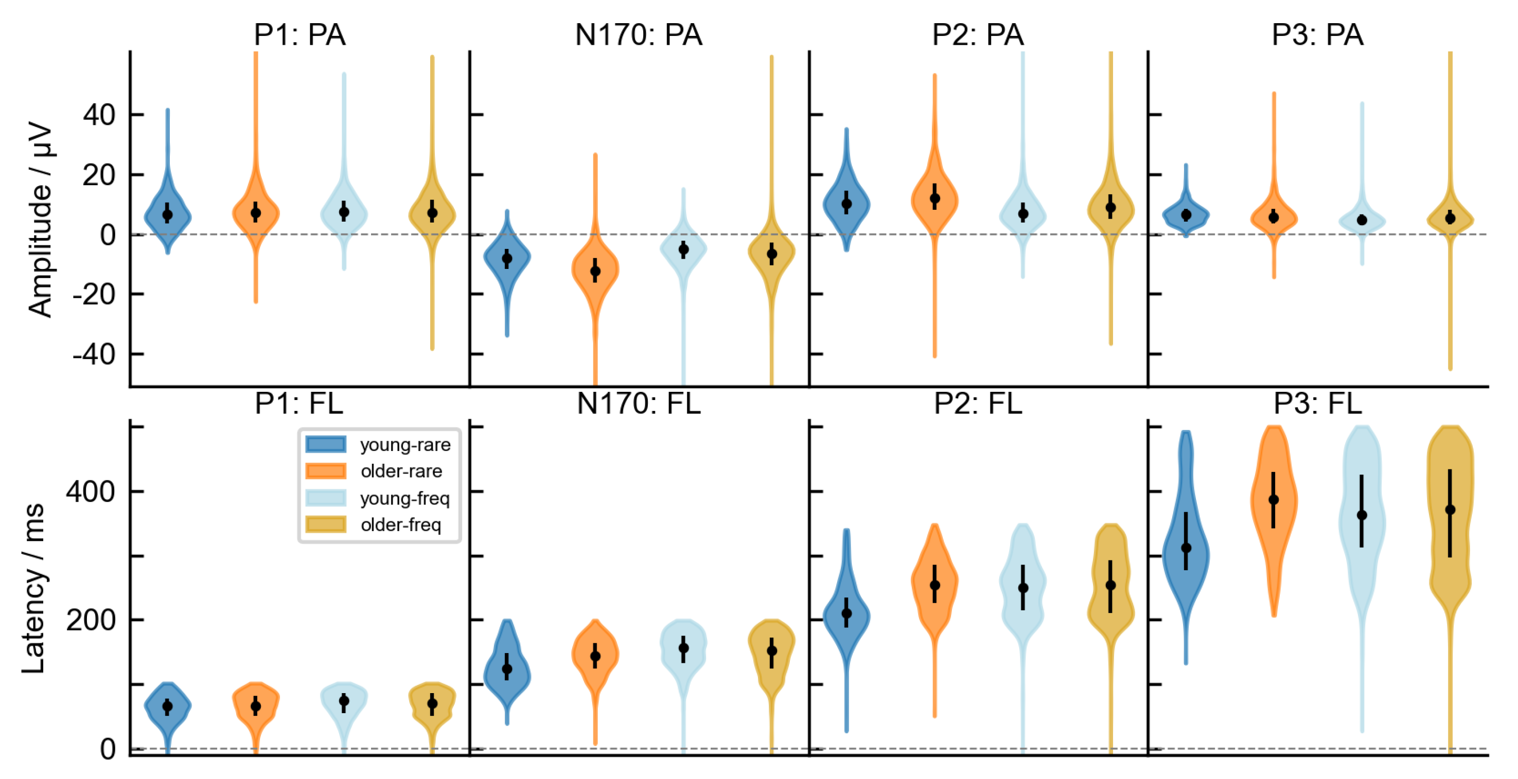
2.6. Extraction of Time-Independent Statistical ERP Features
2.7. Classification Task
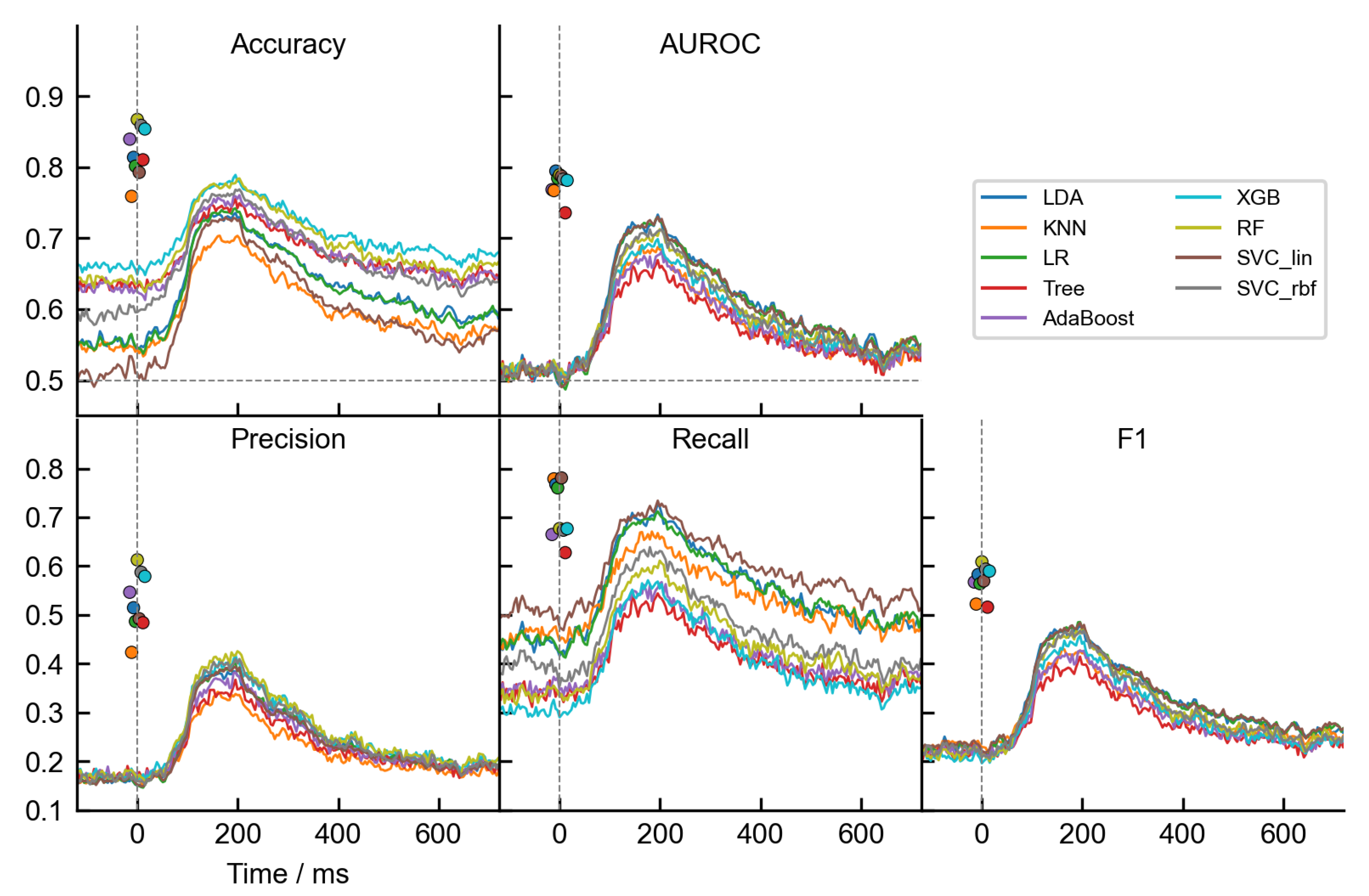
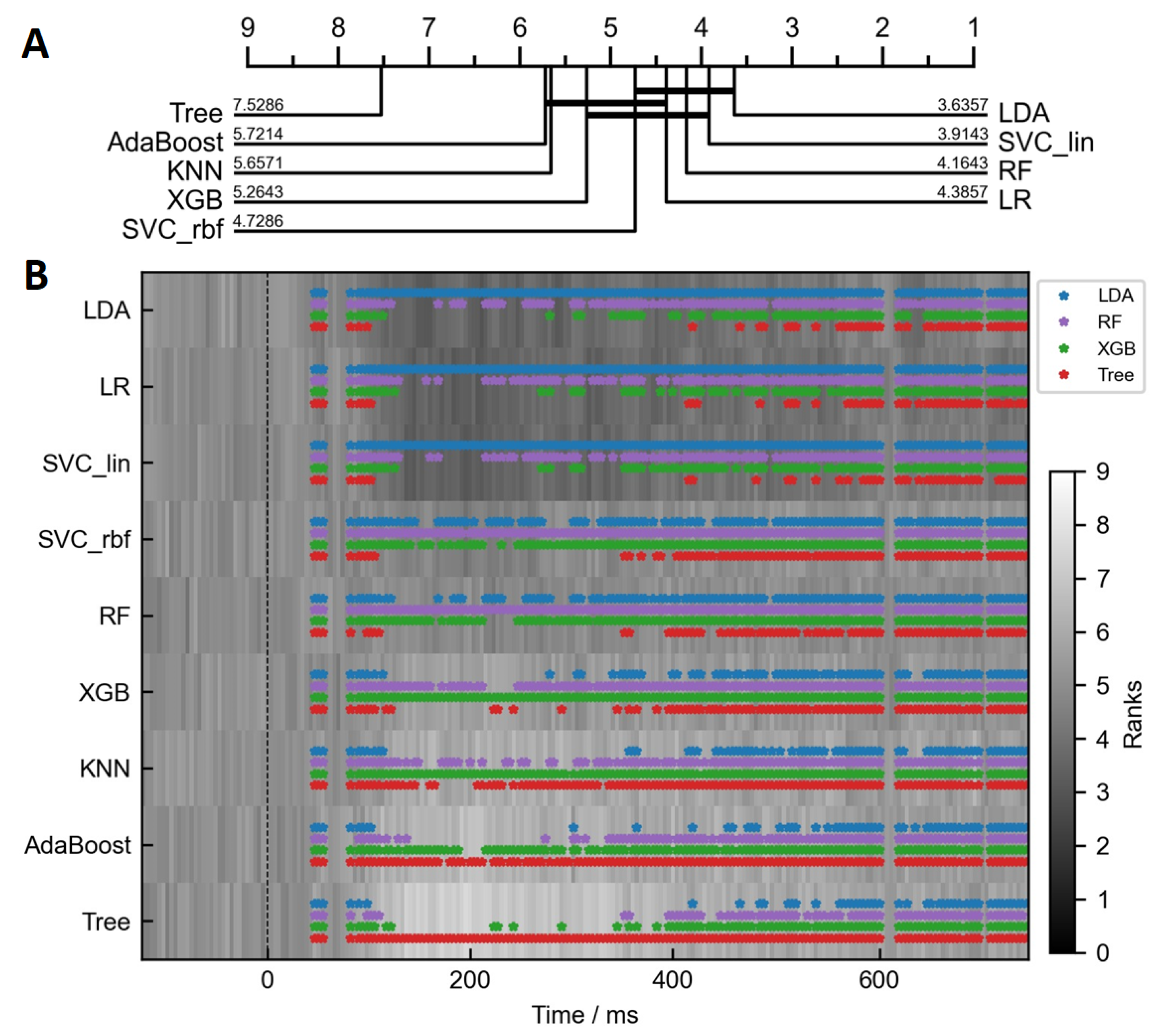
3. Results
3.1. Differences between Classifiers
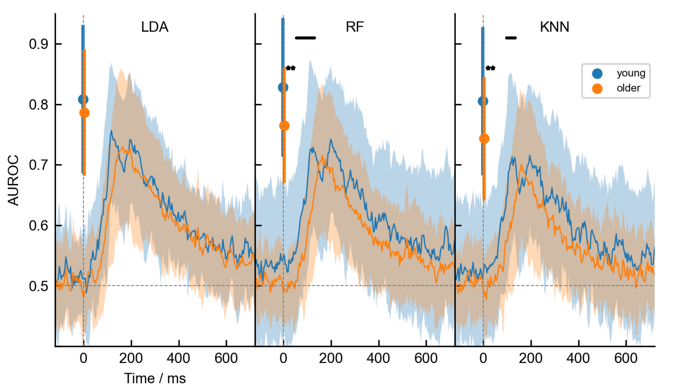
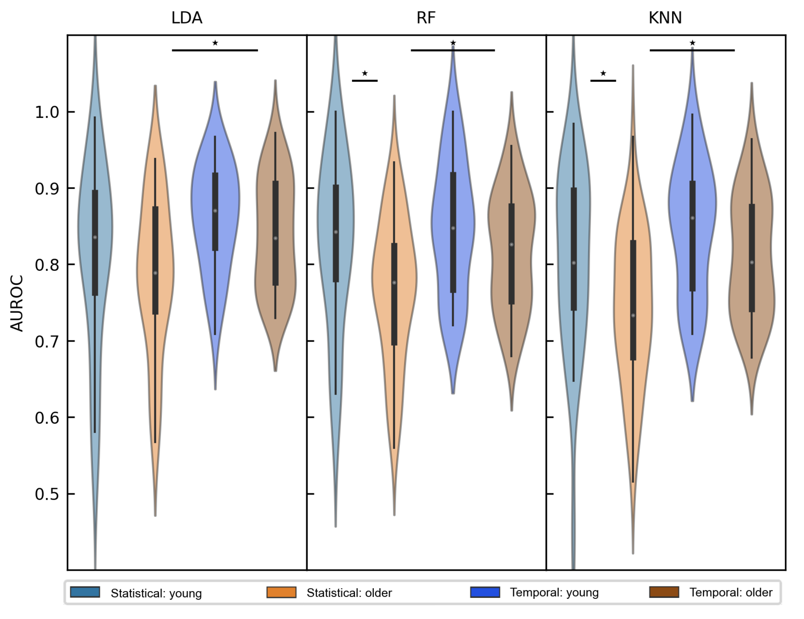
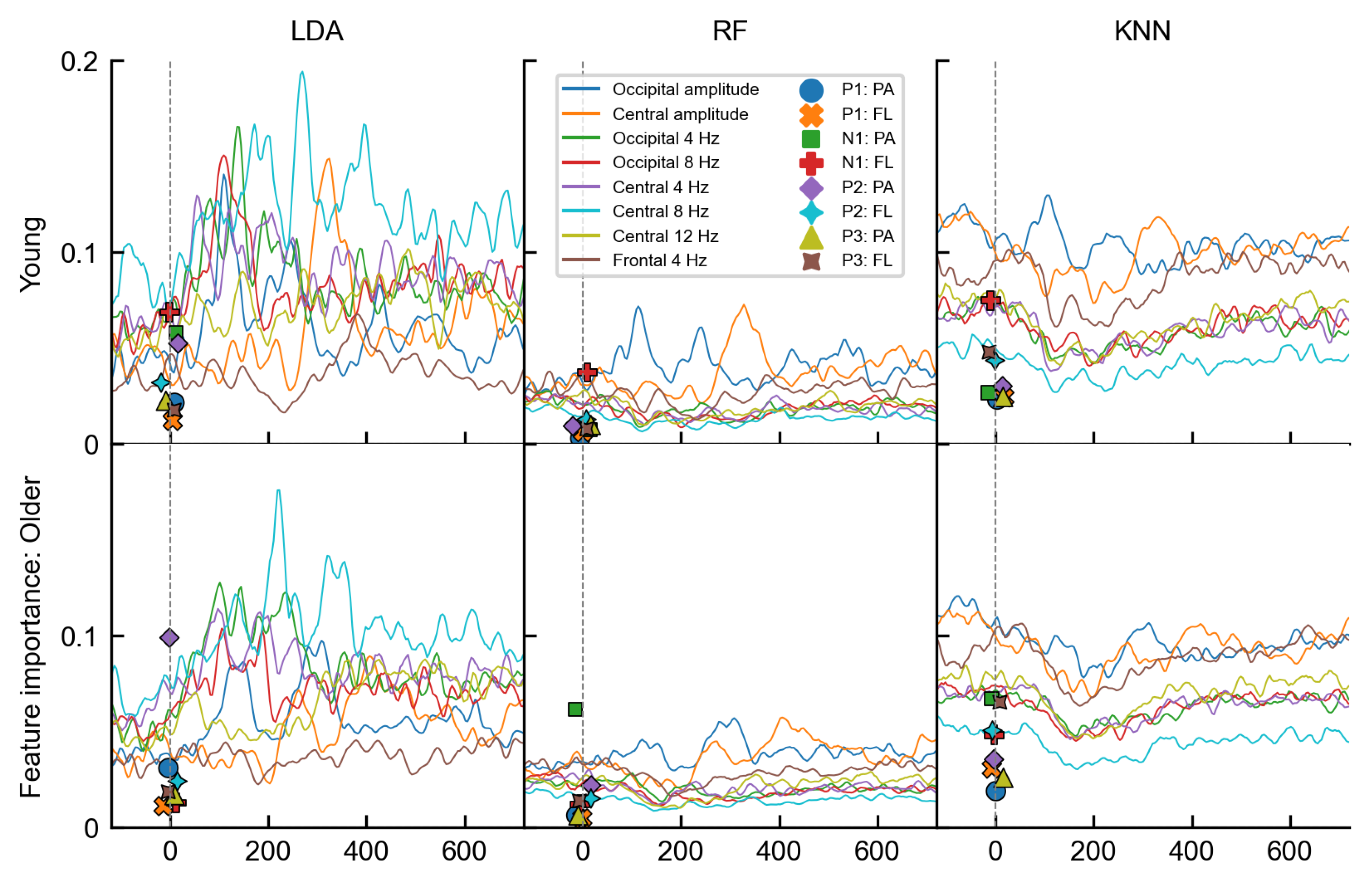
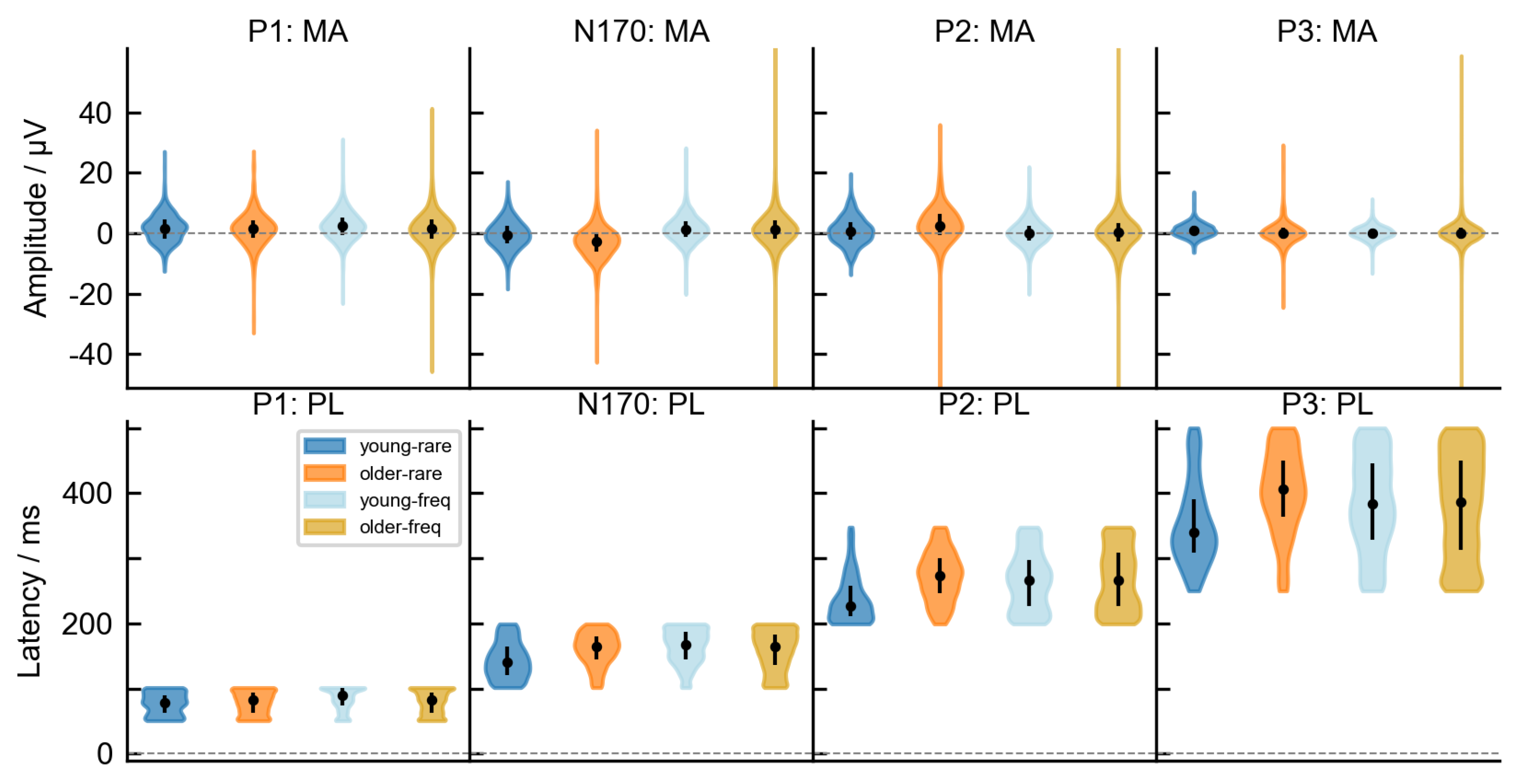
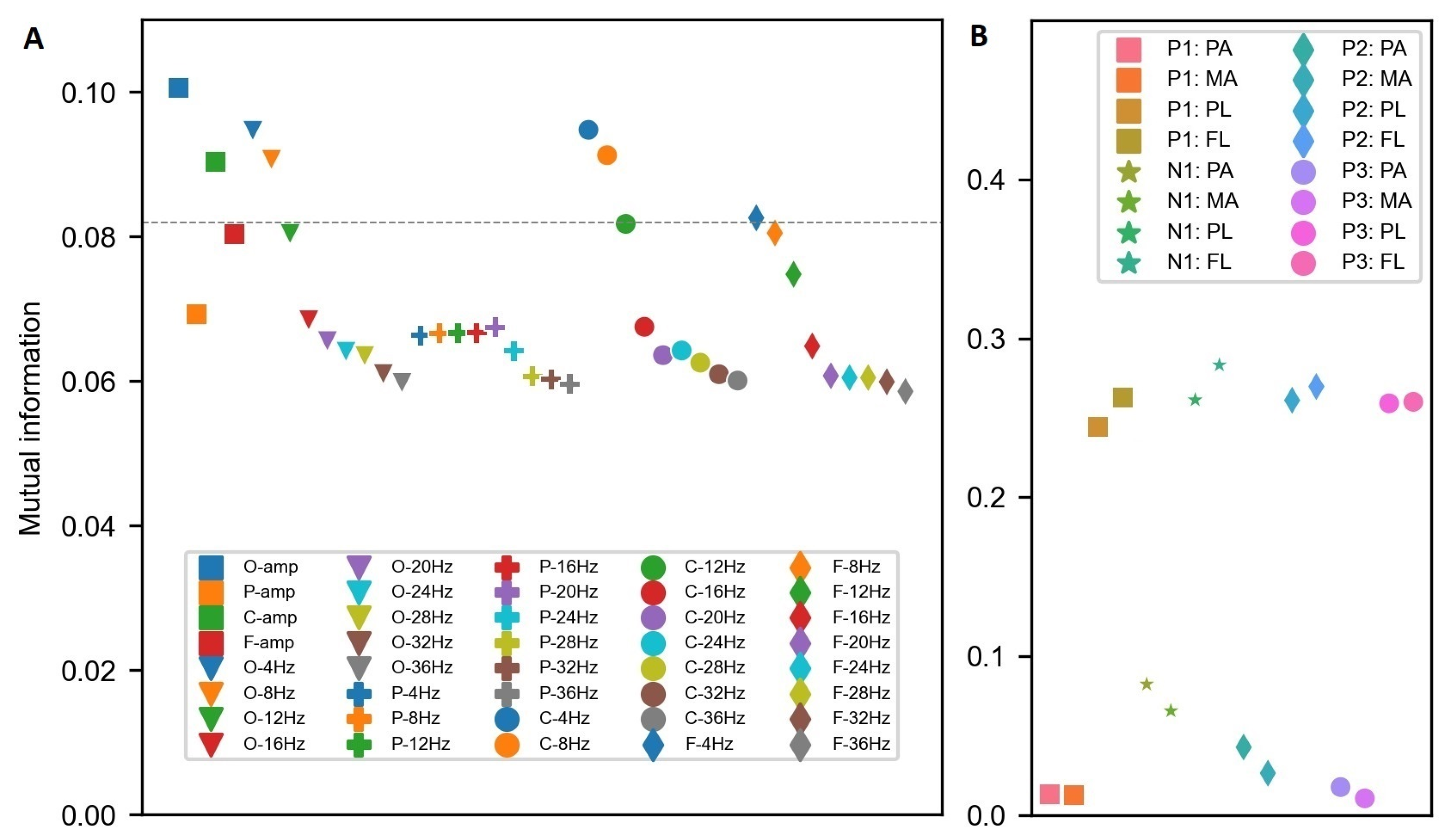
3.2. Age-Related Differences
4. Discussion
Author Contributions
Funding
Institutional Review Board Statement
Informed Consent Statement
Data Availability Statement
Acknowledgments
Conflicts of Interest
Abbreviations
| AUROC | Area under the receiver operating curve |
| BCI | Brain-computer interfaces |
| EEG | Electroencephalogram |
| ERP | Event-related potential |
| ERSP | Event-related spectral perturbation |
| FN | False negative |
| FP | False positive |
| FPR | False positive rate |
| FL | Fractional 50% peak latency |
| LDA | Linear discriminant analysis |
| LR | Linear regression |
| KNN | K-Nearest neighbors |
| MA | Mean amplitude |
| MCI | Mild cognitive impairment |
| PA | Peak amplitude |
| PL | Peak latency |
| RF | Random forest |
| SVC | Support vector machine |
| TN | True negative |
| TP | True positive |
| TPR | True positive rate |
| XGB | Extreme Gradient Boosting |
Appendix A

Appendix B
Appendix C
Appendix D

References
- Rashid, M.; Sulaiman, N.; Majeed, A.P.P.A.; Musa, R.M.; Nasir, A.F.A.; Bari, B.S.; Khatun, S. Current status, challenges, and possible solutions of EEG-based brain-computer interface: A comprehensive review. Front. Neurorobot. 2020, 14, 25. [Google Scholar] [CrossRef]
- Breakspear, M. Dynamic models of large-scale brain activity. Nat. Neurosci. 2017, 20, 340–352. [Google Scholar] [CrossRef]
- Ghorbanian, P.; Ramakrishnan, S.; Ashrafiuon, H. Stochastic non-linear oscillator models of EEG: The alzheimer’s disease case. Front. Comput. Neurosci. 2015, 9, 48. [Google Scholar] [CrossRef] [PubMed] [Green Version]
- Miladinović, A.; Ajčević, M.; Jarmolowska, J.; Marusic, U.; Colussi, M.; Silveri, G.; Battaglini, P.P.; Accardo, A. Effect of power feature covariance shift on BCI spatial-filtering techniques: A comparative study. Comput. Methods Prog. Biomed. 2021, 198, 105808. [Google Scholar] [CrossRef]
- Wolpaw, J.R.; Birbaumer, N.; McFarland, D.J.; Pfurtscheller, G.; Vaughan, T.M. Brain-computer interfaces for communication and control. Clin. Neurophysiol. Off. J. Int. Fed. Clin. Neurophysiol. 2002, 113, 767–791. [Google Scholar] [CrossRef]
- Lotte, F.; Bougrain, L.; Cichocki, A.; Clerc, M.; Congedo, M.; Rakotomamonjy, A.; Yger, F. A review of classification algorithms for EEG-based brain–computer interfaces: A 10 year update. J. Neural Eng. 2018, 15, 031005. [Google Scholar] [CrossRef] [Green Version]
- Bamdad, M.; Zarshenas, H.; Auais, M.A. Application of BCI systems in neurorehabilitation: A scoping review. Disabil. Rehabil. Assist. Technol. 2015, 10, 355–364. [Google Scholar] [CrossRef]
- Aggarwal, S.; Chugh, N. Review of machine learning techniques for EEG based brain computer interface. Arch. Comput. Methods Eng. 2022, 29, 3001–3020. [Google Scholar] [CrossRef]
- Luck, S.J. Event-Related Potentials; American Psychological Association: Washington, DC, USA, 2012. [Google Scholar]
- Daniel, S.; Bentin, S. Age-related changes in processing faces from detection to identification: ERP evidence. Neurobiol. Aging 2012, 33, 206.e1–206.e28. [Google Scholar] [CrossRef] [Green Version]
- Luck, S.J. An Introduction to the Event-Related Potential Technique, 2nd ed.; The MIT Press: Cambridge, MA, USA, 2014; p. 416. [Google Scholar]
- Dustman, R.E.; Beck, E.C. The effects of maturation and aging on the wave form of visually evoked potentials. Electroencephalogr. Clin. Neurophysiol. 1969, 26, 2–11. [Google Scholar] [CrossRef]
- Polich, J. EEG and ERP assessment of normal aging. Electroencephalogr. Clin. Neurophysiol. Potentials Sect. 1997, 104, 244–256. [Google Scholar] [CrossRef] [PubMed]
- Grady, C.L. Cognitive neuroscience of aging. Ann. N. Y. Acad. Sci. 2008, 1124, 127–144. [Google Scholar] [CrossRef] [PubMed] [Green Version]
- Anderson, A.J.; Perone, S. Developmental change in the resting state electroencephalogram: Insights into cognition and the brain. Brain Cogn. 2018, 126, 40–52. [Google Scholar] [CrossRef] [PubMed]
- Salthouse, T.A. The processing-speed theory of adult age differences in cognition. Psychol. Rev. 1996, 103, 403. [Google Scholar] [CrossRef] [Green Version]
- Vysata, O.; Kukal, J.; Prochazka, A.; Pazdera, L.; Valis, M. Age-related changes in the energy and spectral composition of EEG. Neurophysiology 2012, 44, 63–67. [Google Scholar] [CrossRef]
- Celesia, G.G.; Kaufman, D.; Cone, S. Effects of age and sex on pattern electroretinograms and visual evoked potentials. Electroencephalogr. Clin. Neurophysiol. Potentials Sect. 1987, 68, 161–171. [Google Scholar] [CrossRef]
- Mitchell, K.; Howe, J.; Spencer, S. Visual evoked potentials in the older population: Age and gender effects. Clin. Phys. Physiol. Meas. 1987, 8, 317. [Google Scholar] [CrossRef]
- Aleksić, P.; Raicević, R.; Stamenković, M.; Djordjević, D. Effect of aging on visual evoked potentials. Vojnosanit. Pregl. 2000, 57, 297–302. [Google Scholar]
- Kuba, M.; Kremláček, J.; Langrová, J.; Kubová, Z.; Szanyi, J.; Vít, F. Aging effect in pattern, motion and cognitive visual evoked potentials. Vis. Res. 2012, 62, 9–16. [Google Scholar] [CrossRef] [Green Version]
- Kropotov, J.; Ponomarev, V.; Tereshchenko, E.P.; Müller, A.; Jäncke, L. Effect of aging on ERP components of cognitive control. Front. Aging Neurosci. 2016, 8, 69. [Google Scholar] [CrossRef]
- Hsu, H.T.; Lee, I.H.; Tsai, H.T.; Chang, H.C.; Shyu, K.K.; Hsu, C.C.; Chang, H.H.; Yeh, T.K.; Chang, C.Y.; Lee, P.L. Evaluate the feasibility of using frontal SSVEP to implement an SSVEP-based BCI in young, elderly and ALS groups. IEEE Trans. Neural Syst. Rehabil. Eng. 2015, 24, 603–615. [Google Scholar] [CrossRef] [PubMed]
- Dias, N.; Mendes, P.; Correia, J. Subject age in P300 BCI. In Proceedings of the 2nd International IEEE EMBS Conference on Neural Engineering, Arlington, VA, USA, 16–19 March 2005; IEEE: New York, NY, USA, 2005; pp. 579–582. [Google Scholar]
- Park, D.C.; Reuter-Lorenz, P. The adaptive brain: Aging and neurocognitive scaffolding. Annu. Rev. Psychol. 2009, 60, 173. [Google Scholar] [CrossRef] [Green Version]
- Lotte, F.; Congedo, M.; Lécuyer, A.; Lamarche, F.; Arnaldi, B. A review of classification algorithms for EEG-based brain–computer interfaces. J. Neural Eng. 2007, 4, R1. [Google Scholar] [CrossRef] [PubMed] [Green Version]
- Stancin, I.; Cifrek, M.; Jovic, A. A Review of EEG Signal Features and Their Application in Driver Drowsiness Detection Systems. Sensors 2021, 21, 3786. [Google Scholar] [CrossRef] [PubMed]
- Okahara, Y.; Takano, K.; Komori, T.; Nagao, M.; Iwadate, Y.; Kansaku, K. Operation of a P300-based brain-computer interface by patients with spinocerebellar ataxia. Clin. Neurophysiol. Pract. 2017, 2, 147–153. [Google Scholar] [CrossRef]
- Guy, V.; Soriani, M.H.; Bruno, M.; Papadopoulo, T.; Desnuelle, C.; Clerc, M. Brain computer interface with the P300 speller: Usability for disabled people with amyotrophic lateral sclerosis. Ann. Phys. Rehabil. Med. 2018, 61, 5–11. [Google Scholar] [CrossRef]
- Chen, M.L.; Fu, D.; Boger, J.; Jiang, N. Age-related changes in vibro-tactile EEG response and its implications in BCI applications: A comparison between older and younger populations. IEEE Trans. Neural Syst. Rehabil. Eng. 2019, 27, 603–610. [Google Scholar] [CrossRef]
- Nguyen, P.; Tran, D.; Vo, T.; Huang, X.; Ma, W.; Phung, D. EEG-based age and gender recognition using tensor decomposition and speech features. In Proceedings of the International Conference on Neural Information Processing, Daegu, Republic of Korea, 3–7 November 2013; Springer: Berlin/Heidelberg, Germany, 2013; pp. 632–639. [Google Scholar]
- De Venuto, D.; Annese, V.F.; Mezzina, G. Real-time P300-based BCI in mechatronic control by using a multi-dimensional approach. IET Softw. 2018, 12, 418–424. [Google Scholar] [CrossRef]
- Hashmi, M.F.H.M.F.; Kene, J.D.K.J.D.; Kotambkar, D.M.K.D.M.; Matte, P.M.P.; Keskar, A.G.K.A.G. An efficient and high accuracy P300 detection for brain computer interface system based on kernel principal component analysis. Preprint 2021. [Google Scholar] [CrossRef]
- Kwak, N.S.; Müller, K.R.; Lee, S.W. A lower limb exoskeleton control system based on steady state visual evoked potentials. J. Neural Eng. 2015, 12, 056009. [Google Scholar] [CrossRef]
- Nurseitov, D.; Serekov, A.; Shintemirov, A.; Abibullaev, B. Design and evaluation of a P300-ERP based BCI system for real-time control of a mobile robot. In Proceedings of the 2017 5th International Winter Conference on Brain-Computer Interface (BCI), Gangwon, Republic of Korea, 9–11 January 2017; IEEE: New York, NY, USA, 2017; pp. 115–120. [Google Scholar]
- Kaur, B.; Singh, D.; Roy, P.P. Age and gender classification using brain–computer interface. Neural Comput. Appl. 2019, 31, 5887–5900. [Google Scholar] [CrossRef]
- Craik, A.; He, Y.; Contreras-Vidal, J.L. Deep learning for electroencephalogram (EEG) classification tasks: A review. J. Neural Eng. 2019, 16, 031001. [Google Scholar] [CrossRef]
- Komolovaitė, D.; Maskeliūnas, R.; Damaševičius, R. Deep Convolutional Neural Network-Based Visual Stimuli Classification Using Electroencephalography Signals of Healthy and Alzheimer’s Disease Subjects. Life 2022, 12, 374. [Google Scholar] [CrossRef] [PubMed]
- Kaushik, P.; Gupta, A.; Roy, P.P.; Dogra, D.P. EEG-based age and gender prediction using deep BLSTM-LSTM network model. IEEE Sens. J. 2018, 19, 2634–2641. [Google Scholar] [CrossRef]
- Khasawneh, N.; Fraiwan, M.; Fraiwan, L. Detection of K-complexes in EEG waveform images using faster R-CNN and deep transfer learning. BMC Med. Inform. Decis. Mak. 2022, 22, 297. [Google Scholar] [CrossRef]
- Lawhern, V.J.; Solon, A.J.; Waytowich, N.R.; Gordon, S.M.; Hung, C.P.; Lance, B.J. EEGNet: A compact convolutional neural network for EEG-based brain–computer interfaces. J. Neural Eng. 2018, 15, 056013. [Google Scholar] [CrossRef] [Green Version]
- Dillen, A.; Steckelmacher, D.; Efthymiadis, K.; Langlois, K.; De Beir, A.; Marušič, U.; Vanderborght, B.; Nowé, A.; Meeusen, R.; Ghaffari, F.; et al. Deep learning for biosignal control: Insights from basic to real-time methods with recommendations. J. Neural Eng. 2022, 19, 011003. [Google Scholar] [CrossRef] [PubMed]
- Lopez-Calderon, J.; Luck, S.J. ERPLAB: An open-source toolbox for the analysis of event-related potentials. Front. Hum. Neurosci. 2014, 8, 213. [Google Scholar] [CrossRef] [PubMed] [Green Version]
- Gembler, F.; Stawicki, P.; Rezeika, A.; Volosyak, I. A comparison of cVEP-based BCI-performance between different age groups. In Proceedings of the International Work-Conference on Artificial Neural Networks, Gran Canaria, Spain, 12–14 June 2019; Springer: Berlin/Heidelberg, Germany, 2019; pp. 394–405. [Google Scholar]
- Zhang, X.; Jiang, Y.; Hou, W.; Jiang, N. Age-related differences in the transient and steady state responses to different visual stimuli. Front. Aging Neurosci. 2022, 14, 1004188. [Google Scholar] [CrossRef] [PubMed]
- Volosyak, I.; Gembler, F.; Stawicki, P. Age-related differences in SSVEP-based BCI performance. Neurocomputing 2017, 250, 57–64. [Google Scholar] [CrossRef]
- Nasreddine, Z.S.; Phillips, N.A.; Bédirian, V.; Charbonneau, S.; Whitehead, V.; Collin, I.; Cummings, J.L.; Chertkow, H. The Montreal Cognitive Assessment, MoCA: A brief screening tool for mild cognitive impairment. J. Am. Geriatr. Soc. 2005, 53, 695–699. [Google Scholar] [CrossRef]
- Potts, G.F. An ERP index of task relevance evaluation of visual stimuli. Brain Cogn. 2004, 56, 5–13. [Google Scholar] [CrossRef] [PubMed]
- Delorme, A.; Makeig, S. EEGLAB: An open source toolbox for analysis of single-trial EEG dynamics including independent component analysis. J. Neurosci. Methods 2004, 134, 9–21. [Google Scholar] [CrossRef] [PubMed] [Green Version]
- MATLAB. Version 7.10.0 (R2010a); The MathWorks Inc.: Natick, MA, USA, 2010. [Google Scholar]
- Pion-Tonachini, L.; Kreutz-Delgado, K.; Makeig, S. ICLabel: An automated electroencephalographic independent component classifier, dataset, and website. NeuroImage 2019, 198, 181–197. [Google Scholar] [CrossRef] [PubMed] [Green Version]
- Luck, S.J.; Gaspelin, N. How to get statistically significant effects in any ERP experiment (and why you shouldn’t). Psychophysiology 2017, 54, 146–157. [Google Scholar] [CrossRef] [PubMed] [Green Version]
- Lemaître, G.; Nogueira, F.; Aridas, C.K. Imbalanced-learn: A Python Toolbox to Tackle the Curse of Imbalanced Datasets in Machine Learning. J. Mach. Learn. Res. 2017, 18, 1–5. [Google Scholar]
- Pedregosa, F.; Varoquaux, G.; Gramfort, A.; Michel, V.; Thirion, B.; Grisel, O.; Blondel, M.; Prettenhofer, P.; Weiss, R.; Dubourg, V.; et al. Scikit-learn: Machine Learning in Python. J. Mach. Learn. Res. 2011, 12, 2825–2830. [Google Scholar]
- Chen, T.; Guestrin, C. XGBoost: A Scalable Tree Boosting System. In Proceedings of the 22nd ACM SIGKDD International Conference on Knowledge Discovery and Data Mining, San Francisco, CA, USA, 13–17 August 2016; ACM: New York, NY, USA, 2016; pp. 785–794. [Google Scholar]
- Ling, C.X.; Huang, J.; Zhang, H. AUC: A statistically consistent and more discriminating measure than accuracy. In Proceedings of the Eighteenth International Joint Conference on Artificial Intelligence, IJCAI-03, Acapulco, Mexico, 9–15 August 2003; Volume 3, pp. 519–524. [Google Scholar]
- Cecotti, H.; Ries, A.J. Best practice for single-trial detection of event-related potentials: Application to brain-computer interfaces. Int. J. Psychophysiol. 2017, 111, 156–169. [Google Scholar] [CrossRef]
- Demšar, J. Statistical comparisons of classifiers over multiple data sets. J. Mach. Learn. Res. 2006, 7, 1–30. [Google Scholar]
- Ismail Fawaz, H.; Forestier, G.; Weber, J.; Idoumghar, L.; Muller, P.A. Deep learning for time series classification: A review. Data Min. Knowl. Discov. 2019, 33, 917–963. [Google Scholar] [CrossRef] [Green Version]
- Bekkar, M.; Djemaa, H.K.; Alitouche, T.A. Evaluation measures for models assessment over imbalanced data sets. J. Inf. Eng. Appl. 2013, 3, 10. [Google Scholar]
- Saeidi, M.; Karwowski, W.; Farahani, F.V.; Fiok, K.; Taiar, R.; Hancock, P.A.; Al-Juaid, A. Neural decoding of eeg signals with machine learning: A systematic review. Brain Sci. 2021, 11, 1525. [Google Scholar] [CrossRef] [PubMed]
- Bianchi, L.; Sami, S.; Hillebrand, A.; Fawcett, I.P.; Quitadamo, L.R.; Seri, S. Which physiological components are more suitable for visual ERP based brain–computer interface? A preliminary MEG/EEG study. Brain Topogr. 2010, 23, 180–185. [Google Scholar] [CrossRef] [Green Version]
- Volosyak, I.; Rezeika, A.; Benda, M.; Gembler, F.; Stawicki, P. Towards solving of the Illiteracy phenomenon for VEP-based brain-computer interfaces. Biomed. Phys. Eng. Express 2020, 6, 035034. [Google Scholar] [CrossRef] [PubMed]


| LDA | LR | SVC_lin | SVC_RBF | RF | XGB | KNN | AdaBoost | Tree | |
|---|---|---|---|---|---|---|---|---|---|
| Temporal | 29 | 29 | 47 | 63 | 325 | 110 | 139 | 313 | 28 |
| Statistical | 0.3 | 0.3 | 0.4 | 0.6 | 17.6 | 1.4 | 2 | 3.1 | 0.3 |
| LDA | RF | KNN | ||
|---|---|---|---|---|
| Temporal | Young | 0.860 (0.068) | 0.848 (0.084) | 0.846 (0.083) |
| Older | 0.839 (0.072) | 0.817 (0.074) | 0.812 (0.077) | |
| Statistical | Young | 0.808 (0.118) | 0.828 (0.110) | 0.805 (0.118) |
| Older | 0.786 (0.101) | 0.765 (0.092) | 0.743 (0.098) |
Disclaimer/Publisher’s Note: The statements, opinions and data contained in all publications are solely those of the individual author(s) and contributor(s) and not of MDPI and/or the editor(s). MDPI and/or the editor(s) disclaim responsibility for any injury to people or property resulting from any ideas, methods, instructions or products referred to in the content. |
© 2023 by the authors. Licensee MDPI, Basel, Switzerland. This article is an open access article distributed under the terms and conditions of the Creative Commons Attribution (CC BY) license (https://creativecommons.org/licenses/by/4.0/).
Share and Cite
Omejc, N.; Peskar, M.; Miladinović, A.; Kavcic, V.; Džeroski, S.; Marusic, U. On the Influence of Aging on Classification Performance in the Visual EEG Oddball Paradigm Using Statistical and Temporal Features. Life 2023, 13, 391. https://doi.org/10.3390/life13020391
Omejc N, Peskar M, Miladinović A, Kavcic V, Džeroski S, Marusic U. On the Influence of Aging on Classification Performance in the Visual EEG Oddball Paradigm Using Statistical and Temporal Features. Life. 2023; 13(2):391. https://doi.org/10.3390/life13020391
Chicago/Turabian StyleOmejc, Nina, Manca Peskar, Aleksandar Miladinović, Voyko Kavcic, Sašo Džeroski, and Uros Marusic. 2023. "On the Influence of Aging on Classification Performance in the Visual EEG Oddball Paradigm Using Statistical and Temporal Features" Life 13, no. 2: 391. https://doi.org/10.3390/life13020391