
Emergence Simulation of Biological Cell-like Shapes Satisfying the Conditions of Life Using a Lattice-Type Multiset Chemical Model

Abstract
:Simple Summary
Abstract
1. Introduction
2. Materials and Methods
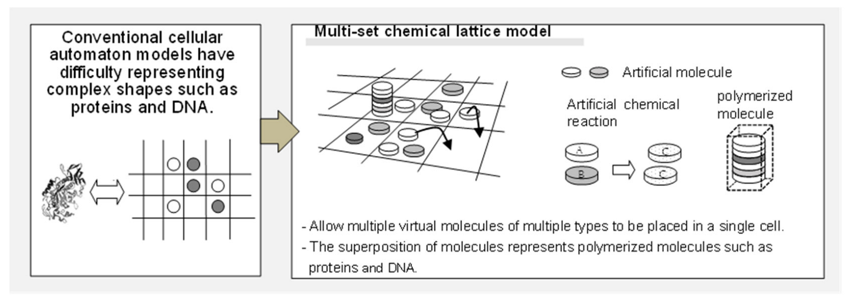
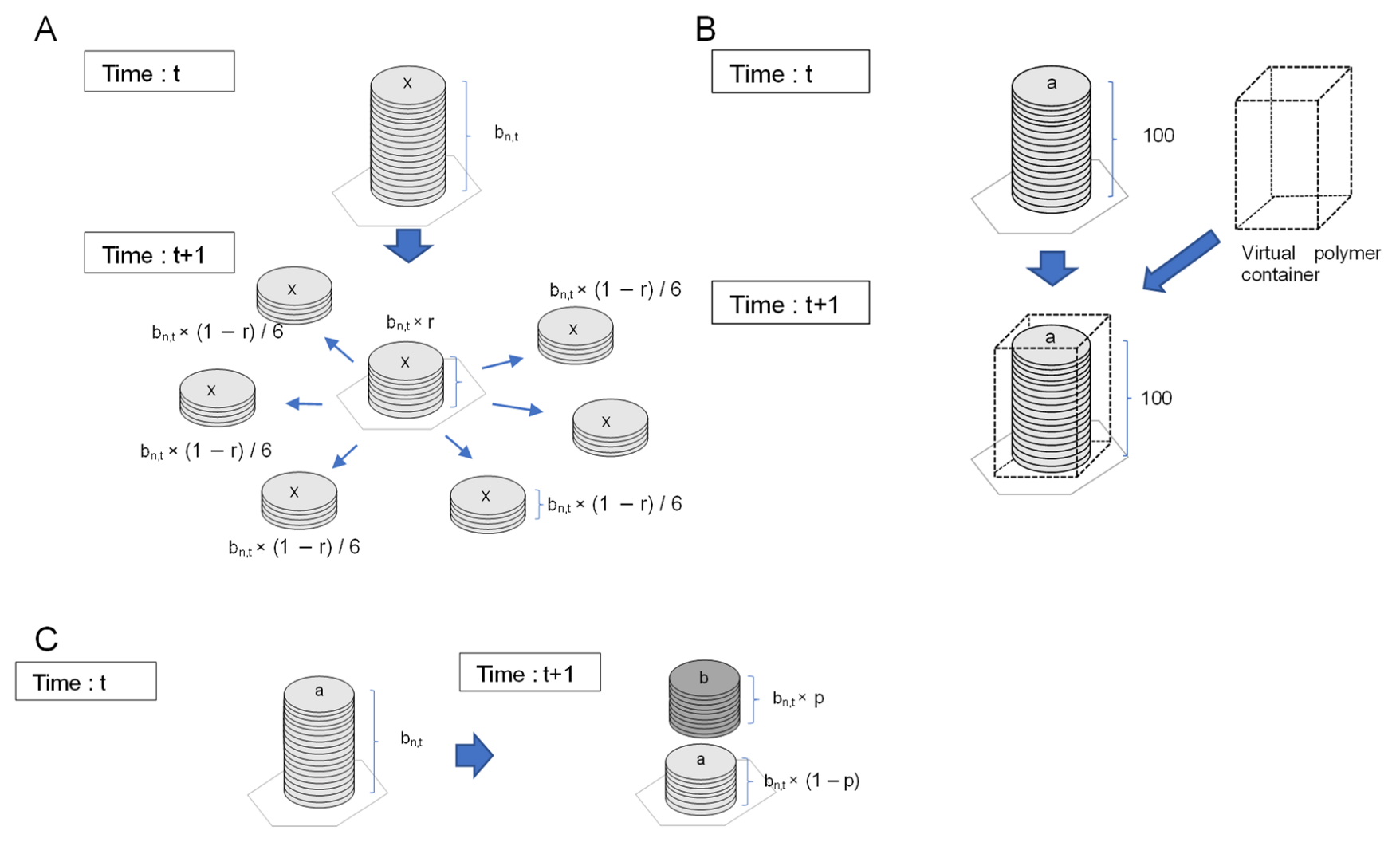
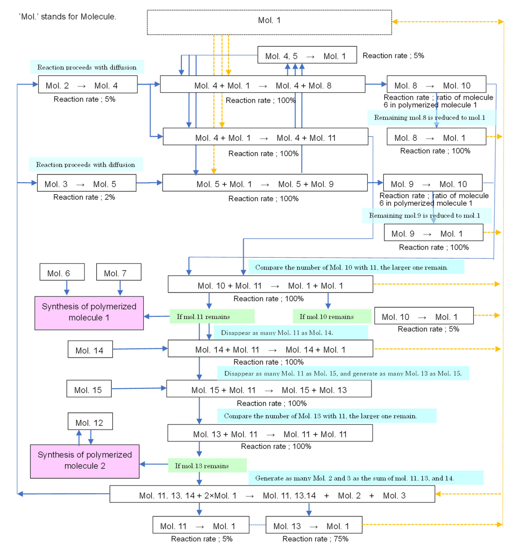
2.1. Model Configuration
- -
- Molecule 1: the material to be converted into each molecule (initially, a large number of such molecules are placed in the lattice space).
- -
- Molecules 2 and 3: correspond to diffusing substances in the Turing pattern model (the difference of diffusion coefficients is expressed by the difference in their residual rate).
- -
- Molecules 4 and 5: substances that change from molecules 2 and 3 during diffusion, respectively.
- -
- Molecules 6 and 7: materials that constitute “polymerized molecule 1,” which is a polymer of molecules 6 and 7 (the ratio of molecules 6 and 7 represents the morphology parameter w).
- -
- Molecules 8, 9, 10, and 11: describe the transition equation of the Ishida model [37] (Equation (1), described below) in chemical reactions.
- -
- Molecule 12: the material that makes up “polymerized molecule 2,” which represents the boundary of the cell.
- -
- Molecules 13, 14, and 15: describe the transition equation of the Ishida model [37] (Equation (2), described below) in chemical reactions.
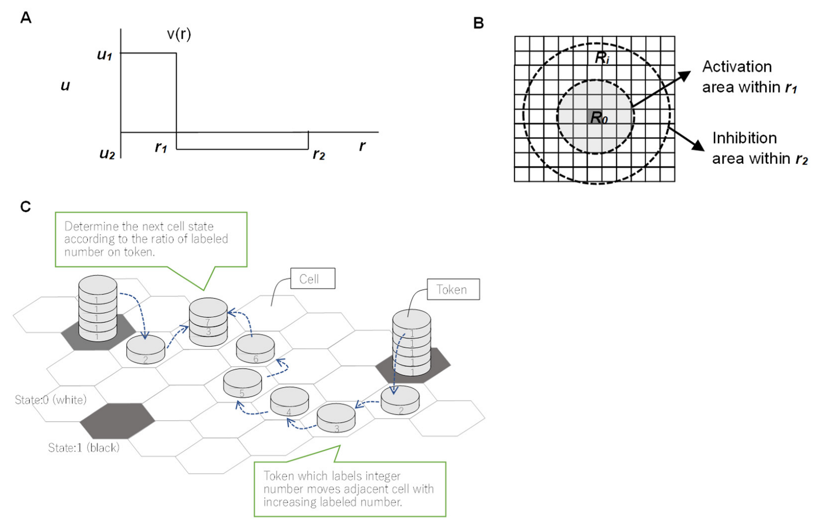
2.2. Conditions for Chemical Reactions to Guide Cellular Emergence
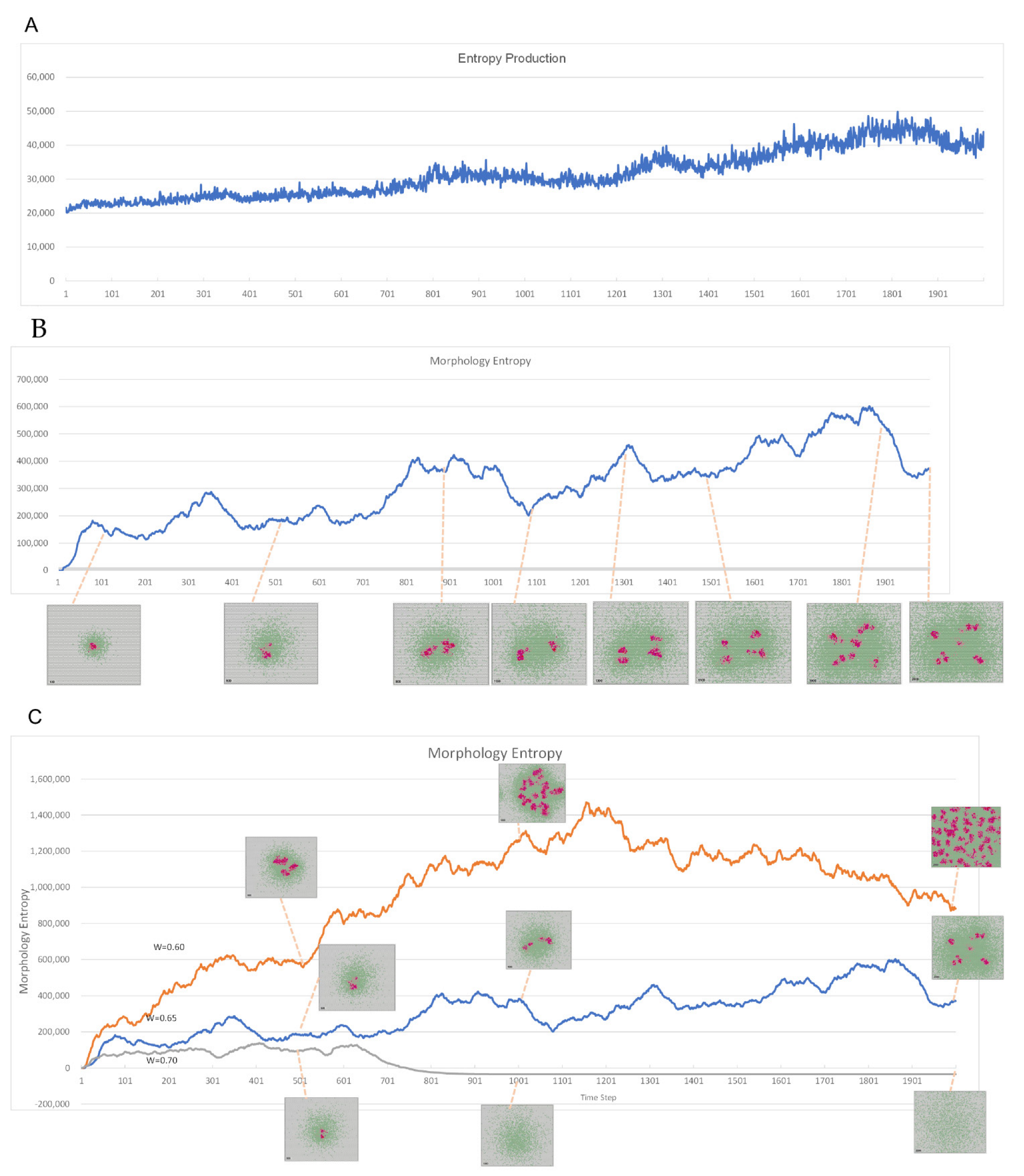
2.3. Method of Evaluation by Entropy
2.3.1. Evaluation Equation for Morphological Entropy
2.3.2. Evaluation Formula for Entropy Production
2.4. Model Implementation
2.4.1. Configuration of Lattice Cell Grids
- -
- Calculation field: 100 × 100 cells in hexagonal grids
- -
- Periodic boundary condition
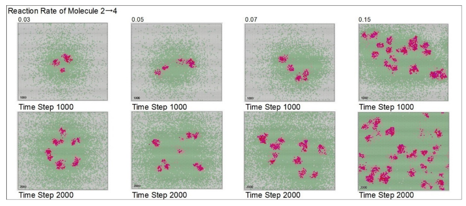
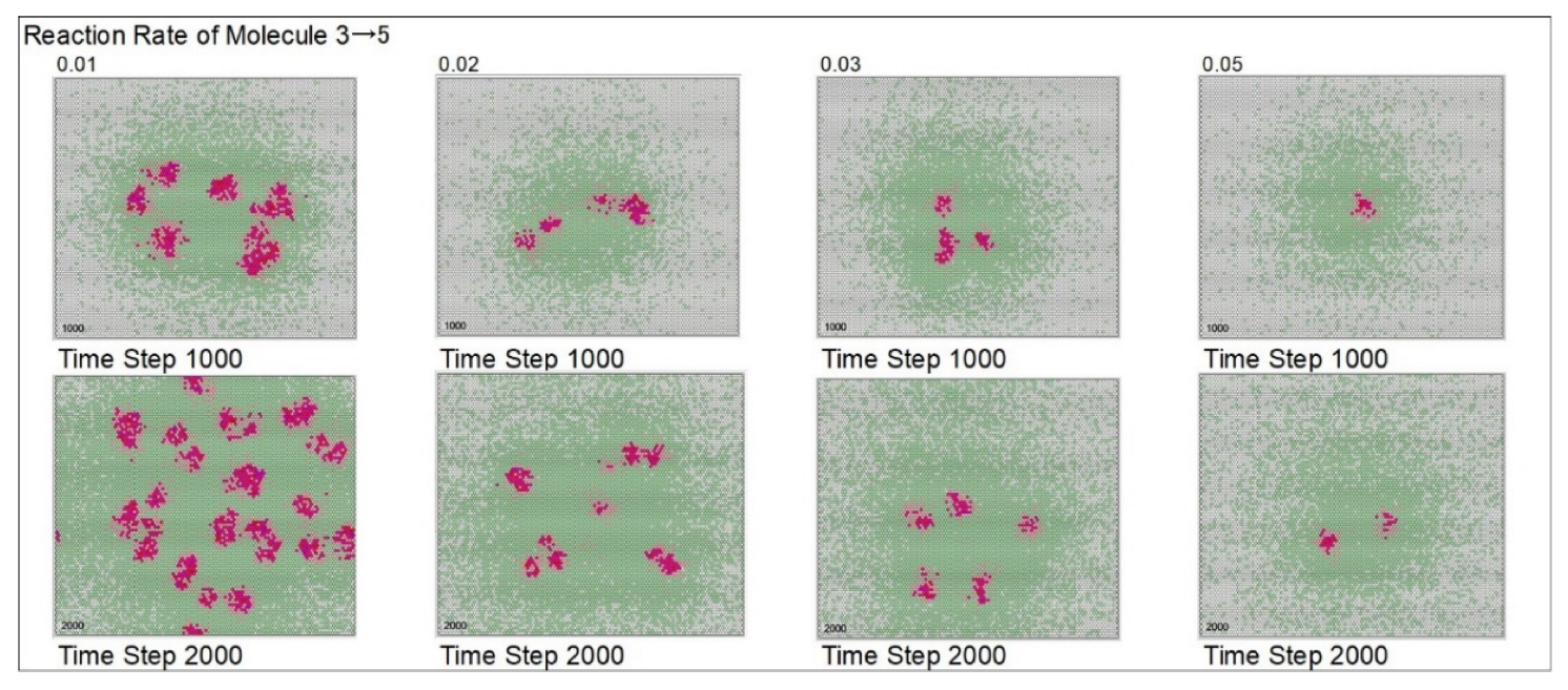
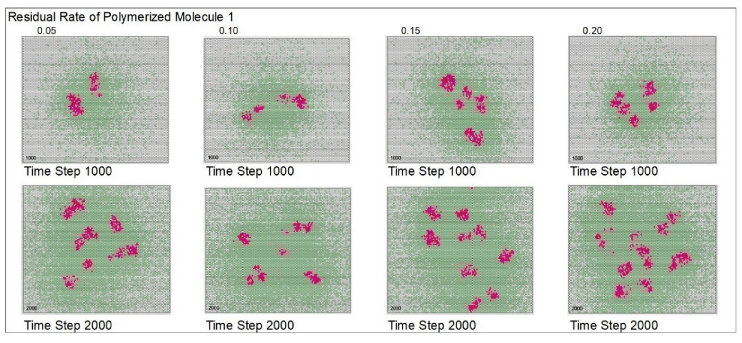
2.4.2. Conditions of Calculations
2.4.3. Initial Conditions
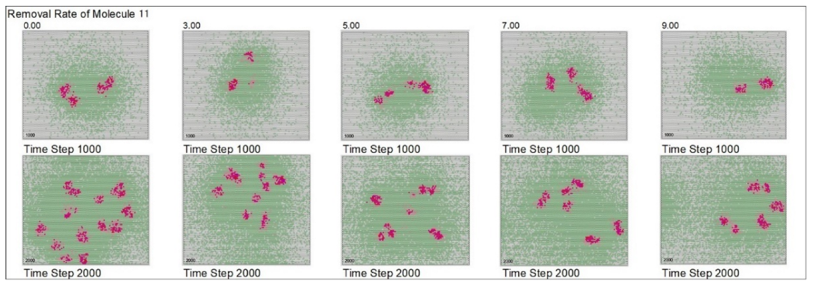
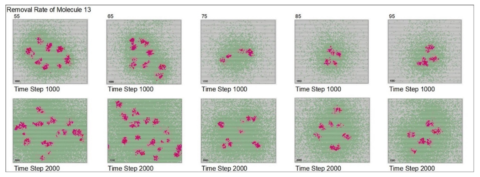
3. Results
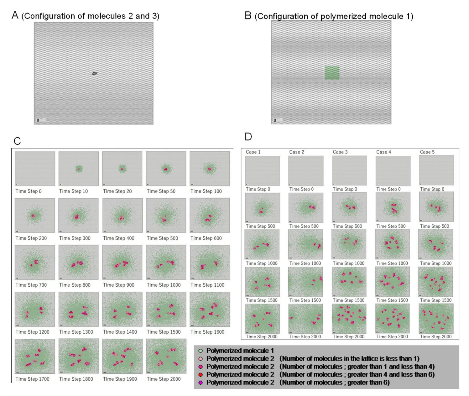
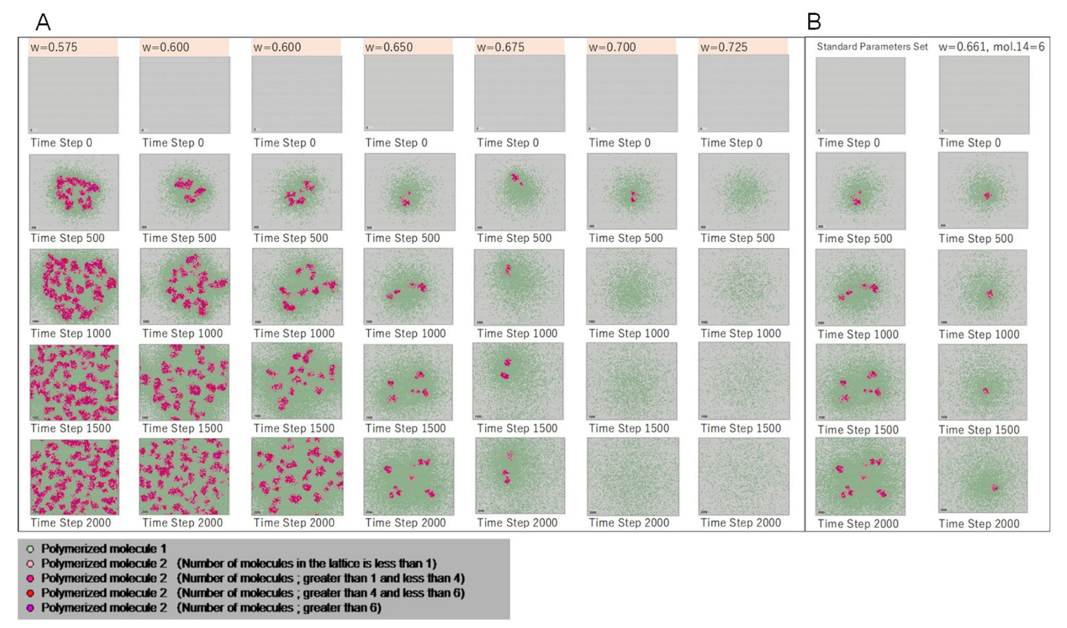
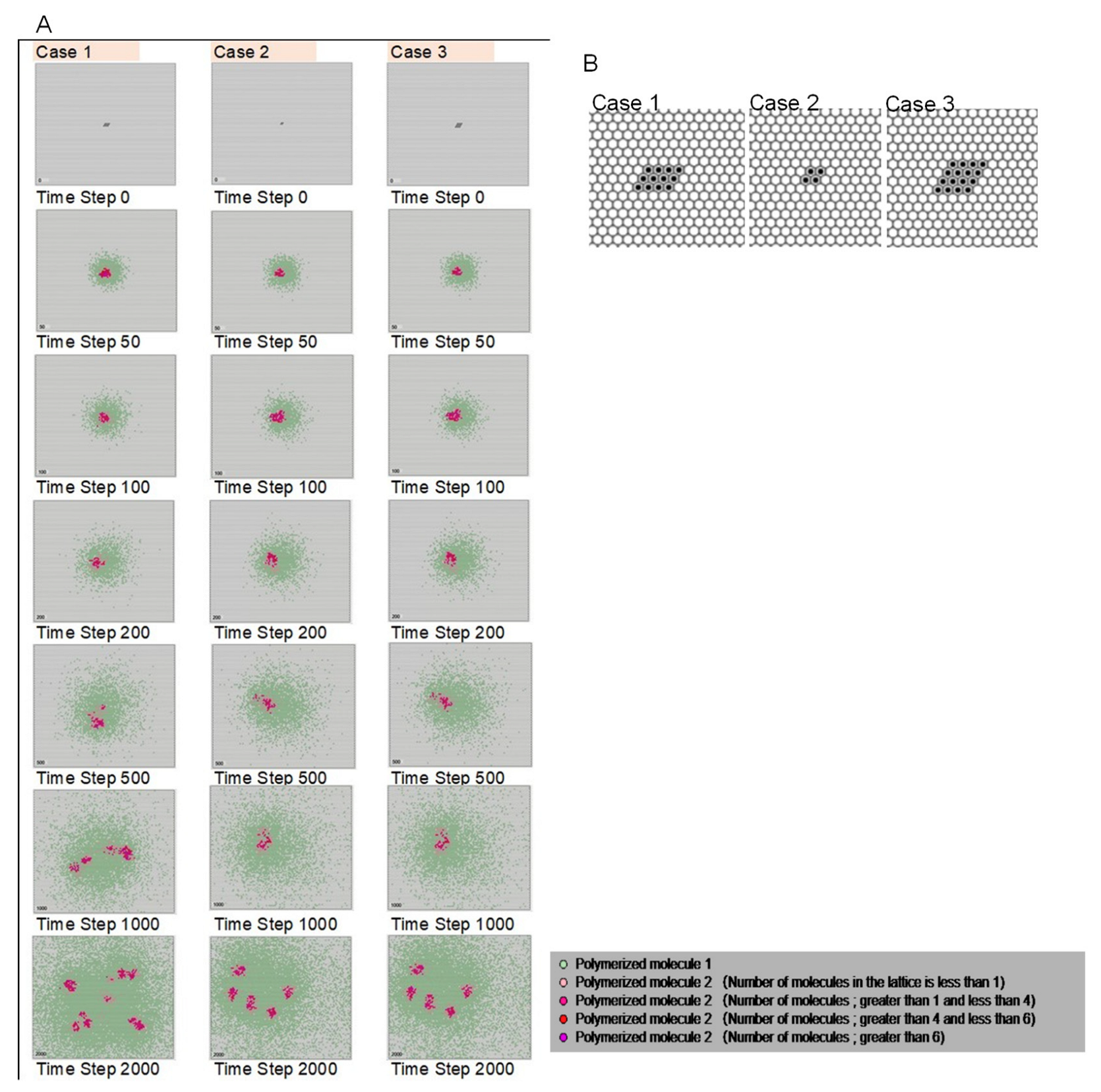
3.1. Emergence of Cell-like Shapes and Their Replication Patterns
- -
- Polymerized molecule 1: molecules 6 and 7 polymerized in the ratio of morphology the parameter w, which controls the shape of the Turing pattern (spots, stripes, etc.) that appears in Equation (1) in the Materials and Methods section. Embedding this information in the lattice space using polymerized molecules was possible. Then, the replication of polymerized molecule 1 represents the propagation of genetic information.
- -
- Polymerized molecule 2: polymerized molecule 2 forms the cell shape (equivalent to membrane molecules).
3.2. Evaluation by Entropy
4. Discussion
- -
- The information that determines the morphology is expressed in terms of the composition ratio of polymerized molecules.
- -
- The model takes into account the replication of polymerized molecules.
5. Conclusions
Supplementary Materials
Funding
Institutional Review Board Statement
Informed Consent Statement
Conflicts of Interest
Appendix A


References
- Gargaud, M.; Martin, H.; Sun, Y. Early Earth and the Origins of Life; Springer: Berlin, Germany, 2013. [Google Scholar]
- Deamer, D. First Life. Discovering the Connections Between Stars, Cells, and How Life Began; University of California Press: Berkeley, CA, USA, 2011. [Google Scholar]
- Kompanichenko, V.N. Inversion concept of the origin of life. Orig. Life Evol. Biosph. 2012, 42, 153–178. [Google Scholar] [CrossRef] [PubMed]
- Kompanichenko, V. The rise of a habitable planet: Four required conditions for the origin of life in the Universe. Geosciences 2019, 9, 92. [Google Scholar] [CrossRef] [Green Version]
- Schrödinger, E. What Is Life–the Physical Aspect of the Living Cell; Cambridge University Press: Cambridge, UK, 1944. [Google Scholar]
- Prigogine, I. Time, structure and fluctuations. Science 1978, 201, 777–785. [Google Scholar] [CrossRef] [PubMed] [Green Version]
- Gilbert, W. Origin of life: The RNA world. Nature 1986, 319, 618. [Google Scholar] [CrossRef]
- Paecht-Horowitz, M.; Berger, J.; Katchalsky, A. Prebiotic Synthesis of Polypeptides by Heterogeneous Polycondensation of amino-acid adenylates. Nature 1970, 228, 636–639. [Google Scholar] [CrossRef]
- Ikehara, K. [GADV]-Protein World Hypothesis on the Origin of Life. Orig. Life Evol. Biosph. 2014, 44, 299–302. [Google Scholar] [CrossRef] [Green Version]
- Djokic, T.; Van Kranendonk, M.J.; Campbell, K.A.; Walter, M.R.; Ward, C.R. Earliest Signs of Life on Land Preserved in ca. 3.5 Ga Hot Spring Deposits. Nat. Commun. 2017, 8, 15263. [Google Scholar] [CrossRef] [Green Version]
- Deamer, D.W.; Georgiou, C.D. Hydrothermal conditions and the origin of cellular life. Astrobiology 2015, 15, 1091–1095. [Google Scholar] [CrossRef]
- Maynard Smith, J. The Problems of Biology; Oxford University Press: Oxford, UK, 1986. [Google Scholar]
- Oparin, A.I.; Synge, A. The Origin of Life on Earth; Academic: New York, NY, USA, 1957. [Google Scholar]
- Miller, S.; Orgel, L.E. The Origin of Life on the Earth; Prentice Hall: Hoboken, NJ, USA, 1974. [Google Scholar]
- Luisi, P.L. The Emergence of Life: From Chemical Origins to Synthetic Biology; Cambridge Univ. Pr.: Cambridge, UK, 2010. [Google Scholar]
- Gibson, D.G.; Glass, J.I.; Lartigue, C.; Noskov, V.N.; Chuang, R.-Y.; Algire, M.A.; Benders, G.A.; Montague, M.G.; Ma, L.; Moodie, M.M.; et al. Creation of a bacterial cell controlled by a chemically synthesized genome. Science 2010, 329, 52–56. [Google Scholar] [CrossRef] [Green Version]
- Gözen, I.; Köksal, E.S.; Põldsalu, I.; Xue, L.; Spustova, K.; Pedrueza-Villalmanzo, E.; Ryskulov, R.; Ryskulov, R.; Meng, F.; Jesorka, A. Protocells: Milestones and recent advances. Small 2022, 18, e2106624. [Google Scholar] [CrossRef]
- Arai, N.; Yoshimoto, Y.; Yasuoka, K.; Ebisuzaki, T. Self-assembly behaviours of primitive and modern lipid membrane solutions: A coarse-grained molecular simulation study. Phys. Chem. Chem. Phys. 2016, 18, 19426–19432. [Google Scholar] [CrossRef] [Green Version]
- Klein, A.; Bock, M.; Alt, W. Simple mechanisms of early life–simulation model on the origin of semi-cells. Biosystems 2017, 151, 34–42. [Google Scholar] [CrossRef]
- Urakami, N.; Jimbo, T.; Sakuma, Y.; Imai, M. Molecular mechanism of vesicle division induced by coupling between lipid geometry and membrane curvatures. Soft Matter 2018, 14, 3018–3027. [Google Scholar] [CrossRef]
- Ghosh, R.; Satarifard, V.; Grafmüller, A.; Lipowsky, R. Budding and fission of nanovesicles induced by membrane adsorption of small solutes. ACS Nano 2021, 15, 7237–7248. [Google Scholar] [CrossRef]
- Thornburg, Z.R.; Bianchi, D.M.; Brier, T.A.; Gilbert, B.R.; Earnest, T.M.; Melo, M.C.; Safronova, N.; Sáenz, J.P.; Cook, A.T.; Wise, K.S.; et al. Fundamental behaviors emerge from simulations of a living minimal cell. Cell 2022, 185, 345–360.e28. [Google Scholar] [CrossRef]
- Gardner, M. The fantastic combinations of John Conway’s new solitaire game ‘life’, mathematical games. Sci. Am. 1970, 223, 120–123. [Google Scholar] [CrossRef]
- Ackley, D.H. (Ed.) Digital protocells with dynamic size, position, and topology. In Proceedings of the ALIFE 2018: The 2018 Conference on Artificial Life, Tokyo, Japan, 23–27 July 2018; MIT Press: Cambridge, MA, USA, 2018. [Google Scholar]
- Ishida, T. Simulations of living cell origins using a cellular automata model. Orig. Life Evol. Biosph. 2014, 44, 125–141. [Google Scholar] [CrossRef]
- Dittrich, P.; Ziegler, J.; Banzhaf, W. Artificial chemistries—A review. Artif. Life 2001, 7, 225–275. [Google Scholar] [CrossRef]
- Kruszewski, G.; Mikolov, T. Emergence of self-reproducing metabolisms as recursive algorithms in an artificial chemistry. Artif. Life 2022, 27, 1–23. [Google Scholar] [CrossRef]
- Fellermann, H.; Rasmussen, S.; Ziock, H.J.; Solé, R.V. Life cycle of a minimal protocell—A dissipative particle dynamics study. Artif. Life 2007, 13, 319–345. [Google Scholar] [CrossRef]
- Hutton, T.J. Evolvable self-reproducing cells in a two-dimensional artificial chemistry. Artif. Life 2007, 13, 11–30. [Google Scholar] [CrossRef]
- Schneider, E.; Mangold, M. Modular assembling process of an in-silico protocell. Biosystems 2018, 165, 8–21. [Google Scholar] [CrossRef] [Green Version]
- Kolezhitskiy, Y.; Egbert, M.; Postlethwaite, C. (Eds.) Dynamical systems analysis of a protocell. In Proceedings of the ALIFE 2020: The 2020 Conference on Artificial Life, Online, 13–18 July 2020; MIT Press: Cambridge, MA, USA, 2020. [Google Scholar]
- Turing, A.M. The chemical basis of morphogenesis. Philos. Trans. R. Soc. Lond. B 1952, 237, 37–72. [Google Scholar]
- Young, D.A. A local activator-inhibitor model of vertebrate skin patterns. Math. Biosci. 1984, 72, 51–58. [Google Scholar] [CrossRef]
- Adamatzky, A.; Martínez, G.J.; Mora, J.C.S.T. Phenomenology of reaction-diffusion binary-state cellular automata. Int. J. Bifürcation Chaos 2006, 16, 2985–3005. [Google Scholar] [CrossRef] [Green Version]
- Dormann, S.; Deutsch, A.; Lawniczak, A.T. Fourier analysis of Turing-like pattern formation in cellular Automaton Models, Future Gen. Comp. Syst. 2001, 17, 901–909. [Google Scholar]
- Tsai, L.L.; Hutchison, G.R.; Peacock-López, E. Turing patterns in a self-replicating mechanism with a self-complementary template. J. Chem. Phys. 2000, 113, 2003–2006. [Google Scholar] [CrossRef]
- Ishida, T. Possibility of controlling self-organized patterns with totalistic cellular automata consisting of both rules like game of life and rules producing Turing patterns. Micromachines 2018, 9, 339. [Google Scholar] [CrossRef] [Green Version]
- Ishida, T. Emergence of Turing patterns in a simple cellular automata-like model via exchange of integer values between adjacent cells. Discrete Dyn. Nat. Soc. 2020, 2020, 2308074. [Google Scholar] [CrossRef]
- Lanier, K.A.; Williams, L.D. The origin of life: Models and data. J. Mol. Evol. 2017, 84, 8592. [Google Scholar] [CrossRef] [Green Version]
- Markus, M.; Hess, B. Isotropic cellular automaton for modeling excitable media. Nature 1990, 347, 56–58. [Google Scholar] [CrossRef]
- Banani, S.F.; Lee, H.O.; Hyman, A.A.; Rosen, M.K. Biomolecular condensates: Organizers of cellular biochemistry. Nat. Rev. Mol. Cell Biol. 2017, 18, 285–298. [Google Scholar] [CrossRef] [PubMed]
- Baum, D.A. Selection and the origin of cells. Bioscience 2015, 65, 678–684. [Google Scholar] [CrossRef] [Green Version]
- Szathmáry, E. Toward major evolutionary transitions theory 2.0. Proc. Natl. Acad. Sci. USA 2015, 112, 10104–10111. [Google Scholar] [CrossRef] [Green Version]
- Hogg, J.R.; Collins, K. Structured non-coding RNAs and the RNP Renaissance. Curr. Opin. Chem. Biol. 2008, 12, 684–689. [Google Scholar] [CrossRef] [Green Version]
- Francis, B.R. An alternative to the RNA world hypothesis. Trends. Evol. Biol. 2011, 3, e2. [Google Scholar] [CrossRef]
- Carter, C.W. What RNA world? Why a peptide–RNA partnership merits renewed experimental attention. Life 2015, 5, 294–320. [Google Scholar] [CrossRef]
- Müller, F.; Escobar, L.; Xu, F.; Węgrzyn, E.; Nainytė, M.; Amatov, T.; Chan, C.; Pichler, A.; Carell, T. A prebiotically plausible scenario of an RNA–peptide world. Nature 2022, 605, 279–284. [Google Scholar] [CrossRef]
- Caetano-Anollés, D.; Caetano-Anollés, K.; Caetano-Anollés, G. Evolution of macromolecular structure: A ‘double tale’ of biological accretion and diversification. Sci. Prog. 2018, 101, 360–383. [Google Scholar] [CrossRef] [Green Version]
- Lane, N. Vital question. In Why Is Life the Way It Is? Profile Books Ltd.: London, UK, 2016. [Google Scholar]
- Kauffman, S.A. A World Beyond Physics: The Emergence and Evolution of Life; Oxford University Press: Oxford, UK, 2019. [Google Scholar]
- Montévil, M.; Mossio, M. Biological organisation as closure of constraints. J. Theor. Biol. 2015, 372, 179–191. [Google Scholar] [CrossRef]


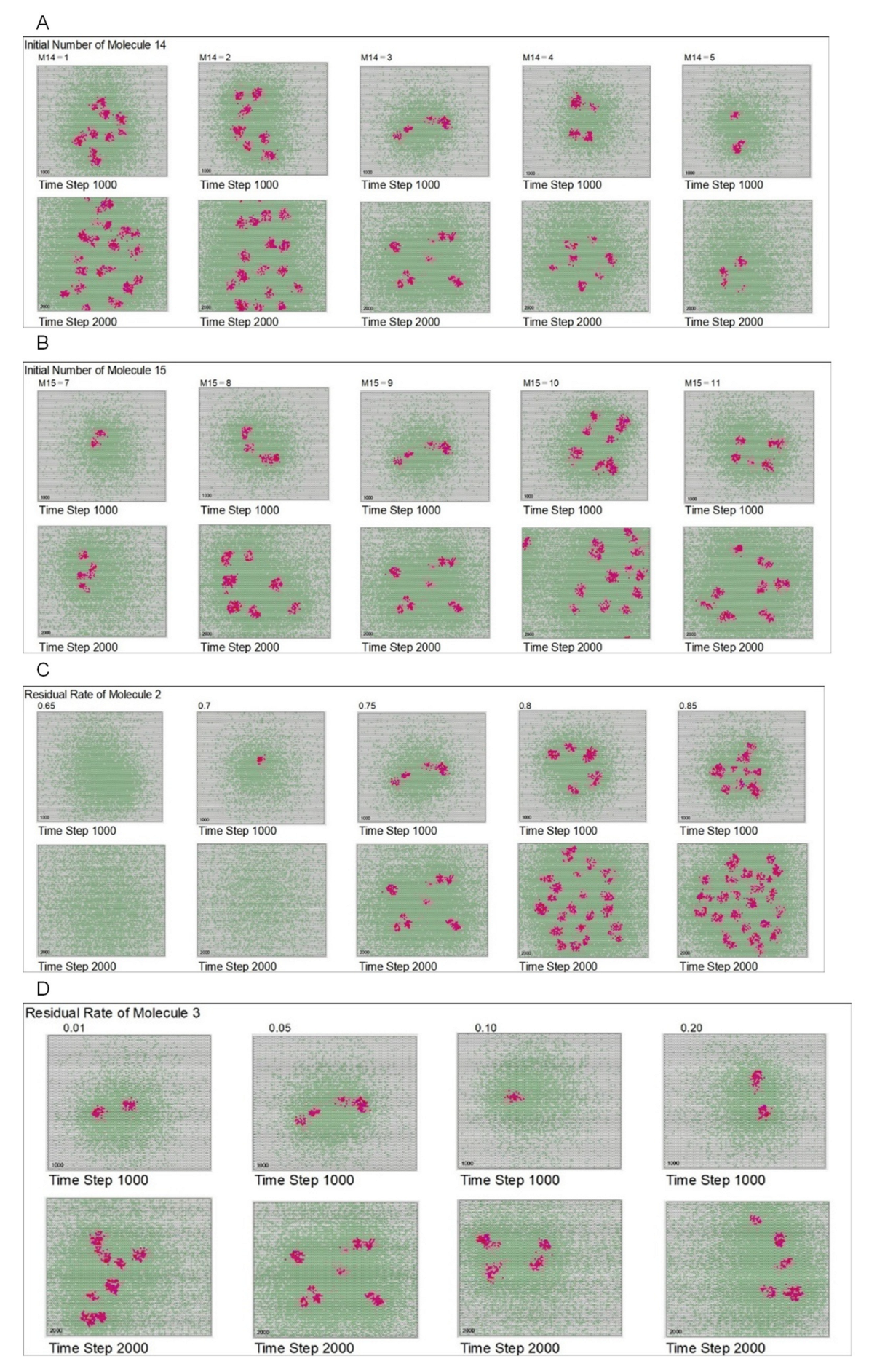
| Focused Parameter | Standard Set of Parameters | Modified Parameters for the Standard Case | ||||||
|---|---|---|---|---|---|---|---|---|
| Parameter w | 0.650 | 0.575 | 0.600 | 0.625 | 0.650 | 0.675 | 0.700 | 0.725 |
| Initial arranged number of mol. 14 | 3 | 1 | 2 | 3 | 4 | 5 | ||
| Initial arranged number of mol. 15 | 9 | 7 | 8 | 9 | 10 | 11 | ||
| Initial configuration of mol.2 and mol. 3 | Case1 | Case1 | Case2 | Case3 | ||||
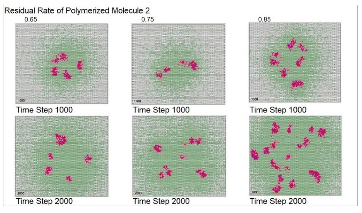
| Residual rate of mol. 2 | 0.75 | 0.65 | 0.70 | 0.75 | 0.80 | 0.85 | ||
| Residual rate of mol. 3 | 0.05 | 0.01 | 0.05 | 0.10 | 0.20 | |||
| Reaction rate of mol. 2 → mol.4 | 5 | 3 | 5 | 7 | 15 | |||
| Reaction rate of mol. 3 → mol.5 | 2 | 1 | 2 | 3 | 5 | |||
| Residual rate of polymerized molecule 1 | 0.1 | 0.05 | 0.1 | 0.15 | 0.2 | |||
| Residual rate of polymerized molecule 2 | 0.75 | 0.65 | 0.75 | 0.85 | ||||
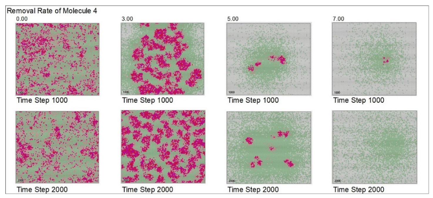
| Removal rate of mol. 4 | 5 | 0 | 3 | 5 | 7 | |||
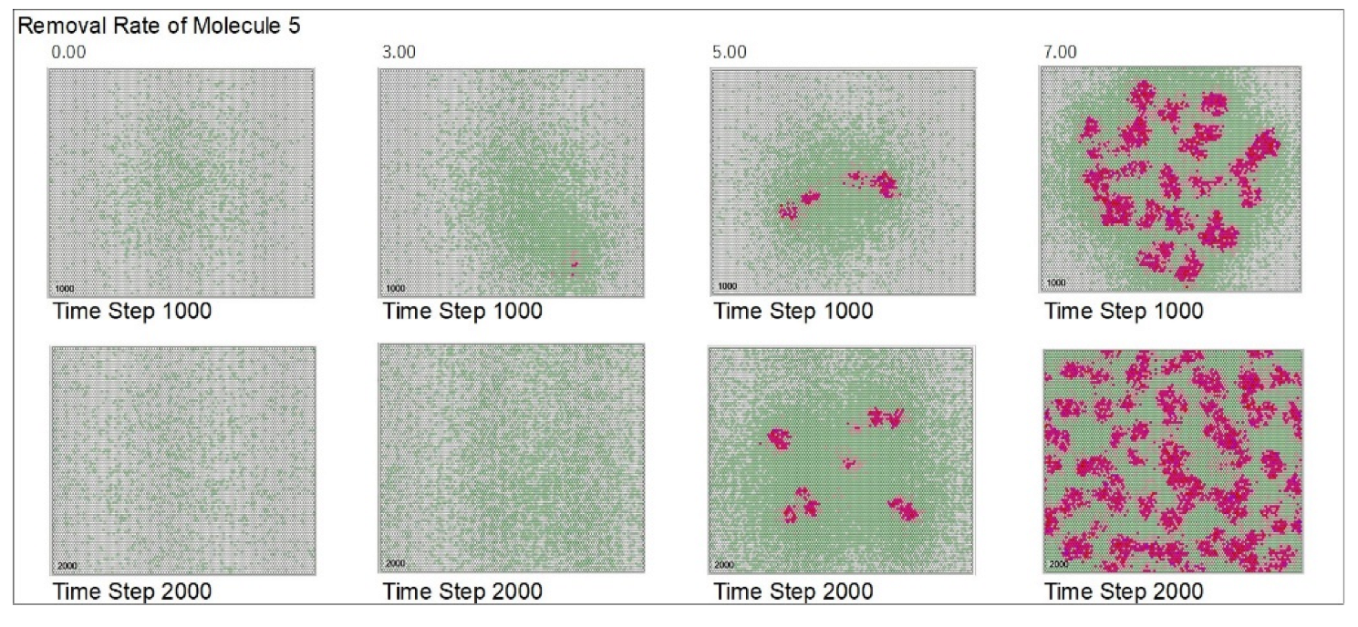
| Removal rate of mol. 5 | 5 | 0 | 3 | 5 | 7 | |||
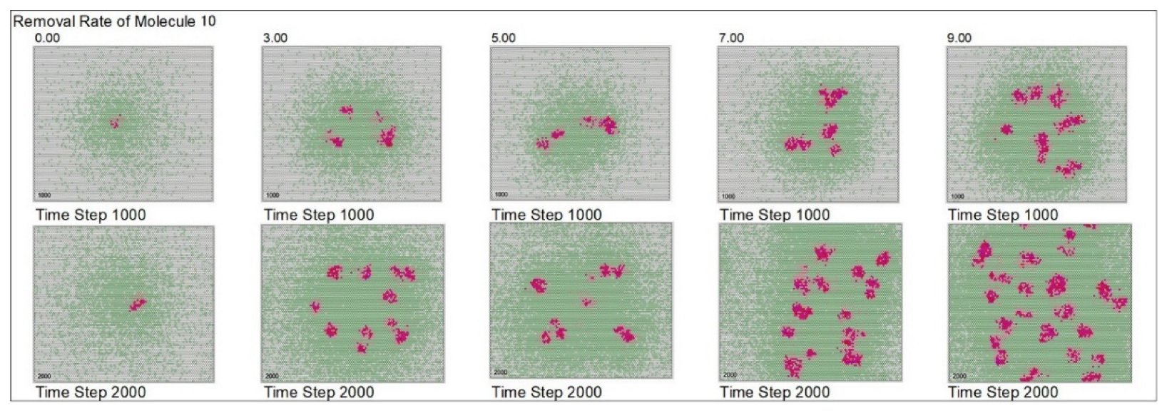
| Removal rate of mol. 10 | 5 | 0 | 3 | 5 | 7 | 9 | ||
| Removal rate of mol. 11 | 5 | 0 | 3 | 5 | 7 | 9 | ||
| Removal rate of mol. 13 | 75 | 55 | 65 | 75 | 80 | 95 | ||
Publisher’s Note: MDPI stays neutral with regard to jurisdictional claims in published maps and institutional affiliations. |
© 2022 by the author. Licensee MDPI, Basel, Switzerland. This article is an open access article distributed under the terms and conditions of the Creative Commons Attribution (CC BY) license (https://creativecommons.org/licenses/by/4.0/).
Share and Cite
Ishida, T. Emergence Simulation of Biological Cell-like Shapes Satisfying the Conditions of Life Using a Lattice-Type Multiset Chemical Model. Life 2022, 12, 1580. https://doi.org/10.3390/life12101580
Ishida T. Emergence Simulation of Biological Cell-like Shapes Satisfying the Conditions of Life Using a Lattice-Type Multiset Chemical Model. Life. 2022; 12(10):1580. https://doi.org/10.3390/life12101580
Chicago/Turabian StyleIshida, Takeshi. 2022. "Emergence Simulation of Biological Cell-like Shapes Satisfying the Conditions of Life Using a Lattice-Type Multiset Chemical Model" Life 12, no. 10: 1580. https://doi.org/10.3390/life12101580