
2D CNN-Based Multi-Output Diagnosis for Compound Bearing Faults under Variable Rotational Speeds


Abstract
:1. Introduction
2. Related Works
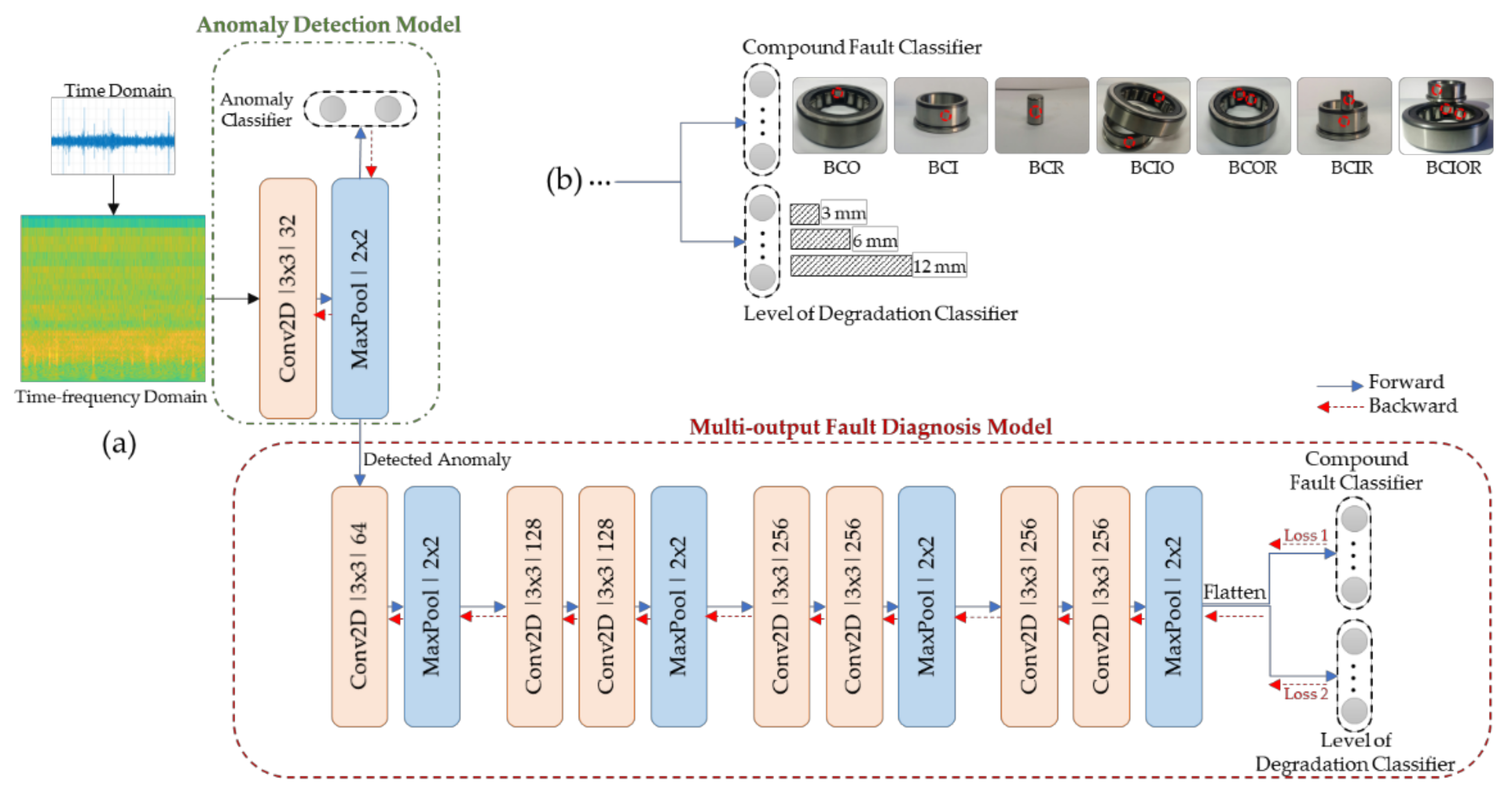
3. Proposed Method
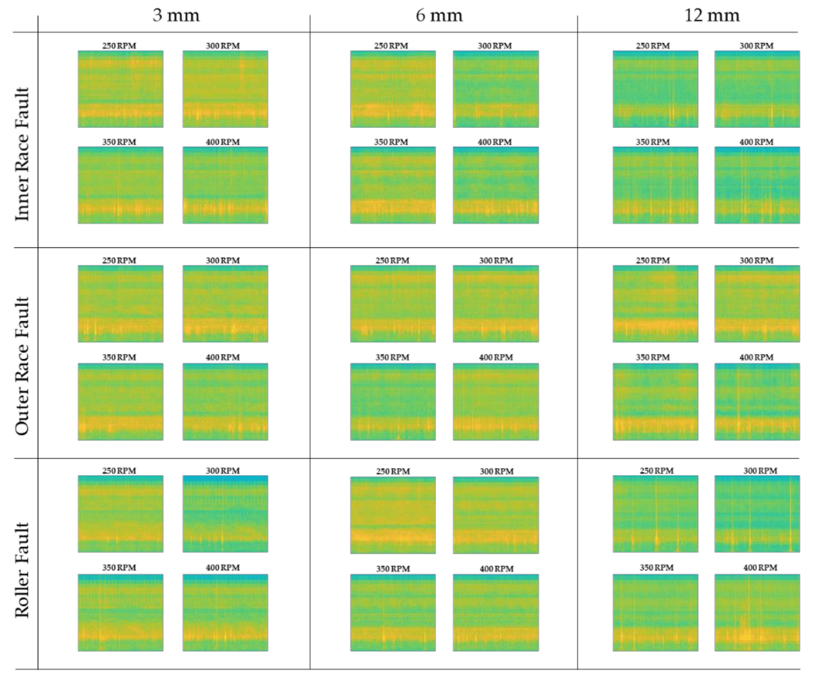
3.1. Time–Frequency Analysis for AE Signals
3.2. Anomaly Detection
3.3. Multi-Output Classification for Compound FD with Degradation Levels
3.3.1. Feature Extraction
3.3.2. Multi-Output Classification
4. Experiments and Results
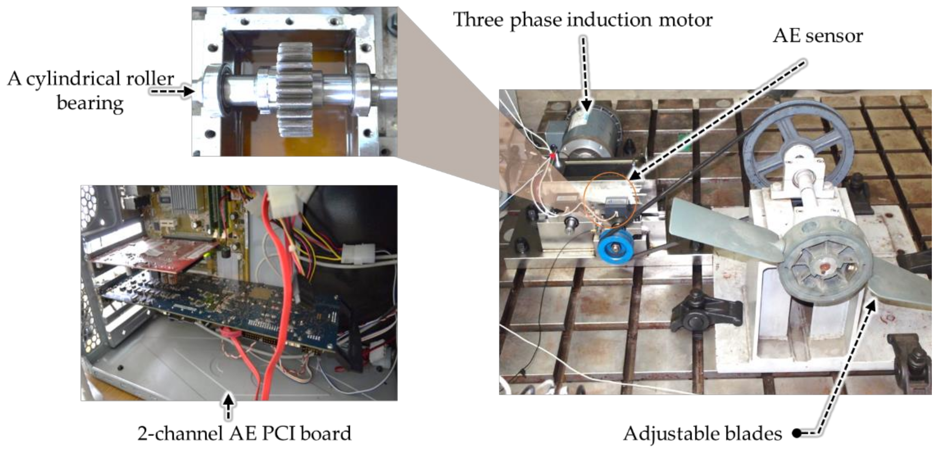
4.1. Experimental System and Dataset
4.2. Evaluation Metrics
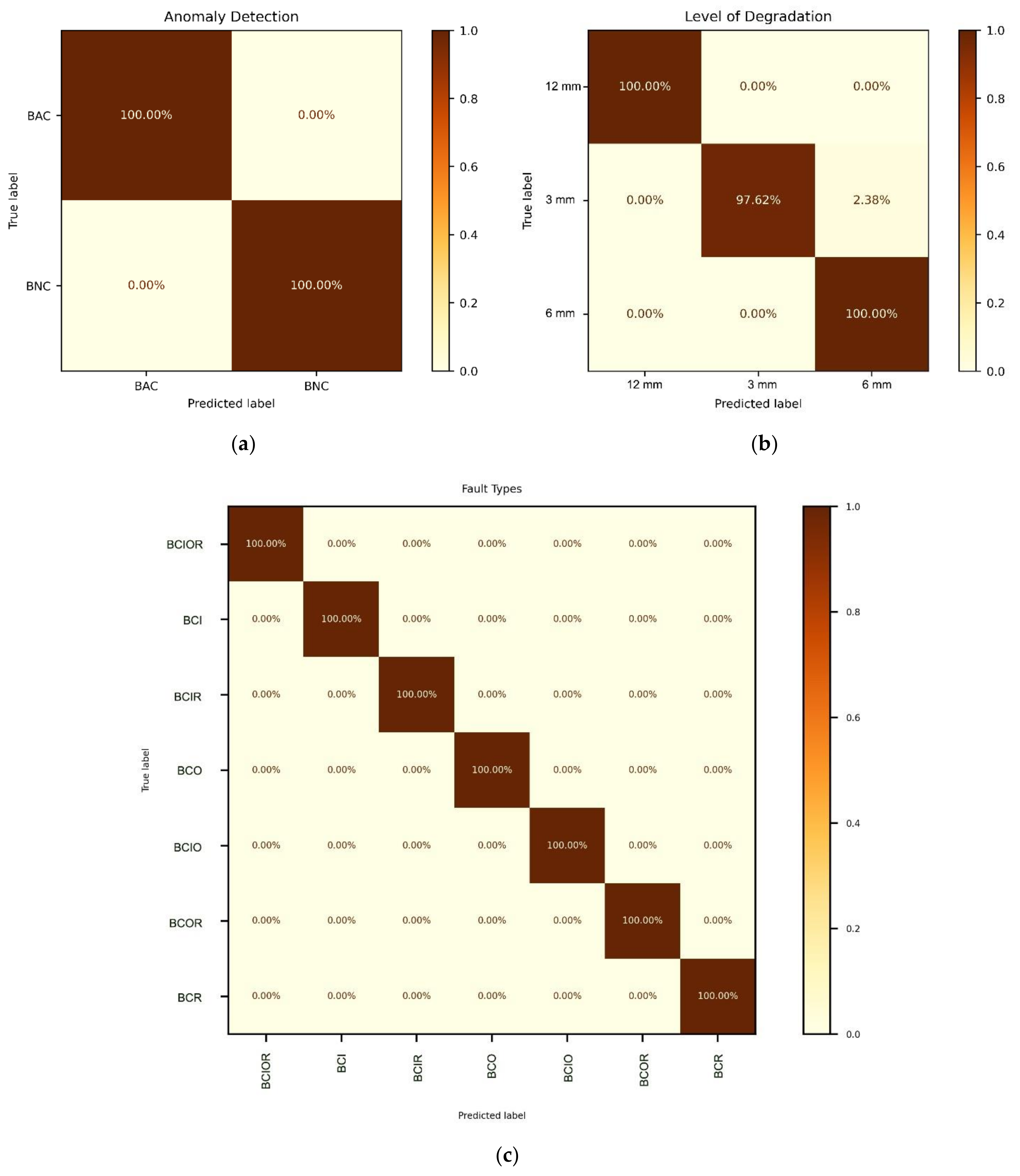
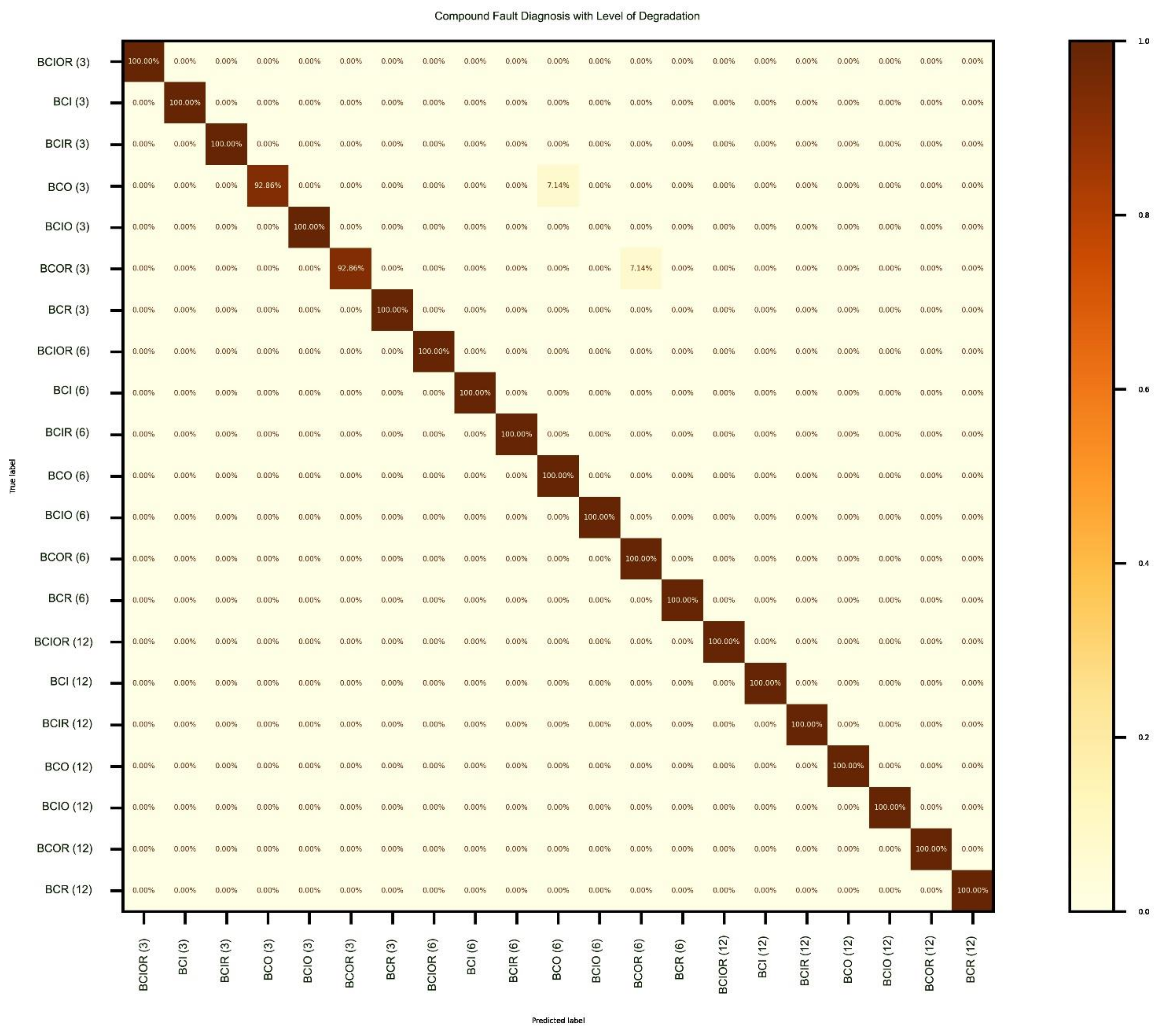
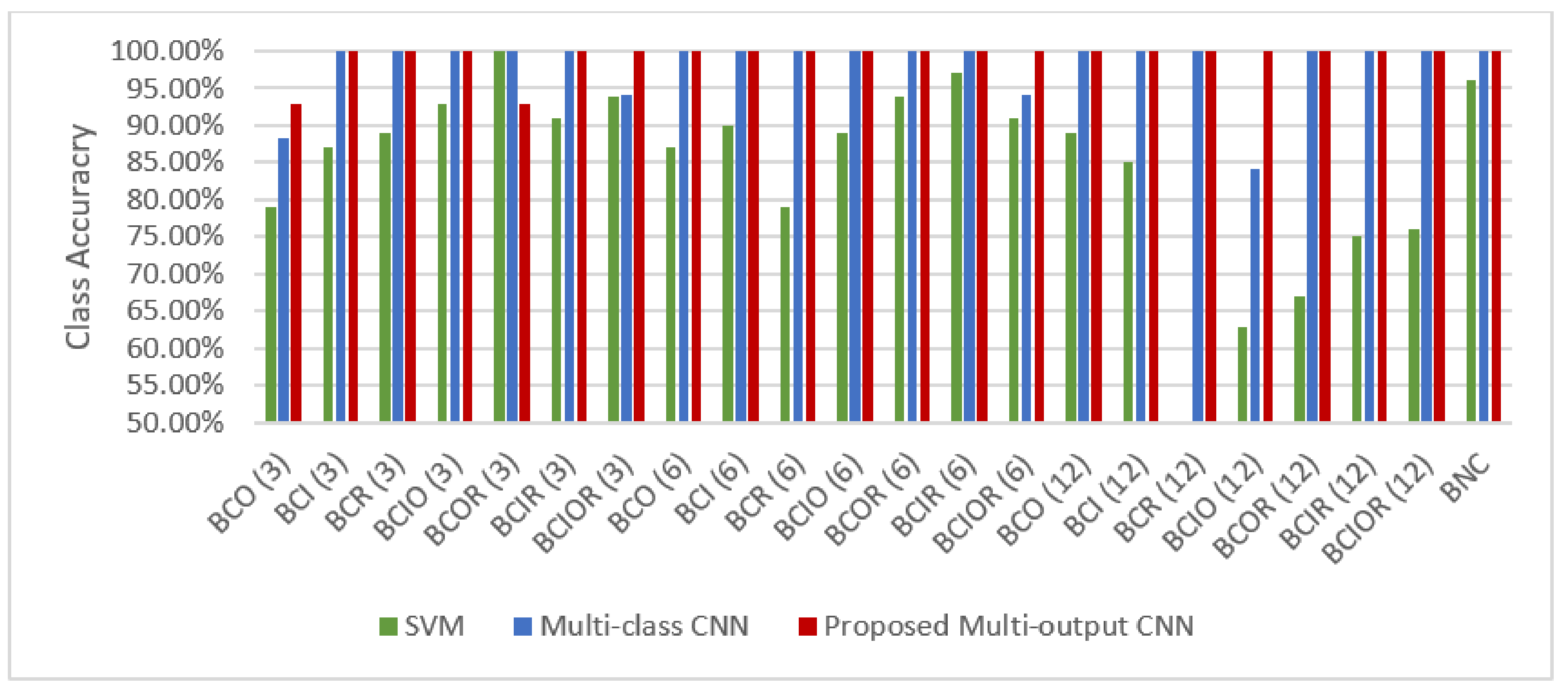
4.3. Classification Results by Using Proposed Multi-Output Classification
4.4. Stability in Noisy Working Environments
5. Conclusions
Author Contributions
Funding
Institutional Review Board Statement
Informed Consent Statement
Data Availability Statement
Conflicts of Interest
References
- O’Donnell, P. Report of Large Motor Reliability Survey of Industrial and Commercial Installations, Part I. IEEE Trans. Ind. Appl. 1985, IA-21, 853–864. [Google Scholar] [CrossRef]
- Bellini, A.; Immovilli, F.; Rubini, R.; Tassoni, C. Diagnosis of Bearing Faults of Induction Machines by Vibration or Current Signals: A Critical Comparison. In Proceedings of the 2008 IEEE Industry Applications Society Annual Meeting, Edmonton, AB, Canada, 5–9 October 2008; pp. 1–8. [Google Scholar]
- Harmouche, J.; Delpha, C.; Diallo, D. Improved Fault Diagnosis of Ball Bearings Based on the Global Spectrum of Vibration Signals. IEEE Trans. Energy Convers. 2015, 30, 376–383. [Google Scholar] [CrossRef]
- Pham, M.T.; Kim, J.-M.; Kim, C.H. Accurate Bearing Fault Diagnosis under Variable Shaft Speed using Convolutional Neural Networks and Vibration Spectrogram. Appl. Sci. 2020, 10, 6385. [Google Scholar] [CrossRef]
- Zhao, B.; Yuan, Q.; Zhang, H. An Improved Scheme for Vibration-Based Rolling Bearing Fault Diagnosis Using Feature Integration and AdaBoost Tree-Based Ensemble Classifier. Appl. Sci. 2020, 10, 1802. [Google Scholar] [CrossRef] [Green Version]
- Schoen, R.; Habetler, T.G.; Kamran, F.; Bartfield, R. Motor bearing damage detection using stator current monitoring. IEEE Trans. Ind. Appl. 1995, 31, 1274–1279. [Google Scholar] [CrossRef]
- Blodt, M.; Granjon, P.; Raison, B.; Rostaing, G. Models for Bearing Damage Detection in Induction Motors Using Stator Current Monitoring. IEEE Trans. Ind. Electron. 2008, 55, 1813–1822. [Google Scholar] [CrossRef] [Green Version]
- Lopez-Perez, D.; Antonino-Daviu, J.A. Application of Infrared Thermography to Failure Detection in Industrial Induction Motors: Case Stories. IEEE Trans. Ind. Appl. 2017, 53, 1901–1908. [Google Scholar] [CrossRef]
- Minervini, M.; Mognaschi, M.E.; Di Barba, P.; Frosini, L. Convolutional Neural Networks for Automated Rolling Bearing Diagnostics in Induction Motors Based on Electromagnetic Signals. Appl. Sci. 2021, 11, 7878. [Google Scholar] [CrossRef]
- Pham, M.T.; Kim, J.-M.; Kim, C.H. Intelligent Fault Diagnosis Method Using Acoustic Emission Signals for Bearings under Complex Working Conditions. Appl. Sci. 2020, 10, 7068. [Google Scholar] [CrossRef]
- Moustafa, W.; Cousinard, O.; Bolaers, F.; Sghir, K.; Dron, J. Low speed bearings fault detection and size estimation using instantaneous angular speed. J. Vib. Control. 2016, 22, 3413–3425. [Google Scholar] [CrossRef]
- Islam, M.M.; Kim, J.-M. Automated bearing fault diagnosis scheme using 2D representation of wavelet packet transform and deep convolutional neural network. Comput. Ind. 2019, 106, 142–153. [Google Scholar] [CrossRef]
- Kim, J.; Kim, J.-M. Bearing Fault Diagnosis Using Grad-CAM and Acoustic Emission Signals. Appl. Sci. 2020, 10, 2050. [Google Scholar] [CrossRef] [Green Version]
- Liu, R.; Yang, B.; Zio, E.; Chen, X. Artificial intelligence for fault diagnosis of rotating machinery: A review. Mech. Syst. Signal Process. 2018, 108, 33–47. [Google Scholar] [CrossRef]
- Zhang, S.; Zhang, S.; Wang, B.; Habetler, T.G. Deep Learning Algorithms for Bearing Fault Diagnostics—A Comprehensive Review. IEEE Access 2020, 8, 29857–29881. [Google Scholar] [CrossRef]
- Khan, S.; Yairi, T. A review on the application of deep learning in system health management. Mech. Syst. Signal Process. 2018, 107, 241–265. [Google Scholar] [CrossRef]
- Cerrada, M.; Sánchez, R.-V.; Li, C.; Pacheco, F.; Cabrera, D.; de Oliveira, J.V.; Vasquez, R.E. A review on data-driven fault severity assessment in rolling bearings. Mech. Syst. Signal Process. 2018, 99, 169–196. [Google Scholar] [CrossRef]
- Liu, S.; Xie, J.; Shen, C.; Shang, X.; Wang, D.; Zhu, Z. Bearing Fault Diagnosis Based on Improved Convolutional Deep Belief Network. Appl. Sci. 2020, 10, 6359. [Google Scholar] [CrossRef]
- Zhang, Y.; Xing, K.; Bai, R.; Sun, D.; Meng, Z. An enhanced convolutional neural network for bearing fault diagnosis based on time–frequency image. Measurement 2020, 157, 107667. [Google Scholar] [CrossRef]
- Tra, V.; Kim, J.; Kim, J.-M. Fault diagnosis of bearings with variable rotational speeds using convolutional neural networks. In Advances in Intelligent Systems and Computing; Springer: Singapore, 2019; pp. 71–81. [Google Scholar] [CrossRef]
- Pham, M.T.; Kim, J.-M.; Kim, C.H. Efficient Fault Diagnosis of Rolling Bearings Using Neural Network Architecture Search and Sharing Weights. IEEE Access 2021, 9, 98800–98811. [Google Scholar] [CrossRef]
- Pham, M.T.; Kim, J.-M.; Kim, C.H. Deep Learning-Based Bearing Fault Diagnosis Method for Embedded Systems. Sensors 2020, 20, 6886. [Google Scholar] [CrossRef]
- Shen, J.; Li, S.; Jia, F.; Zuo, H.; Ma, J. A Deep Multi-Label Learning Framework for the Intelligent Fault Diagnosis of Machines. IEEE Access 2020, 8, 113557–113566. [Google Scholar] [CrossRef]
- Jia, F.; Lei, Y.; Shan, H.; Lin, J. Early Fault Diagnosis of Bearings Using an Improved Spectral Kurtosis by Maximum Correlated Kurtosis Deconvolution. Sensors 2015, 15, 29363–29377. [Google Scholar] [CrossRef] [PubMed]
- Randall, R.; Antoni, J. Rolling element bearing diagnostics—A tutorial. Mech. Syst. Signal Process. 2011, 25, 485–520. [Google Scholar] [CrossRef]
- Zhong, D.; Guo, W.; He, D. An Intelligent Fault Diagnosis Method based on STFT and Convolutional Neural Network for Bearings under Variable Working Conditions. In Proceedings of the 2019 Prognostics and System Health Management Conference (PHM-Qingdao), Qingdao, China, 25–27 October 2019; pp. 1–6. [Google Scholar] [CrossRef]
- Yuan, L.; Lian, D.; Kang, X.; Chen, Y.; Zhai, K. Rolling Bearing Fault Diagnosis Based on Convolutional Neural Network and Support Vector Machine. IEEE Access 2020, 8, 137395–137406. [Google Scholar] [CrossRef]
- Imandoust, S.B.; Bolandraftar, M. Application of K-nearest neighbor (KNN) approach for predicting economic events theoretical background. Int. J. Eng. Res. Appl. 2013, 3, 605–610. [Google Scholar]
- Chen, X.; Wang, S.; Qiao, B.; Chen, Q. Basic research on machinery fault diagnostics: Past, present, and future trends. Front. Mech. Eng. 2018, 13, 264–291. [Google Scholar] [CrossRef] [Green Version]
- Pandya, D.; Upadhyay, S.H.; Harsha, S. Fault diagnosis of rolling element bearing with intrinsic mode function of acoustic emission data using APF-KNN. Expert Syst. Appl. 2013, 40, 4137–4145. [Google Scholar] [CrossRef]
- Baraldi, P.; Cannarile, F.; Di Maio, F.; Zio, E. Hierarchical k-nearest neighbours classification and binary differential evolution for fault diagnostics of automotive bearings operating under variable conditions. Eng. Appl. Artif. Intell. 2016, 56, 1–13. [Google Scholar] [CrossRef] [Green Version]
- Sadegh, H.; Mehdi, A.N.; Mehdi, A. Classification of acoustic emission signals generated from journal bearing at different lubrication conditions based on wavelet analysis in combination with artificial neural network and genetic algorithm. Tribol. Int. 2016, 95, 426–434. [Google Scholar] [CrossRef]
- Yu, Y.; Dejie, Y.; Junsheng, C. A roller bearing fault diagnosis method based on EMD energy entropy and ANN. J. Sound Vib. 2006, 294, 269–277. [Google Scholar] [CrossRef]
- Ben Ali, J.; Fnaiech, N.; Saidi, L.; Chebel-Morello, B.; Fnaiech, F. Application of empirical mode decomposition and artificial neural network for automatic bearing fault diagnosis based on vibration signals. Appl. Acoust. 2015, 89, 16–27. [Google Scholar] [CrossRef]
- Rafi, M.; Shaikh, M.S. A comparison of SVM and RVM for Document Classification 2013. Available online: http://arxiv.org/abs/1301.2785 (accessed on 15 August 2021).
- Jiang, L.-L.; Yin, H.-K.; Li, X.-J.; Tang, S.-W. Fault Diagnosis of Rotating Machinery Based on Multisensor Information Fusion Using SVM and Time-Domain Features. Shock. Vib. 2014, 2014, 418178. [Google Scholar] [CrossRef]
- Hui, K.H.; Lim, M.H.; Leong, M.S.; Al-Obaidi, S.M. Dempster-Shafer evidence theory for multi-bearing faults diagnosis. Eng. Appl. Artif. Intell. 2017, 57, 160–170. [Google Scholar] [CrossRef]
- Bhadane, M.; Ramachandran, K.I. Bearing fault identification and classification with convolutional neural network. In Proceedings of the 2017 International Conference on Circuit, Power and Computing Technologies (ICCPCT), Kollam, India, 20–21 April 2017; pp. 17–21. [Google Scholar]
- Shao, Y.; Yuan, X.; Zhang, C.; Song, Y.; Xu, Q. A Novel Fault Diagnosis Algorithm for Rolling Bearings Based on One-Dimensional Convolutional Neural Network and INPSO-SVM. Appl. Sci. 2020, 10, 4303. [Google Scholar] [CrossRef]
- Zhou, X.; Mao, S.; Li, M. A Novel Anti-Noise Fault Diagnosis Approach for Rolling Bearings Based on Convolutional Neural Network Fusing Frequency Domain Feature Matching Algorithm. Sensors 2021, 21, 5532. [Google Scholar] [CrossRef] [PubMed]
- Ince, T.; Kiranyaz, S.; Eren, L.; Askar, M.; Gabbouj, M. Real-Time Motor Fault Detection by 1-D Convolutional Neural Networks. IEEE Trans. Ind. Electron. 2016, 63, 7067–7075. [Google Scholar] [CrossRef]
- Zan, T.; Wang, H.; Wang, M.; Liu, Z.; Gao, X. Application of Multi-Dimension Input Convolutional Neural Network in Fault Diagnosis of Rolling Bearings. Appl. Sci. 2019, 9, 2690. [Google Scholar] [CrossRef] [Green Version]
- Li, G.; Deng, C.; Wu, J.; Chen, Z.; Xu, X. Rolling Bearing Fault Diagnosis Based on Wavelet Packet Transform and Convolutional Neural Network. Appl. Sci. 2020, 10, 770. [Google Scholar] [CrossRef] [Green Version]
- Zhuang, Z.; Lv, H.; Xu, J.; Qin, W. A Deep Learning Method for Bearing Fault Diagnosis through Stacked Residual Dilated Convolutions. Appl. Sci. 2019, 9, 1823. [Google Scholar] [CrossRef] [Green Version]
- Ma, H.; Li, S.; An, Z. An A Fault Diagnosis Approach for Rolling Bearing Based on Convolutional Neural Network and Nuisance Attribute Projection under Various Speed Conditions. Appl. Sci. 2019, 9, 1603. [Google Scholar] [CrossRef] [Green Version]
- Jeong, H.; Park, S.; Woo, S.; Lee, S. Rotating Machinery Diagnostics Using Deep Learning on Orbit Plot Images. Procedia Manuf. 2016, 5, 1107–1118. [Google Scholar] [CrossRef] [Green Version]
- Han, T.; Liu, C.; Yang, W.; Jiang, D. A novel adversarial learning framework in deep convolutional neural network for intelligent diagnosis of mechanical faults. Knowl. Based Syst. 2019, 165, 474–487. [Google Scholar] [CrossRef]
- Verstraete, D.; Ferrada, A.; Droguett, E.L.; Meruane, V.; Modarres, M. Deep Learning Enabled Fault Diagnosis Using Time-Frequency Image Analysis of Rolling Element Bearings. Shock. Vib. 2017, 2017, 5067651. [Google Scholar] [CrossRef]
- Yuan, Z.; Zhang, L.; Duan, L.; Li, T. Intelligent Fault Diagnosis of Rolling Element Bearings Based on HHT and CNN. In Proceedings of the 2018 Prognostics System Health Management Conference (PHM-Chongqing), Chongqing, China, 26–28 October 2018; pp. 292–296. [Google Scholar] [CrossRef]
- Baxter, J. A Bayesian/Information Theoretic Model of Learning to Learn via Multiple Task Sampling. Mach. Learn. 1997, 28, 7–39. [Google Scholar] [CrossRef]
- Vaswani, S.; Mishkin, A.; Laradji, I.; Schmidt, M.; Gidel, G.; Lacoste-Julien, S. Painless Stochastic Gradient: Interpolation, Line-Search, and Convergence Rates. 2019. Available online: http://arxiv.org/abs/1905.09997 (accessed on 15 August 2021).
- Armijo, L. Minimization of functions having Lipschitz continuous first partial derivatives. Pac. J. Math. 1966, 16, 1–3. [Google Scholar] [CrossRef] [Green Version]


| Contact angle | 0° |
| Number of rolling elements | 13 |
| Pitch diameter | 46.5 (mm) |
| Rolling element diameter | 9.0 (mm) |
| Single and Compound Bearing Defect Dataset | Rotational Speed (rpm) | Crack Size | ||
|---|---|---|---|---|
| Length (mm) | Width (mm) | Depth (mm) | ||
| Training subset | 300, 400, 500 | 3 | 0.6 | 0.3 |
| 6 | 0.6 | 0.5 | ||
| 12 | 0.6 | 0.5 | ||
| Validation subset; Testing subset | 250, 350, 450 | 3 | 0.6 | 0.3 |
| 6 | 0.6 | 0.5 | ||
| 12 | 0.6 | 0.5 | ||
| Abbr. | Fault Category (Fault Type—Crack Size) | Multi-Output Labels | |
|---|---|---|---|
| Fault Type | Crack Size | ||
| BCO (3) | Outer raceway (3 mm) | 1 | 1 |
| BCI (3) | Inner raceway (3 mm) | 2 | 1 |
| BCR (3) | Roller (3 mm) | 3 | 1 |
| BCIO (3) | Inner and outer raceway (3 mm) | 4 | 1 |
| BCOR (3) | Outer raceway and roller (3 mm) | 5 | 1 |
| BCIR (3) | Inner raceway and roller (3 mm) | 6 | 1 |
| BCIOR (3) | Inner, outer raceway, roller (3 mm) | 7 | 1 |
| BCO (6) | Outer raceway (6 mm) | 1 | 2 |
| BCI (6) | Inner raceway (6 mm) | 2 | 2 |
| BCR (6) | Roller (6 mm) | 3 | 2 |
| BCIO (6) | Inner and outer raceway (6 mm) | 4 | 2 |
| BCOR (6) | Outer raceway and roller (6 mm) | 5 | 2 |
| BCIR (6) | Inner raceway and roller (6 mm) | 6 | 2 |
| BCIOR (6) | Inner, outer raceway, roller (6 mm) | 7 | 2 |
| BCO (12) | Outer raceway (12 mm) | 1 | 3 |
| BCI (12) | Inner raceway (12 mm) | 2 | 3 |
| BCR (12) | Roller (12 mm) | 3 | 3 |
| BCIO (12) | Inner and outer raceway (12 mm) | 4 | 3 |
| BCOR (12) | Outer raceway and roller (12 mm) | 5 | 3 |
| BCIR (12) | Inner raceway and roller (12 mm) | 6 | 3 |
| BCIOR (12) | Inner, outer raceway, roller (12 mm) | 7 | 3 |
| BNC | Normal state | ||
| BAC | Abnormal state | ||
| Number of MAC | Number of Parameters | |
|---|---|---|
| Multi-class CNN [10] | 195M | 5.3M |
| Proposed multi-output CNN | 1.9M | 2.31M |
| Proposed ADM | 0.05M | 962 |
| SNR | ACA | |
|---|---|---|
| Multi-Class CNN [10] | Proposed Multi-Output CNN | |
| No noise | 98.21 | 99.32 |
| 10 | 96.08 | 98.65 |
| 5 | 95.36 | 97.82 |
| 0 | 93.33 | 95.87 |
Publisher’s Note: MDPI stays neutral with regard to jurisdictional claims in published maps and institutional affiliations. |
© 2021 by the authors. Licensee MDPI, Basel, Switzerland. This article is an open access article distributed under the terms and conditions of the Creative Commons Attribution (CC BY) license (https://creativecommons.org/licenses/by/4.0/).
Share and Cite
Pham, M.-T.; Kim, J.-M.; Kim, C.-H. 2D CNN-Based Multi-Output Diagnosis for Compound Bearing Faults under Variable Rotational Speeds. Machines 2021, 9, 199. https://doi.org/10.3390/machines9090199
Pham M-T, Kim J-M, Kim C-H. 2D CNN-Based Multi-Output Diagnosis for Compound Bearing Faults under Variable Rotational Speeds. Machines. 2021; 9(9):199. https://doi.org/10.3390/machines9090199
Chicago/Turabian StylePham, Minh-Tuan, Jong-Myon Kim, and Cheol-Hong Kim. 2021. "2D CNN-Based Multi-Output Diagnosis for Compound Bearing Faults under Variable Rotational Speeds" Machines 9, no. 9: 199. https://doi.org/10.3390/machines9090199