Sub-Health Identification of Reciprocating Machinery Based on Sound Feature and OOD Detection

Abstract

It is inevitable that machine parts will be worn down in production, causing other mechanical failures. With the appearance of wearing, the accuracy and efficiency of machinery gradually decline. The state between healthy and impaired is defined as sub-health. By recognizing the sub-health state of machinery, accuracy and efficiency can be effectively guaranteed, and the occurrence of mechanical failure can be prevented. Compared with simple fault detection, the identification of s sub-health state has more practical significance. For this reason, the sound characteristics of large-scale reciprocating machinery, combined with the concept of OOD (out-of-distribution) detection, are used, and a model for detecting machinery sub-health state is proposed. A planer sound dataset was collected and collated, and the recognition of mechanical sub-health state was realized by a model combining a VGG network and the threshold setting scheme of OOD detection. Finally, an auxiliary decision-making module was added, and Mahalanobis distance was used to represent spatial relationships among samples, further improving the recognition effect.

1. Introduction

Machinery is an indispensably essential part of society, and it has been since the industrial revolution. Mechanical sub-health state is a transition state between a normal state and a damage state. The standard of mechanical sub-health is manifested as decreasing accuracy and efficiency, or an increasing defective rate, but it does not meet the criteria for mechanical failure. The sub-health state of machinery is not fixed, and it can be changed according to actual needs; its identification can ensure that a given piece of machinery is working in its best state. There are obvious differences between a fault sound and a normal sound. Thus, in order to identify the sub-health state of machinery, ascertaining whether a machine is faulty or not should be considered first; only then can its sub-health state be established. In recent years, the intelligent fault diagnosis technology of deep learning has becoming increasingly mature, and the efficiency of fault diagnosis has continuously improved. Currently, mainstream methods use vibration sensors to collect one-dimensional vibration signals, which are then converted into two-dimensional signals and used through a neural network to diagnose the state of a given machine [1]. However, heavy machinery has great stability, as well as local vibration that a low impact. Due to this, some main working parts are inconvenient objects on which to install vibration sensors, leading to the recognition effects being imprecise.

More recent fault diagnoses mainly use vibration signal characteristics. For example, W. Zhang et al. [2] used a novel method named deep convolutional neural networks with wide first-layer kernels (WDCNN) for fault diagnosis. Q. Hang et al. [3] used high-dimensional imbalance data to diagnose rolling bearings. W. Sun et al. [4] proposed a motor fault detection method based on a sparse autoencoder. In early research, sound detection technology and sound source localization were initially used in military applications, such as sonar exploration, detection, and localization. With developments in technology, sound detection technology has gradually been applied in various fields. For example, Yiallourides and Naylor [5] used knee joint sound time–frequency analysis for the non-invasive detection of osteoarthritis. Das et al. [6] used acoustic features by unsupervised learning for heart sound event detection. In addition, Bayram [7] used sequence auto-encoders to detect anomalies in industrial processes, while Liu [8] also detected healthy broilers by using abnormal sounds. Tran and Lundgren [9] proposed a drill fault diagnosis method based on an intelligent acoustic signals scale spectrum and the Mel spectrum. Wang et al. [10] used sound signals to detect and locate pipelines leaks. Volkmann et al. [11] and Hou et al. [12] used sound signals to detect the injury on cows’ feet and the longitudinal tears of a conveyor belt, respectively. Further, Ramteke et al. [13] outlined a fault diagnosis method for a diesel engine cylinder liner wear fault based on vibration and acoustic emission analysis. There are more others who have theorized equipment health state condition monitoring and fault detection using acoustic signals. Common mechanical fault diagnosis mainly focuses on rotating machinery intelligent diagnosis, such as bearings and gearboxes, and the majority of these datasets were collected on analog equipment. Due to the fact that such equipment has great lubrication, and because its sound features are not obvious, the results of vibration signals are better than sound signals. However, in large-scale and heavy-duty reciprocating equipment, due to the technical requirements for good stability, the vibration effect of key working parts is not obvious, and the sound is relatively loud. In light of this condition, the use of sound characteristics can achieve more comprehensive results.

Under normal circumstances, if a convolutional neural network is used to identify a mechanical state, a large number of normal and abnormal sound samples are needed. In real work, normal sounds are often smooth and regular, and they are accompanied by an obvious abnormal sound when a machine breaks down; however, it is difficult for us to collect abnormal data without deliberately damaging machinery. In 2018, Dan Hendrycks et al. [14] proposed a novel OOD detection baseline with deep learning based on abnormal detection. The model used positive samples as in-distribution data by training the positive samples, and the in-distribution data and out-of-distribution data could be clearly distinguished; this approach is suitable for actual situations related to mechanical fault detection. Moreover, Liang et al. [15] improved the baseline and proposed an ODIN (Out-of-distribution detector for Neural networks) model, while Devries et al. [16], Shalev et al. [17], Denouden et al. [18], Abdelzad et al. [19], and others improved the baseline in different directions, thus improving detection efficacy.

Based on the above description, we propose the use of deep convolutional neural networks to extract sound features, and we use OOD detection technology to recognize mechanical sub-health state with normal sample data as input. The remaining part of this paper includes four sections: Section 2 introduces the dataset collected and organized by us. Section 3 introduces our experimental method. Section 4 uses three interrelated experiments to prove that using sound features and OOD detection can greatly identify mechanical sub-health state. Finally, a conclusion is drawn in Section 5.

The contributions of this paper can be summarized as follows:

(1)

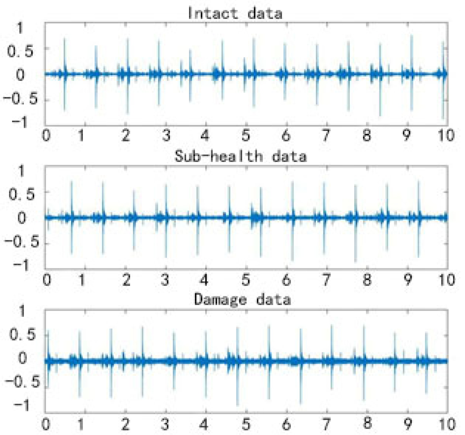
A kind of mechanical running state is defined, which is called a mechanical sub-health state, and it has a positive effect on maintaining machining accuracy and preventing mechanical damage in real work;

(2)

We prove that the working sound of heavy machinery can identify the state of a machine, as well as the enhancement effect of OOD detection on the adaptability and recognition accuracy of our model. Since there are no similar public data, a planer sound dataset was collected and collated by us;

(3)

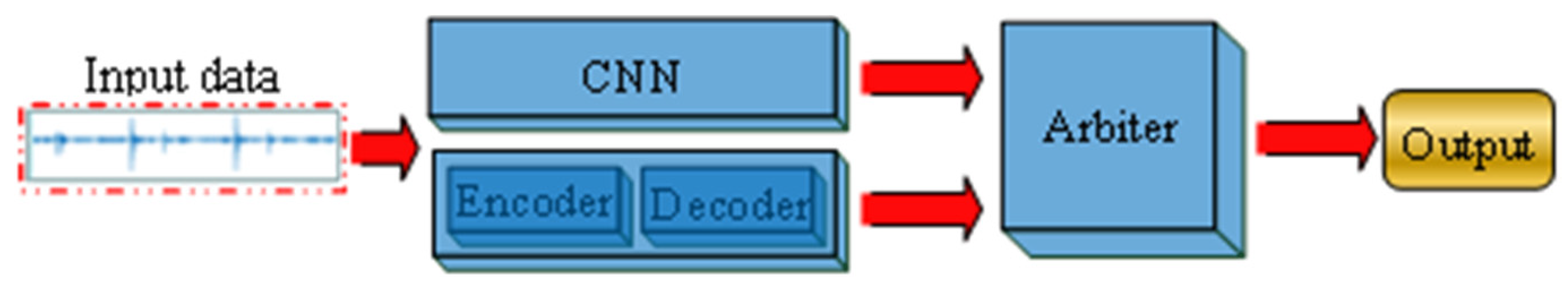
A baseline model for identifying mechanical sub-health states is proposed. Then, the performance of the basic model is improved by adding an auxiliary decision module and using Mahalanobis distance to represent the distances between samples.

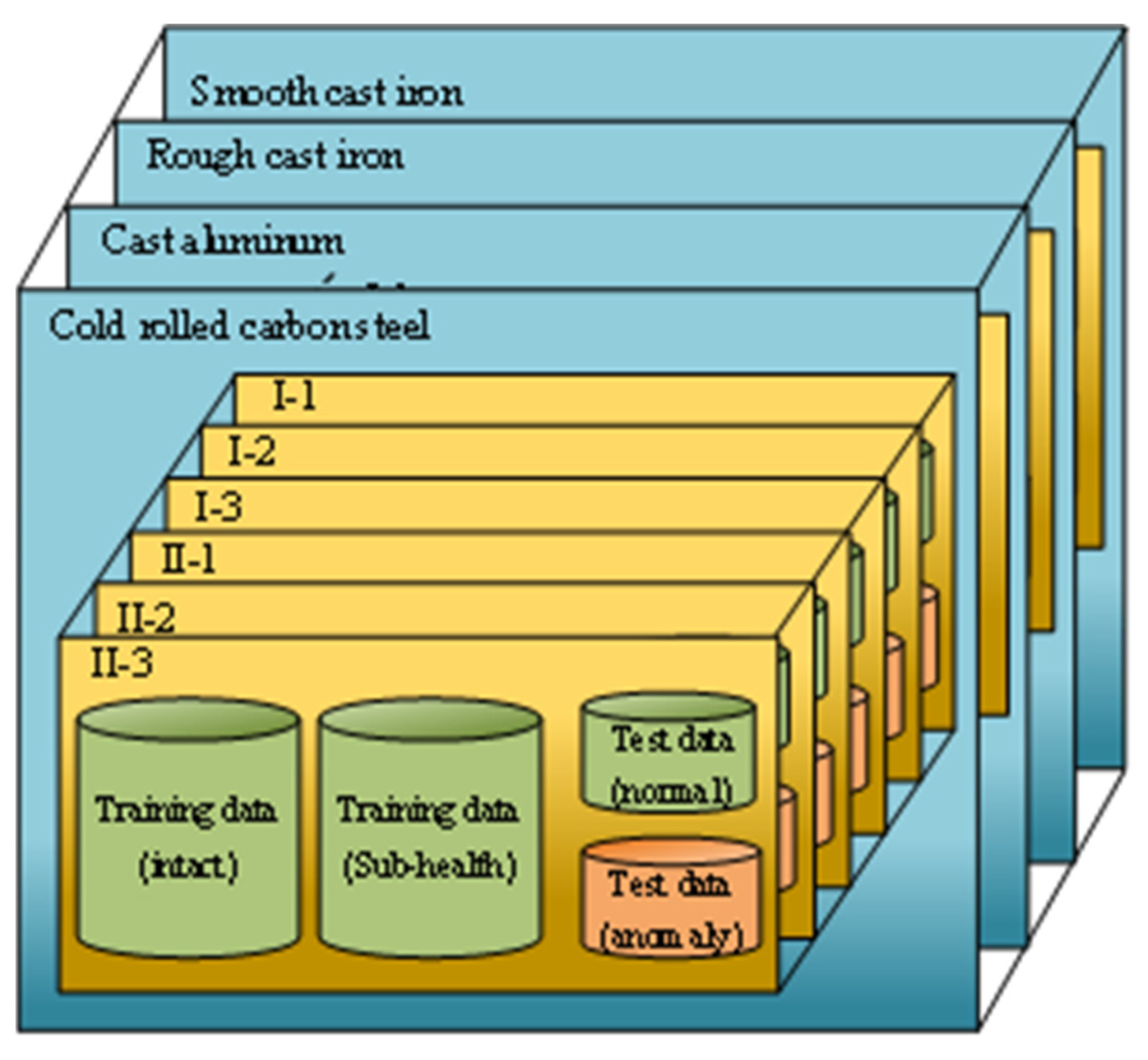
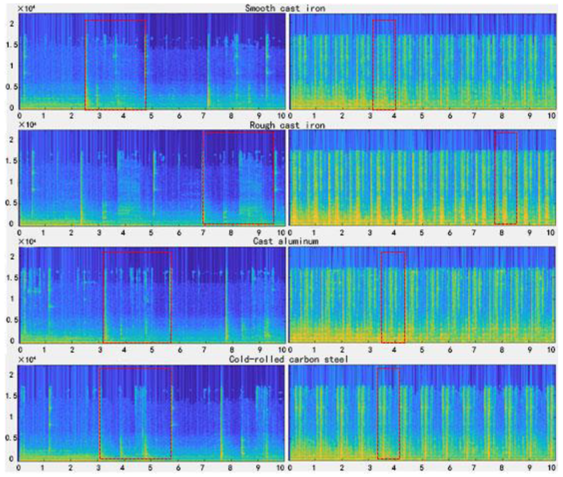
2. Dataset

The dataset we collected is the sound of a traditional mechanical shaping machine when it is working, including the intact sound/sub-healthy sound made by machining four materials in six gears. Each recording is a single channel audio of 10 s, which includes the sounds of the machine, its related equipment, and environmental noise. The four materials are:

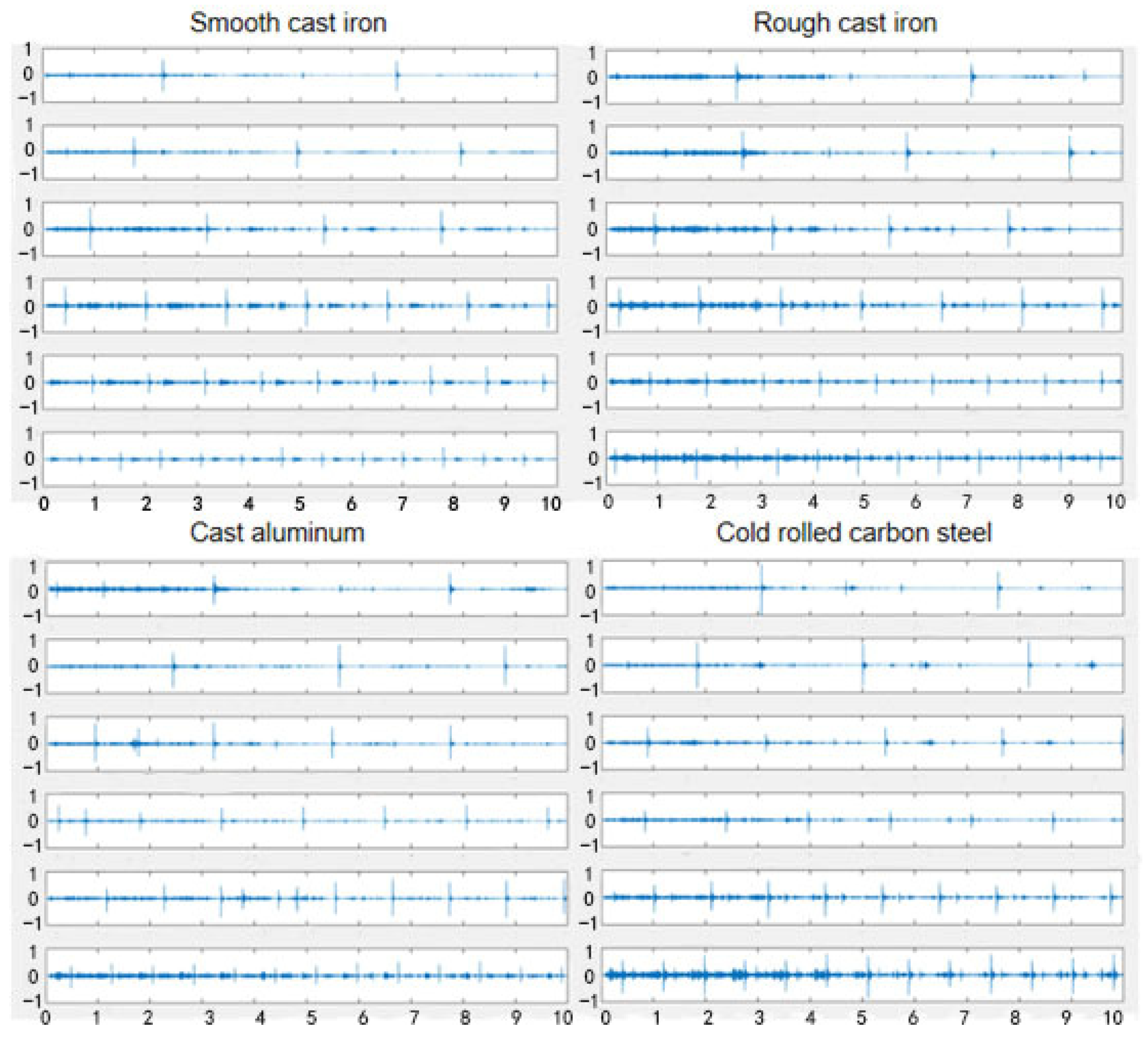
• Smooth cast iron;
• Rough cast iron;
• Cast aluminum;
• Cold-rolled carbon steel.

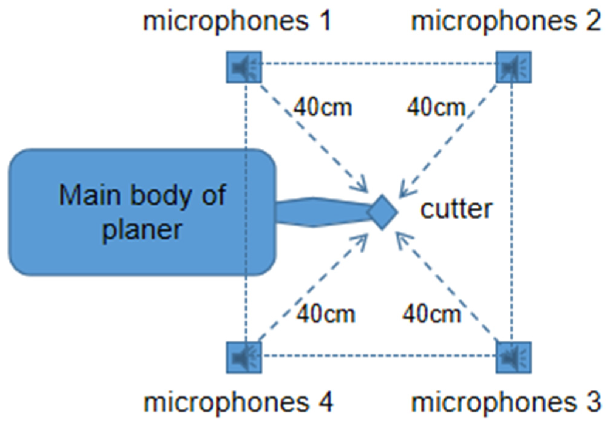
2.1. Recording Process

We use a square microphone array composed of four different microphones to collect sound. The distribution of the microphone array is shown in Figure 1. By using a microphone array, single-channel and multi-channel methods can be evaluated. In order to simplify the task, only the first channel record in the multichannel is used, and multichannel recording will be used in future research. The microphone array was kept at a distance of 40 cm from the machine and recorded a 10 s sound clip. In addition, each machine sound was recorded in a separate session. In the running state, the sound of the machine was recorded as a 16-bit audio signal sampled at 16 kHz in the reverberation environment.

2.2. Introduction to Datasets

As shown in Figure 2, the dataset contains the working sounds of four materials in six gear; each part has a complete training and testing set. Training data include intact data and sub-health data, while test data include normal data and abnormal data. For each part, this dataset provides: (i) intact status data recorded with a new cutter (clips of about 50 normal sounds from the source domain used for training), as shown in Figure 3; (ii) sub-health sample data that were recorded using cutters that were operating continuously for half a year, including 50 sub-health status sounds for training; (iii) abnormal samples data, which were composed of 30 normal sounds with Gaussian distribution and random noise generated by uniform distribution; and (iv) normal sample data, which were about 15 intact and sub-health sample data in the target domain, as shown in Figure 4. In conclusion, each part contained 160 different sound samples, a total of 960 sample data for each material, and 3840 samples were included in the original dataset.

3. Materials and Methods

3.1. Pre-Process and Feature Extration

Pre-processing was divided into four steps. The first step was to pre-emphasize the input digital voice signal in order to emphasize and increase the role of high frequency in the signal and remove the role of influences such as “lip radiation”. The first-order FIR of high-pass digital filter is used to achieve pre-weighting generally, and the transfer function is

$$H\left(Z\right)=1-\alpha z^{-1}$$

(1)

The $\alpha$ is the pre-weighting coefficient with a range of $0.9<\mathsf{\alpha }<1.0$. $x\left(n\right)$ is the value of speech sampling at time $n$, and $y\left(n\right)=x\left(n\right)-\alpha x\left(n-1\right)$ is the result after pre-adding and re-processing, where its value is $\alpha =0.98$.

The second step was sub-frame. In order to make the transition between frames smooth and maintain its continuity, we adopted an overlapping segmentation method. The third step was to add a window and multiply each frame by the Hamming window to increase the continuity between the left and right ends of the frame. Suppose the signal after framing is $S\left(n\right),n=0,1,\cdots ,N-1,N$; then, after obtaining the Hamming window $S^{\prime }\left(n\right)=S\left(n\right)\times W\left(n\right)$, the form $W\left(n\right)$ is as follows:

$$W\left(n,a\right)=\left(1-a\right)-a\times \cos \left[\frac{2\pi n}{N-1}\right],0\le n\le N-1$$

(2)

Different $a$ value will produce different Hamming windows, so we take $a$ value of 0.46.

The fourth step was fast Fourier transform. The time-domain diagram of the data is shown above. It is not easy to ascertain the characteristics of the signal from the diagram. The general method is to perform fast Fourier transform on each frame to attain the energy distribution in the spectrum. Different distributions represent different characteristics.

Finally, the feature collection work was carried out. The feature extraction method we used is currently the most commonly used log-Mel filter in audio processing. The principle of log-Mel is to simulate the structure of the human ear and filter sound. For two sound signals of different loudness, the treble is masked by the bass. Fourier transformation is a step of the entire model, and its purpose is to obtain the energy distribution on the frequency spectrum. Signal energy is used as its basic feature, and signal processing can be used as the output feature. This characteristic is not affected by the nature of the signal, and the corresponding characteristics can be obtained regardless of whether it is treble or bass. This feature has a better recognition effect when the signal-to-noise ratio is low. Figure 5 shows the log-Mel spectrogram of each material we enumerated.

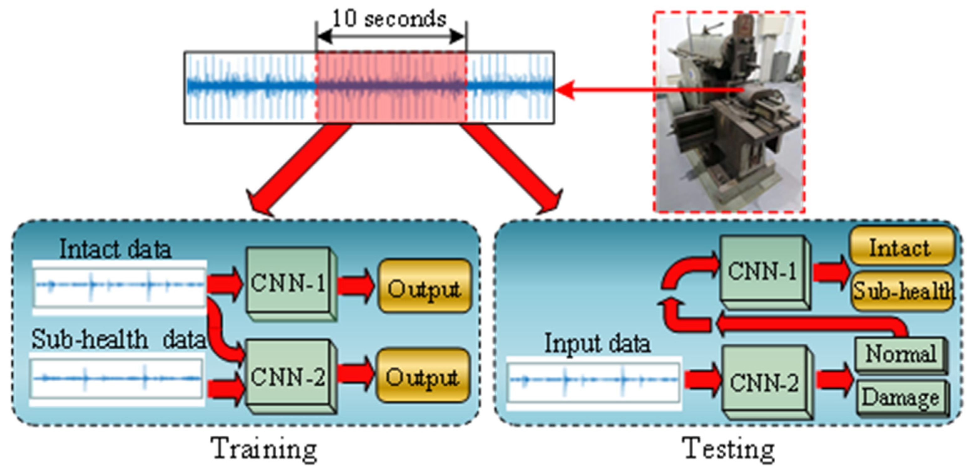
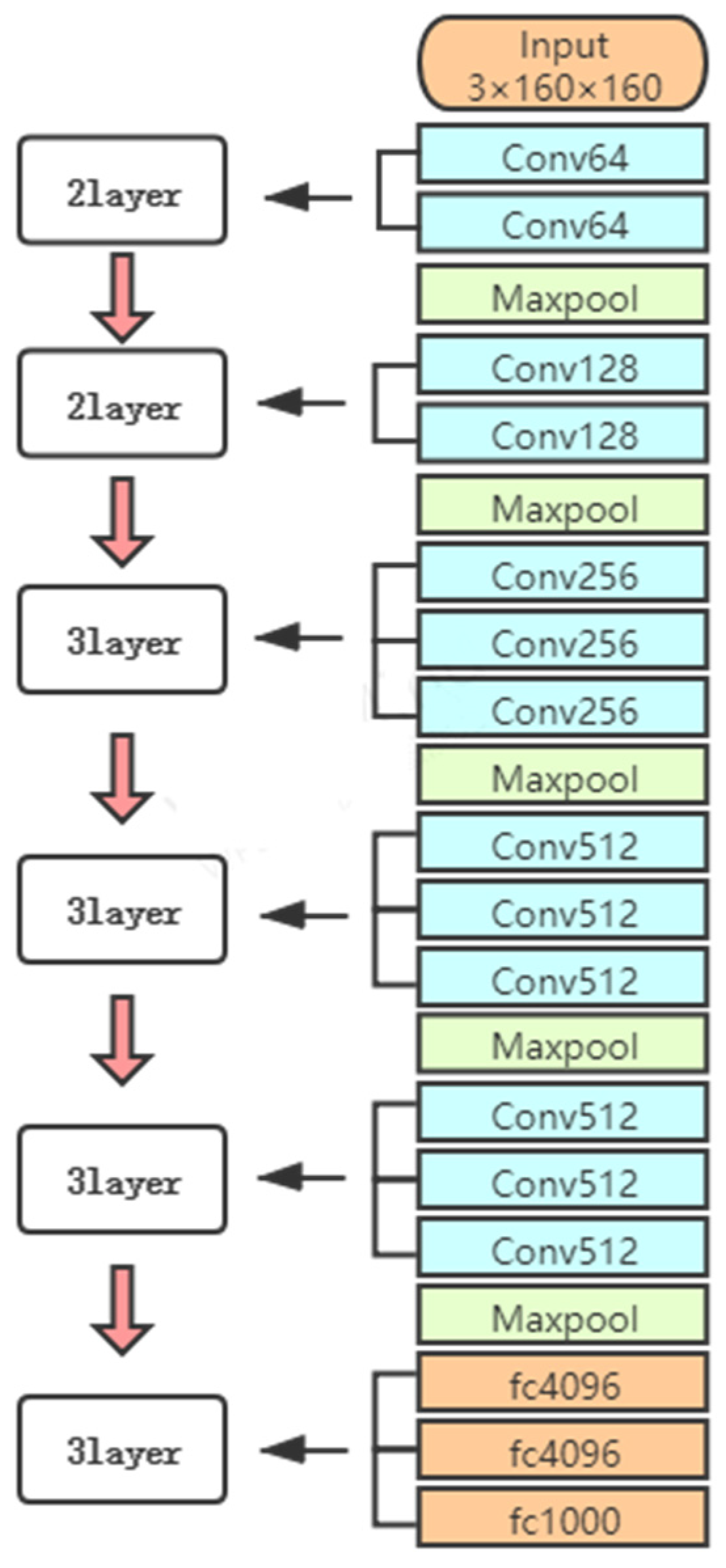
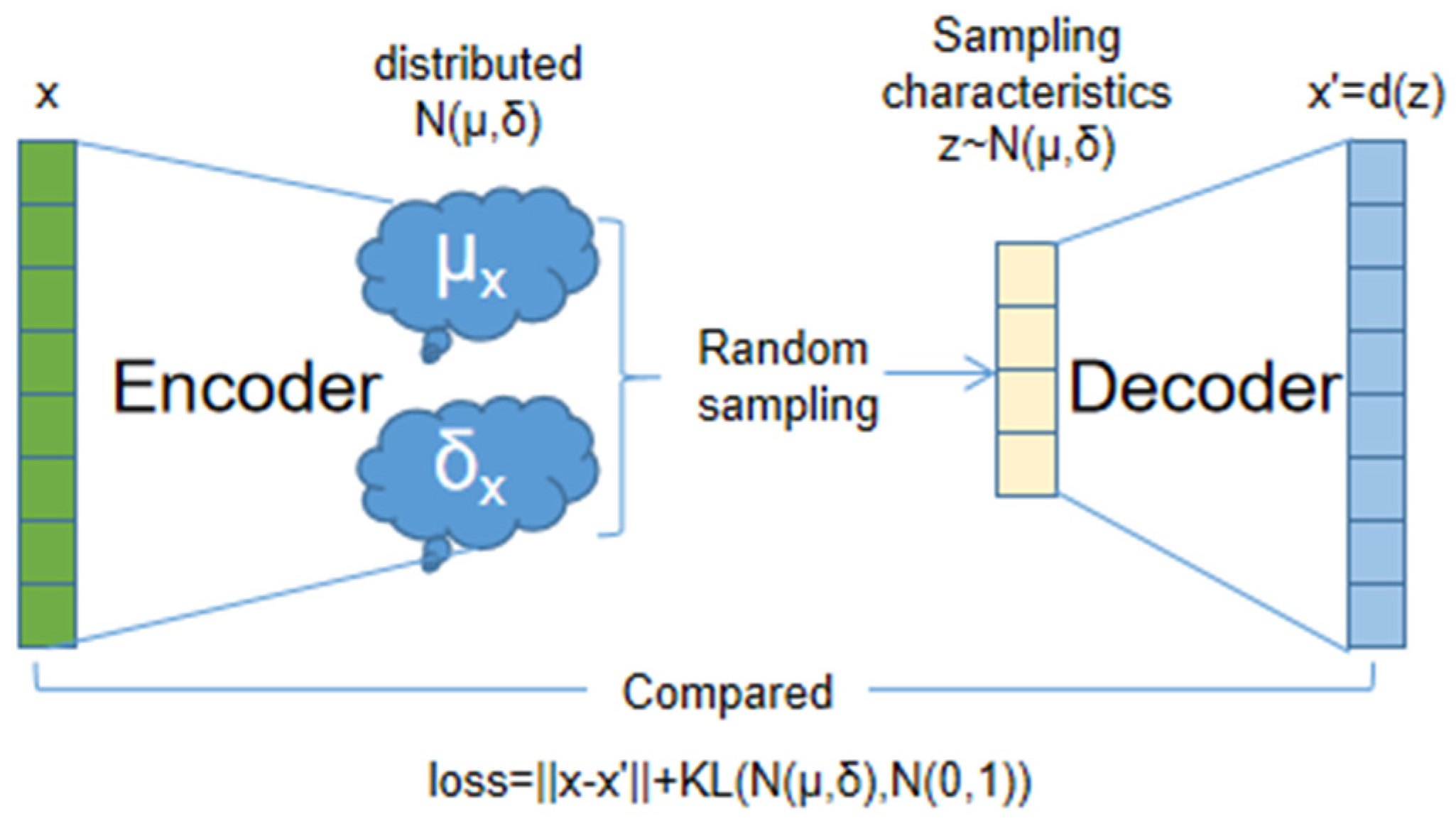
3.2. The Proposed Model

A simple sub-health data recognition model was established by two convolutional neural networks (the flowchart is shown in Figure 6).

In the model, CNN-1 and CNN-2 are exactly the same two VGG16 networks (the network structure is shown in Figure 7). VGG16 [20] contains 13 convolutional layers, 3 fully connected layers, and 5 pool layers. Among them, the convolutional layer and the fully connected layer have weight coefficients, so they are also called weighted layers, and the total number is 16. The convolutional layers all use the same convolution kernel parameters. The size of the convolution kernel used by the convolutional layer (kernel size) is 3; in other words, the width and height are 3, and 3 × 3 is small. The size of the convolution kernel, combined with other parameters (stride = 1, padding = same), enables each convolutional layer (tensor) to maintain the same width and height as the previous layer (tensor).

In training process, intact data are used not only to train the CNN-1 model, but also to train the CNN-2 model, together with sub-health data. The input data in testing would be entered from CNN-2. If they are the normal data that would be entered into the CNN-1 network, it is necessary to determine whether they are sub-health data.

3.3. OOD Detection Principle and Fusion

Hawkins found that, in the actual classification task, many instances of high-confidence prediction resulted in errors. If the classifier cannot advise whenever this error occurs, it can cause serious problems and be limited in practice. Hawkins proved the following experimentally:

(1)

The model can provide a high softmax probability in the OOD samples, and it also has some misclassified samples; in addition, probability cannot directly represent confidence;

(2)

Currently classified samples have a higher softmax probability than misclassified samples and OOD samples.

Therefore, the model shows a difference in softmax prediction probability distribution between the normal classification samples and the OOD samples. By selecting the appropriate threshold, the ID and OOD samples can be distinguished effectively. We incorporate this idea into our model [21,22,23,24,25]. According to the method proposed by OOD detection, we obtained the values of AUPR Succ and AUPR Err (as shown in

Table 1. AUPR is the area under the precision recall curve, reflecting the relationship between precision and recall. Examples of correct classification are treated as positive classes, denoted as Succ; the misclassified example is treated as a positive class, denoted as Err. The “Base” value is obtained using a random detector.

CNN-1		CNN-2
AUPR Succ/base	AUPR Err/base	AUPR Succ/base	AUPR Err/base
91/76	43/24	96/79	62/21

). The large difference between AUPR Succ and AUPR Err in the two networks indicates that the predicted threshold score can be set to detect whether a sample is in the correct range; Wilcoxon rank sum test was used to verify this conclusion.

Finally, we set the output vector of the neural network as $z_1,z_2,\cdots ,z_i$; then, the resulting expression after calculation by the softmax layer was as follows:

$$S_i=\frac{e^{z_i}}{e^{z_1}+e^{z_2}+\cdots +e^{z_i}}{S}_i\in \left[0\%,100\%\right]$$

(3)

If the threshold is set to $Q(1>Q>0.5)$, and the probability of $S_1$ predicted classification obtained through the VGG network is $P$, the final classification result is $\{\begin{array}{c}1\\ 0\end{array}\begin{array}{c}P\ge Q\\ P<Q\end{array}$, where 1 represents in-distribution data and 0 represents OOD data.

3.4. Further Improvements to the Model

In order to achieve better results, we made two more improvements to the base model, which resulted in our final model. The two further improvements are as follows:

Improvement 1: A variational autoencoder auxiliary module added to the network structure (as shown in Figure 8);

Improvement 2: Using Mahalanobis distance to measure the distance between a sample and training data in a manifold space.

An autoencoder is an unsupervised learning algorithm, which is mainly used for data dimension reduction or feature extraction (the structure is shown in Figure 9). The encoder part creates a hidden layer (or multiple hidden layers) containing low dimensional vectors of input data features. The decoder reconstructs the input data through the low dimensional vector of the hidden layer [26]. As we all know, it is easier to distinguish normal samples from abnormal samples in a high-dimensional space, so the output of the decoder greatly improves the decider. The variable autoencoder assumes that the hidden layer after neural network coding is a standard Gaussian distribution; it then samples a feature from the distribution and decodes that feature. The expected result is the same as that of the original input. The loss is almost the same as that of autoencoder, but the regularization term of KL divergence of coding inference distribution and standard Gaussian distribution is increased. The variable autoencoder generates a potential probability distribution $p\left(z|x\right)$ for each input $x$, and then randomly samples from the distribution to obtain a continuous and complete potential space, which solves the problem that the autoencoder cannot be used to generate [27,28,29,30,31,32].

In general, a variable autoencoder is used to add constraints to an encoder, i.e., to force it to produce potential variables that obey the units of Gaussian distribution. One of its advantages is its ability to directly compare differences between reconstructed data and original data, which can play a decisive auxiliary role in our convolutional neural network.

Mahalanobis distance is an effective way to calculate the similarity of two unknown samples as it can measure the distance between points and a distribution [33]. Therefore, we use it to measure the distance between sample $x$ and the ID training data in the manifold space [34,35,36]:

$$D_M\left(x\right)=\sqrt{{(x-\widehat{\mu })}^T{\widehat{{\displaystyle \sum }}}^{-1}\left(x-\widehat{\mu }\right)}$$

(4)

$\widehat{\mu }$ and ${\displaystyle \hat{\sum }}$ are the value of mean and covariance matrices of the multivariate Gaussian distribution. Mahalanobis distance is a constant scale and can also consider the relationship between different dimensions. Finally, using reconstruction error and Mahalanobis distance to detect OOD samples, we find the following:

$$novely\left(x\right)=\alpha \cdot D_M\left(E\left(x\right)\right)+\beta \cdot \lambda \left(x,D_M\left(E\left(x\right)\right)\right)$$

(5)

4. Experiment and Discussion

4.1. Parameter Introduction

There are several fixed detection indicators for OOD detection: true positive rate (TPR), TP, and FN represent true positive and false negative, respectively

$$\mathrm{TPR}=\frac{\mathrm{TP}}{\mathrm{TP}+\mathrm{FN}}$$

(6)

False positive rate (FPR) is calculated in Equation (7), where, FP and TN indicate false positive and true negative, respectively.

$$\mathrm{FPR}=\frac{\mathrm{FP}}{\mathrm{FP}+\mathrm{TN}}$$

(7)

Throughout the experiment, we set two core indicators to measure the performance of our model. These two indicators are AUC value and pAUC value. Area under curve (AUC) represents the ability of the model to distinguish between positive and negative samples, and its value is between 0 and 1. The larger the AUC, the better the performance. pAUC is calculated from a part of the ROC curve within a predetermined range. In our measurements, pAUC was calculated as the AUC with a low false positive rate (FPR) in the range of [0, 0.1]. Thus, pAUC is important for stopping a system from sending out false alarms—it is not trusted, like “The boy who cried wolf”—so we added it into consideration.

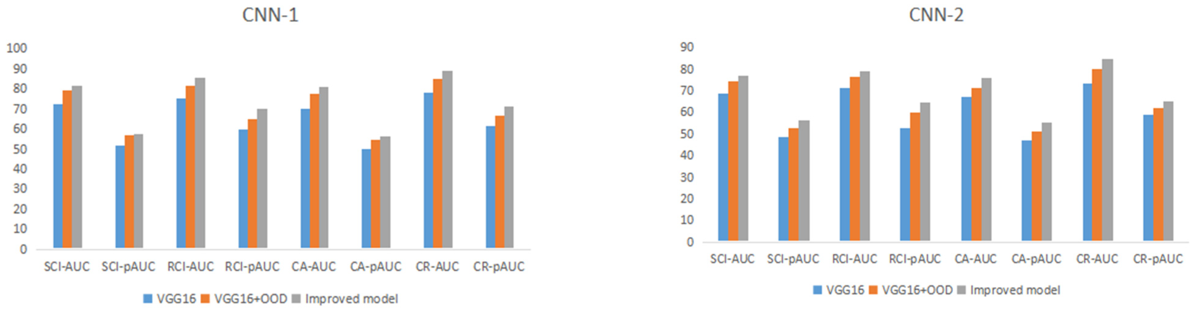
4.2. Results and Discussion

In order to show the effect of OOD detection, we first obtained a group of experimental results that were not integrated into the principle of OOD detection, as shown in

Table 2. Sub-health data recognition results before adding OOD detection.

	Smooth Cast Iron		Rough Cast Iron		Cast Aluminum		Cold-Rolled Carbon Steel
	AUC	pAUC	AUC	pAUC	AUC	pAUC	AUC	pAUC
CNN-1/ Damage	72.31%	51.52%	75.01%	59.77%	69.82%	50.13%	78.29%	61.75%
CNN-2/ Sub-health	68.88%	48.72%	71.49%	53.00%	67.30%	47.08%	73.61%	58.71%

.

The experimental results are shown in Table 2. The average AUCs of the two neural networks in the baseline model were 74.11% and 70.32%, which preliminarily realized the identification of mechanical diagnosis and sub-health state, respectively. Therefore, we prove that it is feasible to judge a mechanical state using sound characteristics when a machine is working.

The experimental results with the addition of the OOD detection method are shown in

Table 3. Sub-health data recognition results after adding OOD detection.

	Smooth Cast Iron		Rough Cast Iron		Cast Aluminum		Cold-Rolled Carbon Steel
	AUC	pAUC	AUC	pAUC	AUC	pAUC	AUC	pAUC
CNN-1/ Damage	79.31%	56.87%	81.70%	64.70%	77.62%	54.89%	85.16%	66.75%
CNN-2/ Sub-health	74.42%	52.53%	76.69%	60.04%	71.12%	51.20%	80.34%	62.29%

. OOD detection only needs to train a network within the distributed data to achieve a suitable classification performance. Moreover, OOD detection is also suitable for detecting mechanical diagnosis with more normal data and fewer abnormal data.

The experimental results show that the improved model is significantly better than the baseline system. Additionally, the average AUCs are 80.95% and 75.64%, respectively, which is 6.84% and 5.32% points higher than the baseline system.

Experimental results of the improved model are shown in

Table 4. Sub-health data recognition results after the addition of auxiliary network.

	Smooth Cast Iron		Rough Cast Iron		Cast Aluminum		Cold-Rolled Carbon Steel
	AUC	pAUC	AUC	pAUC	AUC	pAUC	AUC	pAUC
CNN-1/ Damage	81.74%	57.47%	85.46%	70.10%	80.74%	56.47%	88.92%	71.30%
CNN-2/ Sub-health	76.89%	56.22%	79.32%	64.70%	75.85%	55.54%	84.74%	65.19%

. According to the experimental results, we know that the average AUC of our final model reached 84.22% and 79.20%, which increased by 3.27% and 3.56%, respectively, compared with the previous improvement. The TPR and FPR values of the three experiments are summarized in

Table 5. TPR and FPR results of three experiments. From top to bottom: VGG16 network, VGG16+OOD network, VGG16+OOD+ auxiliary network. All values are in %.

		Smooth Cast Iron		Rough Cast Iron		Cast Aluminum		Cold-Rolled Carbon Steel		Detection Time(s)
		TPR	FPR	TPR	FPR	TPR	FPR	TPR	FPR
1	CNN-1/ Damage	70.4	9.5	71.0	9.6	69.2	8.7	75.5	7.1	323
	CNN-2/ Sub-health	68.9	5.9	69.3	5.5	68.2	6.0	74.7	3.6
2	CNN-1/ Damage	74.5	7.4	74.2	7.4	72.9	8.2	77.3	6.2	384
	CNN-2/ Sub-health	73.7	3.4	72.8	3.9	72.6	4.1	76.7	2.3
3	CNN-1/ Damage	75.8	6.6	76.0	6.5	73.3	8.0	78.1	5.8	571
	CNN-2/ Sub-health	74.4	3.3	73.6	3.4	74.0	3.3	77.6	2.1

. It can be seen from Figure 10 that the model proposed in this paper can effectively identify different states in the dataset by the mechanical sound features, so as to realize the recognition of a mechanical sub-health state; each improvement improves the recognition effect of the model. In addition, it can also be seen that there are obvious differences between the effects of different materials, mainly because of the different hardness and smoothness of the materials, resulting in different degrees of sound characteristics.

4.3. Comparison of Effects under Different Conditions

The dataset based on sound characteristics is only the dataset provided by DCASE 2020 Task 2. This dataset only contains the sound of the machine working normally and the sound after damage. Therefore, it is only possible to compare the effects of mechanical fault diagnosis, as shown in

Table 6. Comparison of mechanical fault identification module and baseline system of DCASE 2020 Task 2. All values are in %.

AUC/pAUC	Fan	Pump	Slider	Valve	ToyCar	ToyConveyor
Baseline	82.80/65.80	82.37/64.11	79.41/58.87	57.37/50.79	80.14/66.17	85.36/66.96
Our model	93.65/82.47	93.68/91.2	97.71/80.55	91.48/89.74	86.06/70.01	88.43/73.44

.

In order to further prove the performance of our proposed method, we added a comparison with two classic neural network models—AlexNet [37] and ResNet [38]. The comparison results are shown in

Table 7. Comparison of the proposed method with other methods. All values are in %.

Sub-Health Identification	Smooth Cast Iron		Rough Cast Iron		Cast Aluminum		Cold-Rolled Carbon Steel
	AUC	pAUC	AUC	pAUC	AUC	pAUC	AUC	pAUC
AlexNet	65.36%	45.71%	67.00%	51.03%	64.52%	44.93%	71.55%	56.87%
ResNet	70.57%	50.76%	71.33%	53.19%	69.21%	50.01%	77.65%	60.14%
Our model	76.89%	56.22%	79.32%	64.70%	75.85%	55.54%	84.74%	65.19%

.

5. Conclusions

In this paper, a method for identifying mechanical sub-health state based on sound characteristics was proposed. By extracting the sound characteristics of the working parts of heavy machinery when working, we solved the problem of poor recognition effects of heavy machinery due to the inconspicuous characteristics of vibration signals. The collected data of the bullhead planer were applied for the recognition experiment of a sub-health state. It was found that a good recognition effect could be achieved by a simple neural network; however, because there were only positive samples, the recognition effect could not be improved further, even if the parameters were continuously modified. Through a fusion experiment with OOD detection, it was found that OOD detection was an effective way to solve a single positive sample; then, the auxiliary decision module and the change in distance representation in its structure could effectively improve the recognition effect. The identification of mechanical sub-health status can ensure the safe operation of equipment, reduce maintenance costs, and prevent the occurrence of major accidents. Therefore, sub-health detection is more practical than fault detection. In future work, we will use a more efficient and precise neural network model and a more reasonable framework to improve accuracy and efficiency, and we will draw on more ideas to continuously improve the efficacy of our model’s recognition.

References

- Zhang, A.; Li, S.; Cui, Y.; Yang, W. Limited Data Rolling Bearing Fault Diagnosis with Few-Shot Learning. IEEE Access 2019, 7, 110895–110904. [Google Scholar] [CrossRef]
- Zhang, W.; Peng, G.; Li, C.; Chen, Y.; Zhang, Z. A new deep learning model for fault diagnosis with good anti-noise and domain adaptation ability on raw vibration signals. Sensors 2017, 17, 425. [Google Scholar] [CrossRef]
- Hang, Q.; Yang, J.; Xing, L. Diagnosis of rolling bearing based on classification for high dimensional unbalanced data. IEEE Access 2019, 7, 79159–79172. [Google Scholar] [CrossRef]
- Sun, W.; Shao, S.; Zhao, R.; Yan, R.; Zhang, X.; Chen, X. A sparse auto-encoder-based deep neural network approach for induction motor faults classification. Measurement 2016, 89, 171–178. [Google Scholar] [CrossRef]
- Yiallourides, C.; Naylor, P.A. Time-Frequency Analysis and Parameterisation of Knee Sounds for Non-invasive Detection of Osteoarthritis. IEEE. Trans. Biomed. Eng. 2021, 68, 1250–1261. [Google Scholar] [CrossRef]
- Das, S.; Pal, S.; Mitra, M. Acoustic feature based unsupervised approach of heart sound event detection. Comput. Biol. Med. 2020, 126, 103990–104000. [Google Scholar] [CrossRef] [PubMed]
- Bayram, B.; Duman, T.B.; Ince, G. Real time detection of acoustic anomalies in industrial processes using sequential autoencoders. Expert Syst. J. Knowl. Eng. 2020, 38, e12564. [Google Scholar] [CrossRef]
- Liu, L.; Li, B.; Zhao, R.; Yao, W.; Shen, M.; Yang, J. A Novel Method for Broiler Abnormal Sound Detection Using WMFCC and HMM. J. Sens. 2020, 2020, 2985478. [Google Scholar] [CrossRef] [Green Version]
- Tran, T.; Lundgren, J. Drill Fault Diagnosis Based on the Scalogram and Mel Spectrogram of Sound Signals Using Artificial Intelligence. IEEE Access 2020, 8, 203655–203666. [Google Scholar] [CrossRef]
- Wang, F.; Lin, W.; Liu, Z.; Qiu, X. Pipeline Leak Detection and Location Based on Model-Free Isolation of Abnormal Acoustic Signals. Energies 2019, 12, 3172. [Google Scholar] [CrossRef] [Green Version]
- Volkmann, N.; Kulig, B.; Kemper, N. Using the Footfall Sound of Dairy Cows for Detecting Claw Lesions. Animals 2019, 9, 78. [Google Scholar] [CrossRef] [Green Version]
- Hou, C.; Qiao, T.; Qiao, M.; Xiong, X.; Yang, Y. Research on Audio-Visual Detection Method for Conveyor Belt Longitudinal Tear. IEEE Access 2019, 7, 120202–120213. [Google Scholar] [CrossRef]
- Ramteke, S.M.; Chelladurai, H.; Amarnath, M. Diagnosis of Liner Scuffing Fault of a Diesel Engine via Vibration and Acoustic Emission Analysis. J. Vib. Eng. Technol. 2019, 8, 815–833. [Google Scholar] [CrossRef]
- Hendrycks, D.; Gimple, K. A Baseline for Detecting Misclassified and Out-of-Distribution Examples in Neural Networks. arXiv 2017, arXiv:1610.02136. [Google Scholar]
- Liang, S.; Li, Y.; Srikant, R. Principled Detection of Out-of-Distribution Examples in Neural Networks. arXiv 2017, arXiv:1706.02690. [Google Scholar]
- Devries, T.; Taylor, G.W. Learning Confidence for Out-of-Distribution Detection in Neural Networks. arXiv 2018, arXiv:1802.04865. [Google Scholar]
- Shalev, G.; Adi, Y.; Keshet, J. Out-of-Distribution Detection using Multiple Semantic Label Representations. In Proceedings of the 32nd Conference on Neural Information Processing Systems (NIPS), Montreal, QC, Canada, 2–8 December 2018; Volume 31, pp. 1–11. [Google Scholar]
- Denouden, T.; Salay, R.; Czarnecki, K.; Abdelzad, V. Improving Reconstruction Autoencoder Out-of-distribution Detection with Mahalanobis Distance. arXiv 2018, arXiv:1812.02765. [Google Scholar]
- Abdelzad, V.; Czarnecki, K.; Salay, R. Detecting Out-of-Distribution Inputs in Deep Neural Networks Using an Early-Layer Output. arXiv 2019, arXiv:1910.10307. [Google Scholar]
- Simonyan, K.; Zisserman, A. Very Deep Convolutional Networks for Large-Scale Image Recognition. arXiv 2015, arXiv:1409.1556. [Google Scholar]
- Asami, T.; Masumura, R.; Aono, Y.; Shinoda, K. Recurrent out-of-vocabulary word detection based on distribution of features. Comput. Speech Lang. 2019, 58, 247–259. [Google Scholar] [CrossRef]
- Berend, D.; Xie, X.; Ma, L.; Zhou, L.; Liu, Y.; Xu, C.; Zhao, J. Cats Are Not Fish: Deep Learning Testing Calls for Out-Of-Distribution Awareness. In Proceedings of the 2020 35th IEEE/ACM International Conference on Automated Software Engineering (ASE), Melbourne, VIC, Australia, 21–25 September 2020; pp. 1041–1052. [Google Scholar]
- Gal, Y.; Ghahramani, Z. Dropout as a bayesian approximation: Representing model uncertainty in deep learning. In Proceedings of the 33rd International Conference on Machine Learning, ICML, New York, NY, USA, 19–24 June 2016; Volume 6, pp. 1651–1660. [Google Scholar]
- Henriksson, P.; Berger, C.; Borg, M.; Tornberg, L.; Raman, S. Performance Analysis of Out-of-Distribution Detection on Various Trained Neural Networks. In Proceedings of the 2019 45th Euromicro Conference on Software Engineering and Advanced Applications (SEAA), Kallithes, Greece, 28–30 August 2019; pp. 113–120. [Google Scholar]
- Kim, Y.; Cho, D.; Lee, J. Wafer Map Classifier using Deep Learning for Detecting Out-of-Distribution Failure Patterns. In Proceedings of the 2020 IEEE International Symposium on the Physical and Failure Analysis of Integrated Circuits (IPFA), Singapore, 20–23 July 2020; pp. 1–5. [Google Scholar]
- Jia, G.; Liu, G.; Yuan, Z.; Wu, J. An Anomaly Detection Framework Based on Autoencoder and Nearest Neighbor. In Proceedings of the 2018 15th International Conference on Service Systems and Service Management (ICSSSM), Hangzhou, China, 21–22 July 2018; pp. 1–6. [Google Scholar]
- McInnes, L.; Healy, J.; Saul, N.; Grossberger, L. Umap: Uniform manifold approximation and projection. J. Open Source Softw. 2018, 3, 861–923. [Google Scholar] [CrossRef]
- Chen, X.; Kingma, D.P.; Salimans, T.; Duan, Y.; Dhariwal, P.; Schulman, J.; Sutskever, I.; Abbeel, P. Variational Lossy Autoencoder. arXiv 2017, arXiv:1611.02731. [Google Scholar]
- Deng, J.; Zhang, Z.; Eyben, F.; Schuller, B. Autoencoder-based Unsupervised Domain Adaptation for Speech Emotion Recognition. IEEE Signal Process. Lett. 2014, 21, 1068–1072. [Google Scholar] [CrossRef]
- Hou, X.; Shen, L.; Ke, S.; Qiu, G.D. Deep Feature Consistent Variational Autoencoder. In Proceedings of the 2017 IEEE Winter Conference on Applications of Computer Vision (WACV), Santa Rosa, CA, USA, 24–31 March 2017; pp. 1133–1141. [Google Scholar]
- Bando, Y.; Mimura, M.; Itoyama, K.; Yoshii, K.; Kawahara, T. Statistical Speech Enhancement Based on Probabilistic Integration of Variational Autoencoder and Non-Negative Matrix Factorization. In Proceedings of the 2018 IEEE Onternational Conference on Acoustice, Speech and Signal Processing (ICASSP), Calgary, AB, Canada, 15–20 April 2018; pp. 716–720. [Google Scholar]
- Suh, S.; Chae, D.H.; Kang, H.-G.; Choi, S. Echo-state conditional variational autoencoder for anomaly detection. In Proceedings of the 2016 International Joint Conference on Neural Networks (IJCNN), Vancouver, BC, Canada, 24–29 July 2016; pp. 1015–1022. [Google Scholar]
- Maesschalck, R.D.; Jouan-Rimbaud, D.; Massart, D.L. The Mahalanobis distance. Chemom. Intell. Lab. Syst. 2000, 50, 1–18. [Google Scholar] [CrossRef]
- Vareldzhan, G.; Yurkov, K.; Ushenin, K. Anomaly Detection in Image Datasets Using Convolutional Neural Networks, Center Loss, and Mahalanobis Distance. arXiv 2021, arXiv:2104.06193. [Google Scholar]
- Sarmadi, H.; Karamodin, A. A novel anomaly detection method based on adaptive Mahalanobis-squared distance and one-class kNN rule for structural health monitoring under environmental effects. Mech. Syst. Signal Process. 2020, 140, 106495. [Google Scholar] [CrossRef]
- Kamoi, R.; Kobayashi, K. Why is the Mahalanobis Distance Effective for Anomaly Detection. arXiv 2020, arXiv:2003.00402. [Google Scholar]
- Krizhevsky, A.; Sutskever, I.; Hinton, G.E. ImageNet classification with deep convolutional neural networks. Commun. ACM 2017, 60, 84–90. [Google Scholar] [CrossRef]
- He, K.; Zhang, X.; Ren, S.; Sun, J. Deep residual learning for image recognition. In Proceedings of the IEEE Conference on Computer Vision and Pattern Recognition (CVPR), Las Vegas, NV, USA, 27–30 June 2016; pp. 770–778. [Google Scholar] [CrossRef] [Green Version]