1. Introduction
The Cartesian structure is widely used in robotics and automatic machines. The Cartesian structure offers some advantages, since it is stiffer than a jointed arm structure and kinematically simpler. In many applications, the Cartesian structure can be very large with strokes of many meters and may experience very large accelerations. In other applications, the tool mounted on the Cartesian structure may generate large forces or high frequency vibrations that increase noise emission. In these conditions, the analysis and control of vibrations becomes an important issue for a Cartesian structure, as well.
The first research studies on this topic were carried out in the last few years of the past century by some authors that highlighted the configuration-dependent vibration characteristics of these machines [
1,
2] and the effect of the modes of vibration of the structural elements on the robot’s performance [
1]. A detailed review on dynamic analysis of robots with flexible links can be found in Reference [
3]. In Reference [
4], modal analysis techniques were adopted to study the dynamic response of a high speed Cartesian robot excited by severe inertia forces. In Reference [
5], the problem of analyzing the configuration-dependent natural frequencies of a Cartesian Robot was tackled using a FE model to perform simulations in a discrete number of points of the workspace and a regression algorithm to estimate the continuous distribution of natural frequencies.
Today, there are various methods for the dynamic analysis of flexible Cartesian robot, which can be grouped into three families: the FE based methods, the Jacobian methods and the matrix structural analysis (MSA) methods [
6,
7].
The FE methods, such as in Reference [
5], are based on FE analysis of the components of the robot, they may lead to cumbersome numerical models. The Jacobian methods are based on the Jacobian matrix and on compliant virtual joints that mimic the actual compliance of the machine [
8,
9]. MSA methods are similar to the FE methods, but make use of larger elements obtained by means of static condensation [
7,
10]; this approach reduces the computational burden of FE methods, but may require complex mathematical manipulations.
In recent years, many studies focused also on the development of control strategies able to achieve in Cartesian robots position control and vibration damping at the same time [
11,
12]. In particular, in Reference [
13], a specific non-linear control was developed to dampen the vibrations of the end-effector caused by the flexibility of the last link and by fast motion in a perpendicular direction. A similar problem was tackled in Reference [
12], since each subsystem of a Tripteron robot was modeled as a flexible link driven by a prismatic actuator. In the same way, Reference [
14] focused on a control strategy that allows vibration avoidance, but this approach is suitable only for machines that operate with point-to-point movements; in Reference [
15], a control strategy was applied to cornering applications (i.e., the movement of a Cartesian machine where speed direction changes are required). Finally, in Reference [
16], a Cartesian-guided tripod dynamic model was studied, and the vibrations were damped by means of a control strategy.
This paper addresses a different problem: the reduction of high frequency vibrations generated by a pneumatic tool mounted on the last link of a Cartesian cutting machine. In this case, the motion caused by the prismatic actuators of the machine does not generate vibrations of the last link but can lead to variations in the response of the structure to high frequency vibrations, since the workspace is rather large, and beam flexibility is not negligible.
The complexity of the Cartesian machine is reduced by means of a mathematical model adopting a subsystem approach, which aims to model each component of the machine with the simplest model that retains the main characteristics of the component. This model can be used to simulate different machines and for specific actions, such as structural modifications. The cutting head is modeled as an equivalent robotic system with lumped compliances that mimic the actual compliance properties that were experimentally identified. This approach is similar to the aforementioned Jacobian methods [
9]. The moving rail, which has a limited cross section in order to reduce the inertial effects on the actuators, is modeled as a flexible continuous system with the mode superposition approach. Finally, a global analytical model is obtained coupling the aforementioned models and is solved in MATLAB.
The paper is organized as follows.
In the next section, the Cartesian cutting machine is described, and the vibration control problem is stated.
The mathematical model of the machine is developed and discussed in
Section 3.
In
Section 4, experimental tests are presented; they are aimed at identifying the properties of the subsystems of the machine and are carried out with a specific modal analysis approach (selective modal analysis [
17]) that allows separation of the contributions of the various machine subsystems.
In
Section 5, a best fitting method is used to identify model parameters from experimental tests; then, the model is validated.
In
Section 6, the model is used for analyzing the influence of the modes of vibration of the Cartesian structure on the dynamic response of the cutting head.
In
Section 7, the mathematical model is used for assessing the effectiveness of a tuned vibration absorber (TVA), designed to cancel the main resonance of the cutting head.
2. The Cartesian Cutting Machine
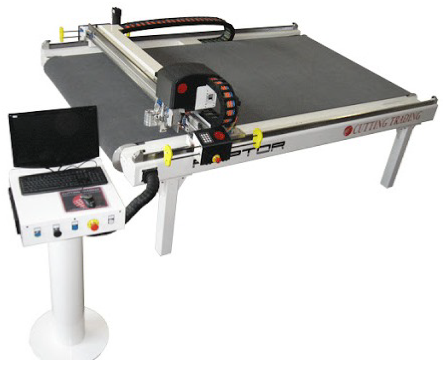
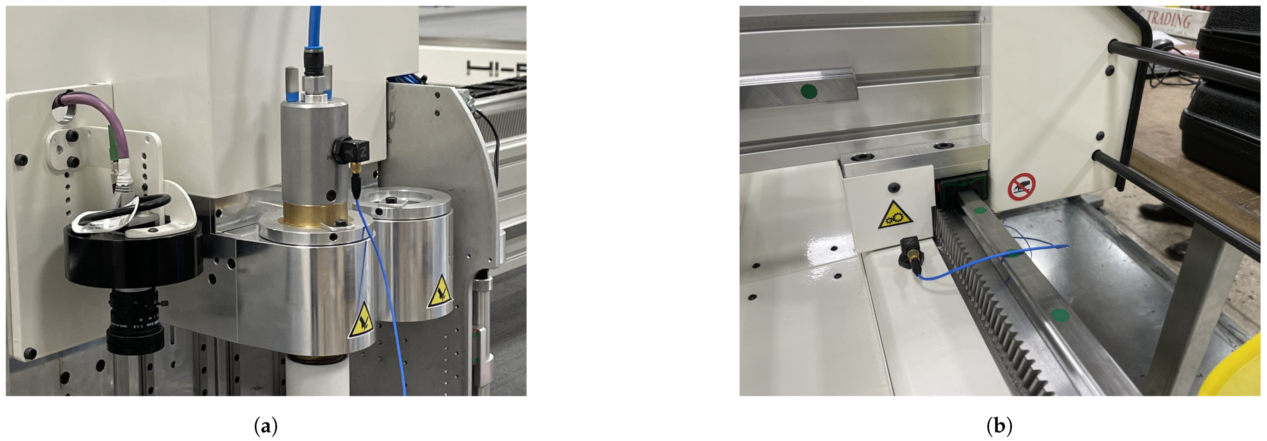
The machine considered in this work is built to cut sheets of different materials, particularly cloth ones. The machine can be seen in
Figure 1.
It is constituted of a Cartesian machine that operates over a conveyor belt, supported by four (4) pillars. The sheets are unrolled over the belt and are cut by a cutting head mounted on the moving rail. This rail is supported at both sides by linear guides. Electric motors coupled to elliptical racks drive the moving rail and the cutting head, which are supported by ball bearing guides. The presence of cables and their support should be taken into account, since they can involve different responses to vibrations on each side of the sliding rail.
The cutting tool moves in the vertical direction and is controlled by means of a pneumatic system that, by means of a valve at the input of the tool, inflates and deflates at high frequency air inside a cylinder. This mechanism can guarantee high cutting speed but, at the same time, generates vibrations that may cause annoying noise, especially at high frequencies.
The machine is modular, so it can be sized to overcome different customer needs.
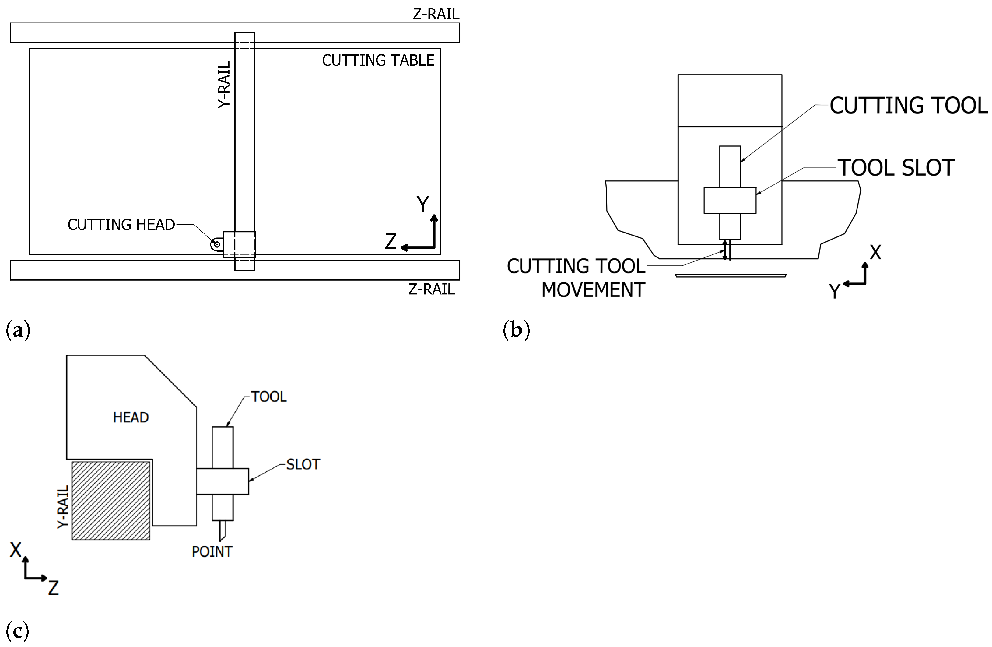
Figure 2 shows a simplified scheme of the cutting machine. The cutting head is rather bulky and is supported by ball bearings. The cutting tool is connected to the head by means of a cantilevered slot. This design allows a quick replacement of the cutting tool, which is very useful, but slot deformability makes possible a rotation of the tool with respect to the head in the presence of an eccentric cutting force.
The moving Y-rail has to operate at high speed in order to improve productivity; for this reason, it is made of an aluminum profile having a limited cross section. Therefore, the influence of the deformability of the moving rail has to be taken into account in the model of the machine.
Conversely, the Z-rails, which are fixed, are made of steel and are very bulky and stiff. There are no practical and theoretical reasons that limit the stiffness of the fixed rails, their cross section can be further increased, if needed, and the number of supports can be increased, if a larger machine has to be developed.
It is worth noticing that most of the aforementioned characteristics (e.g., the large stiffness of the fixed rails) can be generalized to other Cartesian cutting machines extending the validity of the developed model.
Some preliminary experimental tests showed the main features of the vibrations of this machine [
18]:
the presence of an important periodic force in the vertical direction with fundamental frequency of 217 Hz, caused by the operation of the cutting tool;
the presence of two resonances of the tool at 215 and 248 Hz, respectively, and vibrations at these frequencies showed the largest amplitudes in the vertical direction, relevant amplitudes in the Z direction, negligible amplitudes in the Y direction, and a coupling between the X and Z directions; and
the variation of measured vibrations in the workspace of the machine.
3. Mathematical Model
The mathematical model aims at predicting the response of the cutting machine in the frequency band that includes the maximum excitation for every configuration of the Cartesian robot. The whole cutting machine is divided into two subsystems: the cutting head and the moving rail.
3.1. Cutting Head Model
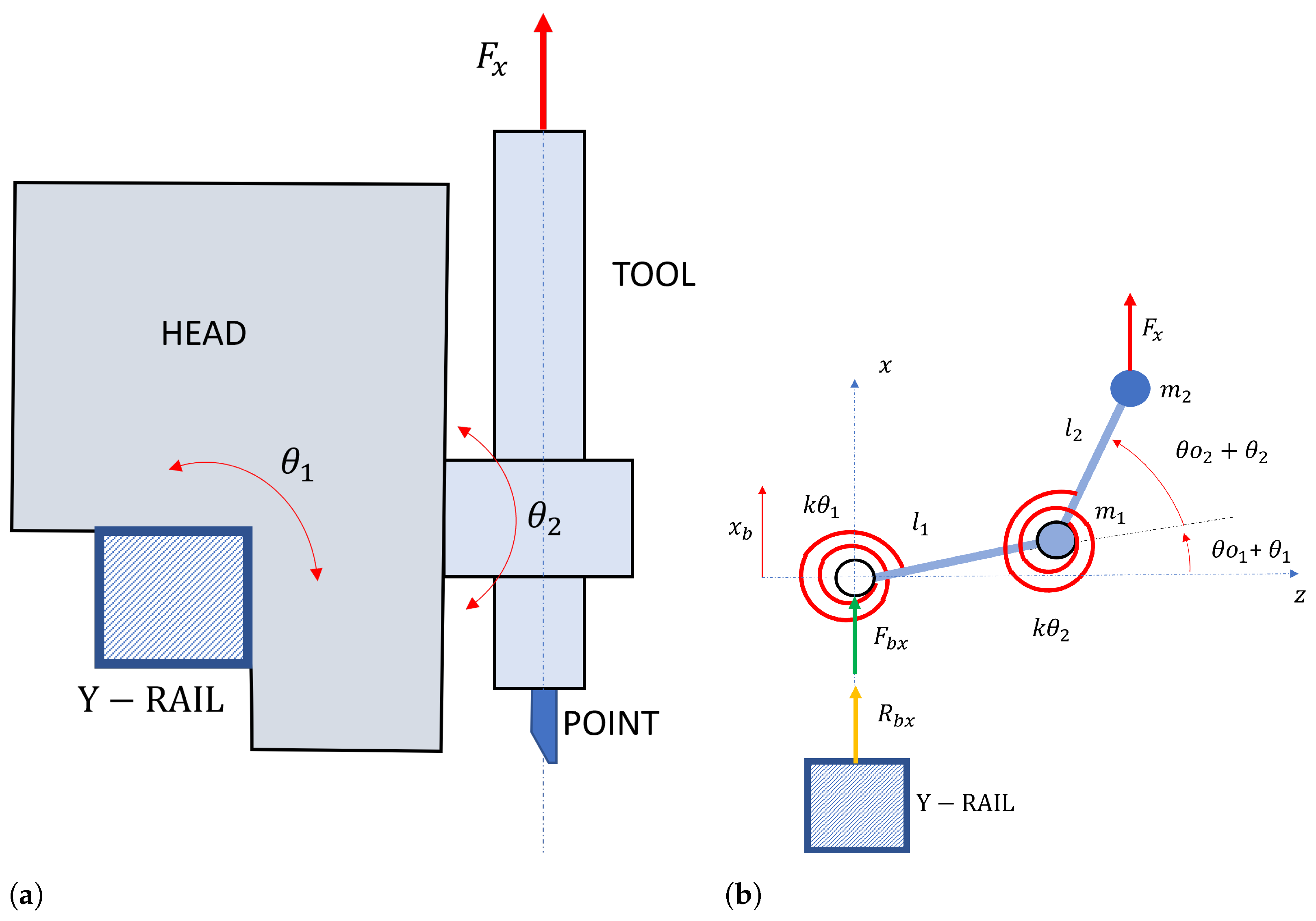
The preliminary tests reported in Reference [
18] showed vibrations in the X and Z directions. They can be related to bending of the moving rail, to slot deformation that leads to a rotation of the tool (rotation
in
Figure 3a), and to bearings compliance that leads to a rotation of the cutting head (rotation
in
Figure 3a) The definition of the centers of rotation is very difficult, since they are related to the specific deformation pattern. Therefore, adopting a grey box approach, the cutting head is modeled as an equivalent jointed-arm robot having 3 Degrees of Freedom; see
Figure 3.
Two DOFs are associated to rotations
and
of the joints with respect to the reference configuration, and the third DOF is associated to vertical translation of the robot base
, which is due to the compliance of the rail. The two links having lengths
and
are mass-less and have two tip masses (
and
, respectively). Two torsional springs (
and
) represent joint compliance. In parallel with the springs, there are two rotational dampers (with damping coefficients
and
), which represent joint damping and are not shown in
Figure 3. Stiffness
is related to the stiffness of the cutting head and to the stiffness of the bearing of the prismatic joint between the Y-rail and the cutting head. Mass
is related to the mass of the cutting head. Stiffness
is chiefly related to the connection between the cutting head and the tool, and mass
is related to the mass of the tool. The joint variables that define the reference configuration of the vibrating robot are important. In particular, joint variable
chiefly defines the ratio between vertical (X) and longitudinal (Z) accelerations, whereas joint variable
, which is the relative angle between link 2 and link 1 in the reference condition, defines the importance of the inertial cross coupling between the joints [
19].
The adopted robotic model is more suitable than a linear model consisting of two lumped masses moving along the X and Z directions, since, in this model, vibrations in the X and Z directions would be completely un-coupled. This behavior is not realistic in the present case, since the compliances of the cutting head generate two rotations in the vertical plane causing coupled displacements in the X and Z directions.
Two external forces act on the equivalent robot. Force is the force in the vertical direction caused by the cutting process, whereas force is the force exerted by the Y-rail on the cutting head.
The equations of motion are derived with the Lagrange method and are expressed in matrix form, and gravity forces are neglected:
Mass matrix is symmetric and includes the inertial cross-coupling terms (the terms outside diagonal):
The damping and stiffness matrices are simple diagonal matrices. The vector at the right-hand side includes the effect of the cutting force and of the reaction force that the Y-rail exerts on the cutting head.
There are four unknowns: , , , and .
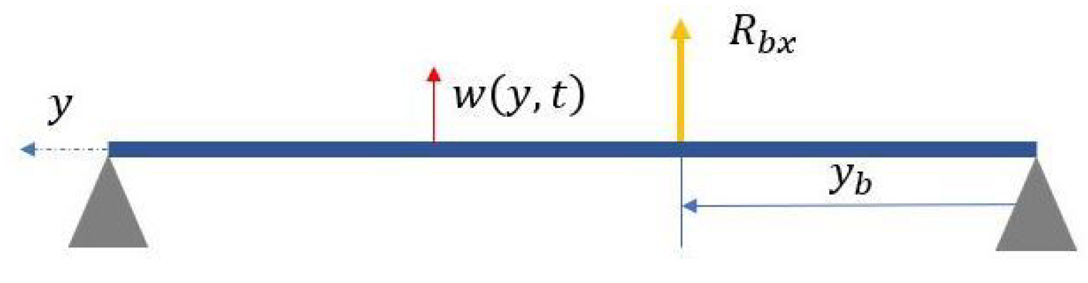
3.2. Y-Rail Model
Figure 4 represents the model of the moving Y-rail in the vertical plane X-Z that contains the excitation force due to the cutting process (in X direction).
The Y-rail, which dominates the vibrational behavior of the Cartesian robot, is modeled as a distributed parameter system by this equation:
where
is the vertical displacement of any point along the Y-rail,
is the bending stiffness of the cross-section of the rail,
is the mass per unit length, and
is the strain-rate damping coefficient. At the right-hand side, there is the forcing term due to the interaction with the cutting head, which is located in position
:
and
is the Dirac delta function.
It is worth noticing that the displacement of the robot base is:
Displacement
can be expressed according to the mode superposition approach as:
where
is the r-th modal coordinate, and
is the r-th mass-normalized mode of vibration. The modes of vibration can be obtained solving the free vibration problem with proper boundary conditions, which are pinned ends in the present case, since the Z-rails can be considered rigid bodies. These modes of vibration hold true even if the beam is proportionally damped. The modes of vibration are associated with the natural frequencies:
where
L is rail length.
If (
7) is inserted into (
4), the equation of forced vibrations is transformed into a set of second order ordinary differential equations:
in which
is modal damping ratio. Actually, if only
m modes of vibration of the Y-rail belong to the frequency band of interest, the vibration of the Y-rail can be represented by
m equation, such as (
9).
3.3. Coupled Model
The model of the equivalent robot is coupled with the model of the beam, considering that:
A system of linear differential equations in unknowns is obtained, the unknowns being , , , , …, .
Since the third equation of the equivalent robot makes it possible to express
as a function of the other variables, a final system of
linear differential equations in
unknowns is obtained. The system is recast in matrix form and implemented in MATLAB. Then, a harmonic forcing function in x direction is used to calculate the forced response:
where
and
are the amplitude and frequency of the cutting force.
The frequency response functions between the coordinates (physical and modal) and the cutting force are calculated solving the linear system with
in the range
. The FRFs between X and Z displacements of the tool are calculated according to the following equations:
where
and
are the FRFs between the rotations
,
, and the cutting force in the X-direction, whereas
is the FRF between the displacement
and the cutting force.
The cutting force in x direction shows a small eccentricity with respect to the center of the Y-beam; therefore, further studies will include the effect of torsion deformability, as well.
4. Experimental Tests
The dynamic properties of the cutting machine have been identified with the selective modal analysis approach [
17,
20,
21]. This method aims at finding particular configurations of the machine in which only the stiffness properties of a specific subsystem (a joint or a flexible link) are important. In the present case, the Frequency Response Fuctions of the cutting head are measured when the cutting head is located at the border of the workspace and nearly above one of the steel pillars that support the rails. This configuration minimizes the influence of bending deformability of rails.
The tests were carried out using an instrumented hammer for modal testing (PCB 086C03) and a triaxial accelerometer (PCB 356A17) with sensitivities of and , respectively. The signals from the hammer and the accelerometer were acquired by means of the DAQ module NI 9234, using the software Signal Express. The sampling rate in the time domain was set to 4000 Hz, whereas the frequency resolution was 0.5 Hz. The PSD of the hammer force showed relevant amplitudes in the range of frequency of interest and the first minimum above 400 Hz.
The measurement points were defined both on the tool and on the rails of the Cartesian machine (
Figure 5). This is due to the necessity of assessing the influence of the machine components on the vibrations of the tool.
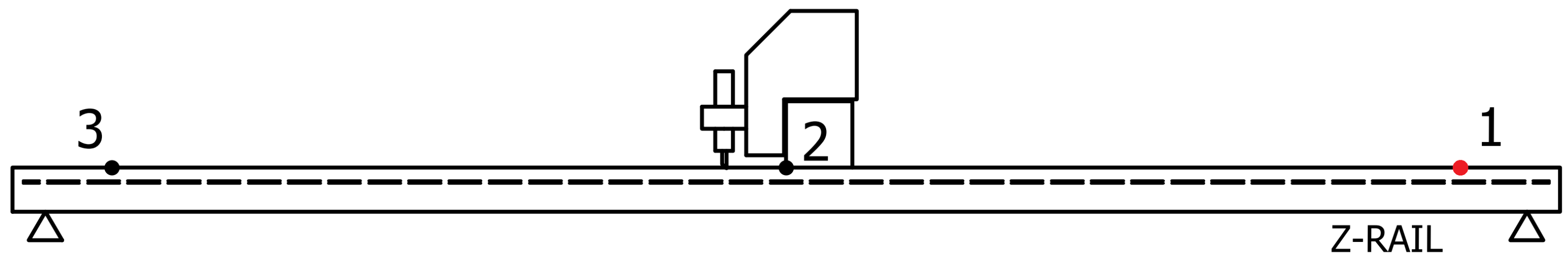
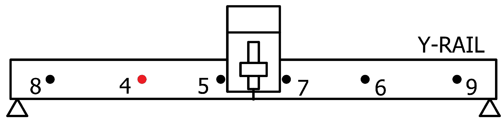
As can be inferred from
Figure 6 and
Figure 7, the tests for measuring the FRFs on the rails were taken in the worst possible scenario, the one in which the Y-rail and the cutting head are centered on Z-rail and Y-rail, respectively. There are three (3) measurement points on the Z-rail and six (6) on the Y-rail. The Y-rail has more points because it is more flexible, and its compliance is directly linked to vibrations of the tool. The red dot in
Figure 6 and
Figure 7 represents the excitation point that is fixed. Excitation direction is always perpendicular to the rail (X-axis). Measurement direction X is always perpendicular to the rail. The FRFs are calculated averaging the response of three hammer blows.
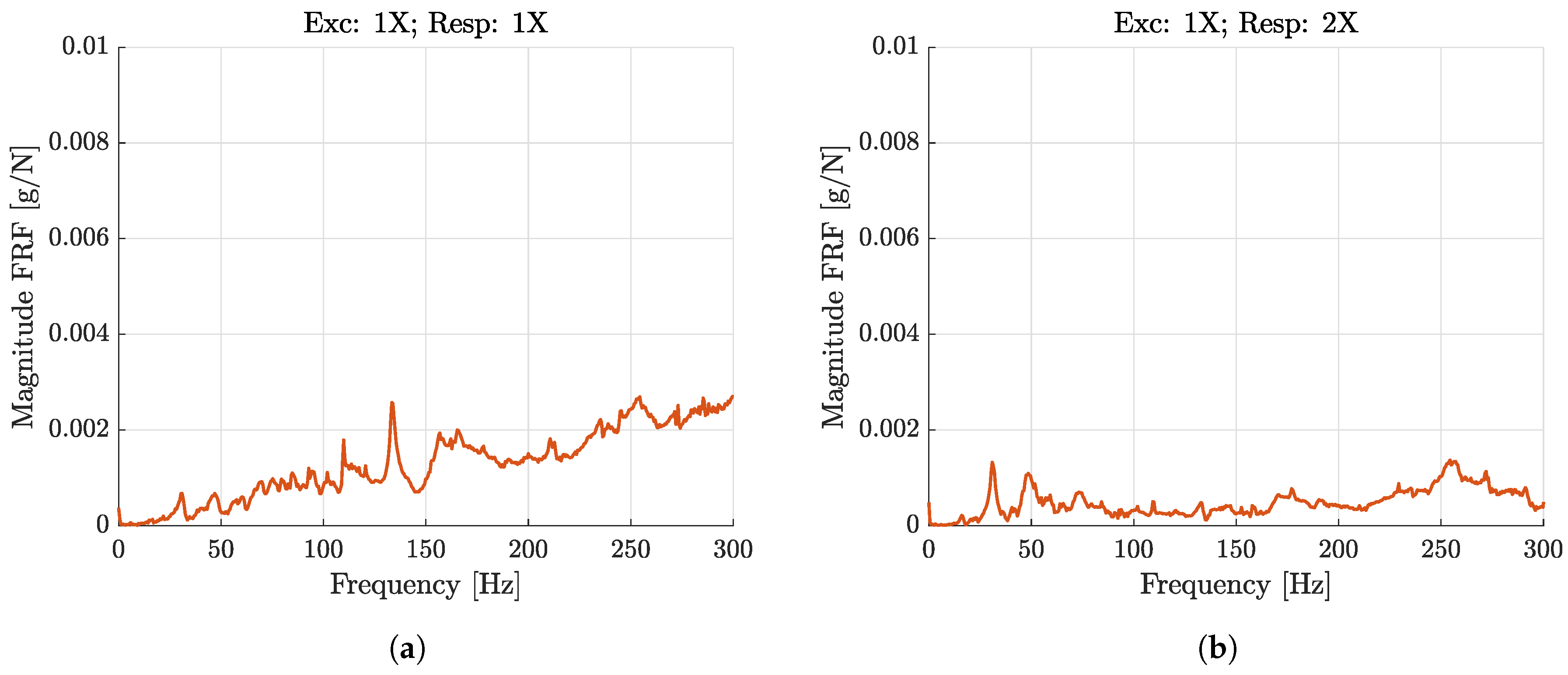
In
Figure 8a,b, the FRFs of Z-rail measured in two different points (1 and 2) caused by the excitation on point 1 are shown. In both FRFs, the first peaks occur at about 30 and 50 Hz, but they are much smaller, and amplitudes tend to increase at high frequency.
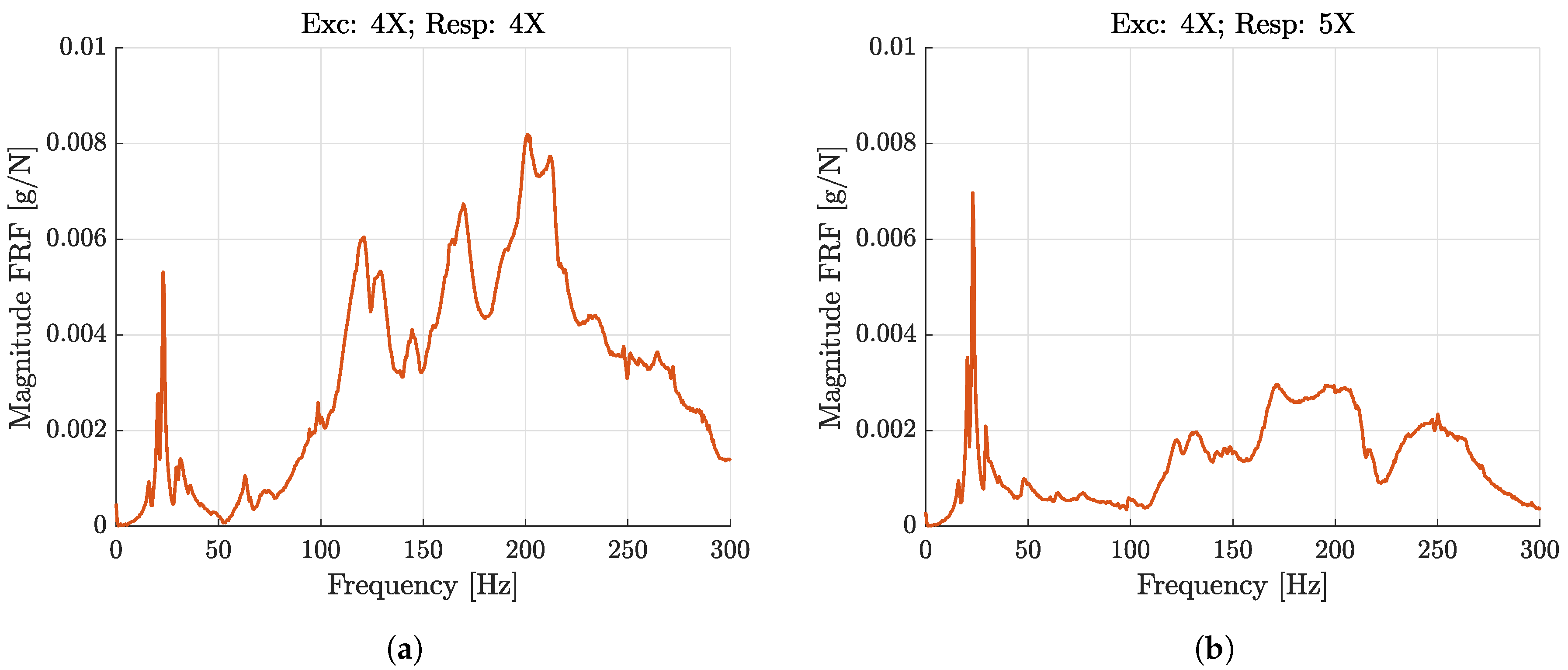
Considering Y-rail,
Figure 9a,b show an high peak at about 23 Hz, both in the direct and in the cross FRFs. Moreover, the magnitude is higher than the ones measured on Z-rail. It is important to notice the presence of some peaks around 200 Hz because, at this frequency, noisy vibrations appear.
In conclusion, it can be stated that Y-rail can have an important influence on the vibrations of the cutting head, whereas the contribution of Z-rail is very weak, confirming the hypothesis shown in the definition of the mathematical model in
Section 3.
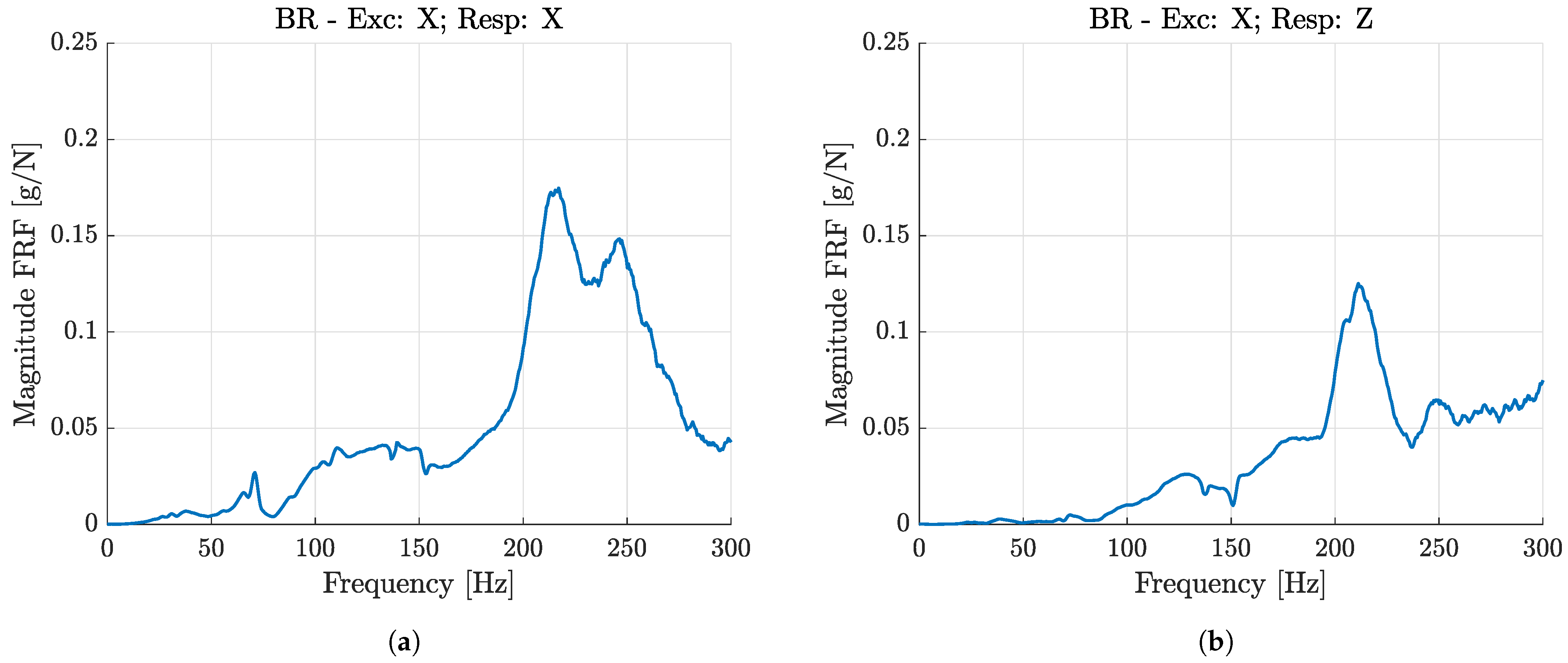
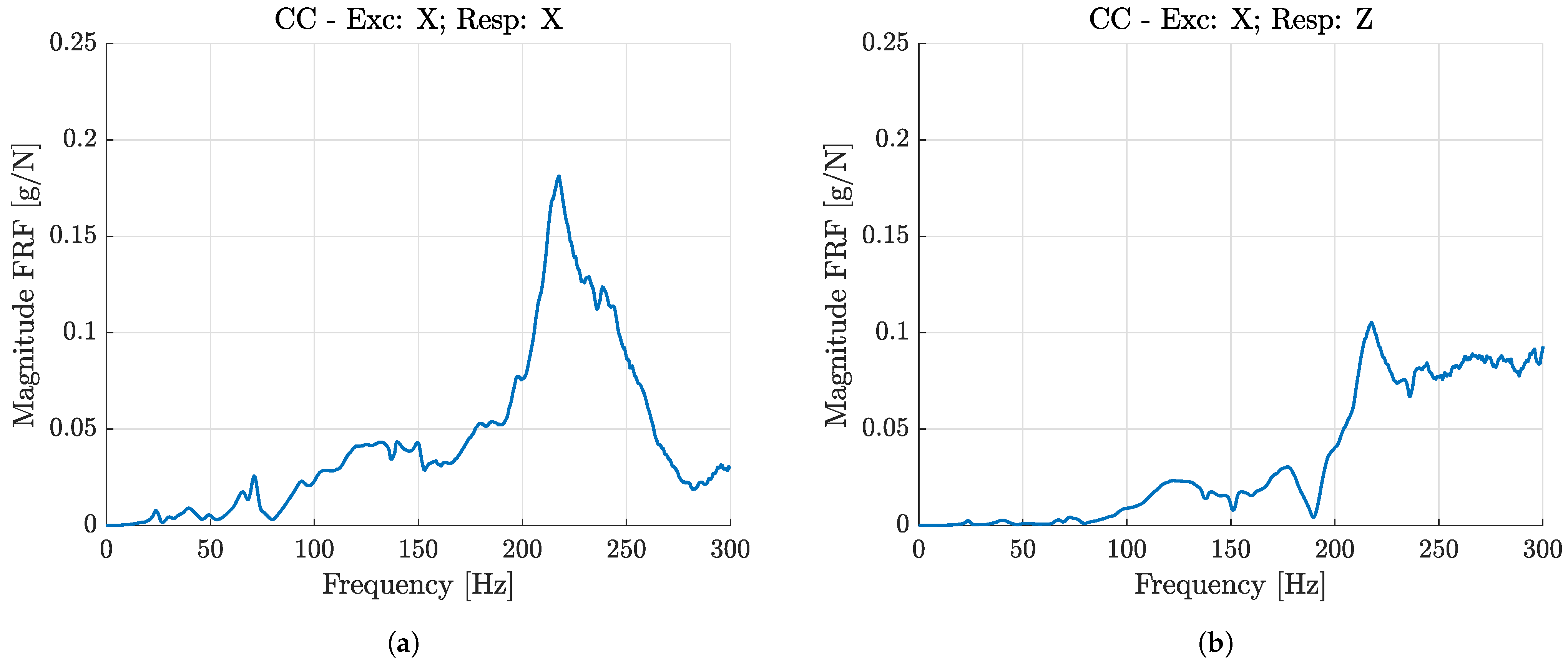
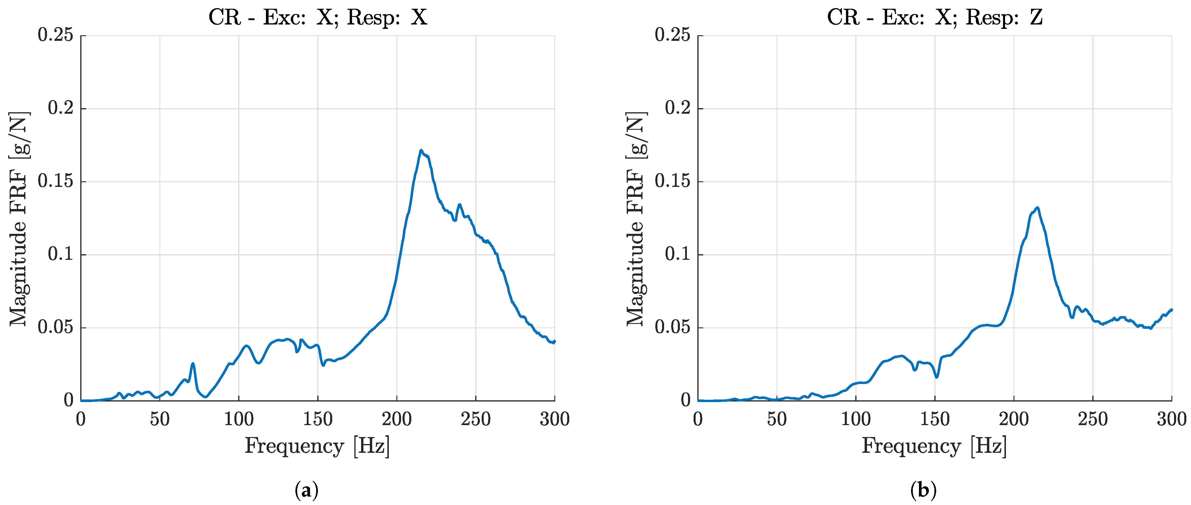
Considering the cutting head, the tests were performed hitting the tool along its vertical (X-axis) and measuring the response vertically (along the accelerometer X-axis) and radially (along the accelerometer Z-axis), following the scheme of
Figure 10.
The cutting head was then moved around the table and different tests were carried out. In
Figure 11, the testing positions of the cutting head are shown. The cutting head is displayed in the most central position that could be reached by the instrument without dismounting the conveyor belt. It is named the center-center (CC) position. The measured FRFs for some of the points are shown in
Figure 12,
Figure 13 and
Figure 14.
In agreement with the previous results [
18], the direct FRFs show the presence of two close resonance peaks in the range 200–300 Hz, the former with a frequency of 215 Hz, and the latter with a frequency of 248 Hz. The relative magnitude of the two peaks depends on the position of the cutting head in the Cartesian workspace. Cross FRFs show a resonance peak at 215 Hz.
5. Identification and Validation of the Mathematical Model
A best fitting process requires a first guess vector of design variables. The design variables of the equivalent robot model of
Figure 3 are:
,
,
,
,
,
,
,
,
, and
. First, guess values of these variables are found considering that two close resonance peaks are obtained when a main vibrating system with natural frequency
is coupled with an ancillary oscillator (AO) tuned to the same frequency. Analytical and experimental results show that the original resonance peak at
is substituted by two new resonance peaks, the former at lower frequency, and the latter at higher frequency [
22,
23]. The frequency interval between the two peaks depends on the ratio between the masses of the AO and of the main system (mass ratio). Since the masses and the stiffnesses are related through the natural frequency, the mass ratio can be transformed into a stiffness ratio. To obtain the first guess values of the design parameters, some further simplifications are made:
,
, and
. With the last assumptions, vertical vibrations depend on
, whereas longitudinal vibrations depend on
.
Since the identification is performed when the cutting head is in a corner of the workspace, where the rails reach the maximum stiffness, the motion of the Y-beam is neglected, and the equations of motion of the free undamped vibration of the equivalent robot become:
The terms of the mass matrix can be expressed as functions of the natural frequencies of the main system and of the AO, which are tuned to the same value
. The natural frequency of the main system is:
Hence, .
The natural frequency of the AO is:
Hence, .
The mass matrix of the coupled system becomes:
If stiffness
is expressed as a function of stiffness
:
the natural frequencies of the coupled system depend only on
and
and are given by these simple equations:
Therefore, looking at the measured FRF, it is possible to find the frequency of the minimum (
) between the close peaks and the frequency interval between them. The frequency of the minimum (230 Hz in the present case; see
Figure 12a) is used to define the tuning frequency
. Then, from Equation (
19), a value of
giving an interval between the resonance peaks of the system equal to the measured one can be found. The other first guess parameters are found, giving meaningful values to lengths and masses. Damping coefficients are calculated according to the following equation:
and assigning both to the main system and to the AO a damping ratio
.
The optimization algorithm uses the
fmincon function available in MATLAB. This function finds the scalar or the vector
X which minimizes the objective function FUN. In this case, the aim of the optimization is to determine the values of the design variables which minimize the difference between the measured FRFs, the direct FRF
and the cross one
, and the corresponding FRFs,
, and
, calculated by means of the mathematical model. Hence, the function FUN to be minimized is:
where
and
are two coefficients which adjust the influence of the FRFs, whereas
and
are two scale factors. The default algorithm
interior-point, a primal-dual method, was used to minimize the function FUN, and no further options were specified in the
fmincon function.
The
fmincon function starts the research of the optimum values of the parameters from the first guess values
of the design variables. The solution
X of the problem is found within the range defined by the lower (
) and upper (
) limit, that is:
No other constraints (linear and non-linear constraints) were specified in the fmincon function.
The calculation of the analytical FRFs is based on the 2 DOF model of the equivalent robotic system, and this implies that the measured FRFs used for the determination of the parameters of the model must be independent from the stiffness of the rails. Hence, the optimization algorithm is applied to the FRFs measured in the back-right (BR) position of the working table. The first guess values
of the design variables, defined through the approach described in the previous section, are summarized in
Table 1.
The values of the upper and lower limit of the values of the design variables are summarized in
Table 2.
The optimized values of the design variables, generated by means the
fmincon function assuming
,
,
, and
, are summarized in
Table 3.
Figure 15 compares the measured FRFs with the numerical FRFs that are obtained introducing the values of
Table 3 in the 2-DOF equivalent robotic model.
Figure 15 shows that the optimization algorithm leads to numerical FRFs which fit very well the measured FRFs. The resonance frequencies are matched, and the trends at the borders of the frequency range are also reproduced with high accuracy.
6. Effect of Cutting Head Position
Once defining the parameters of the equivalent robotic model, it is possible to develop the coupled model which accounts for rail dynamics.
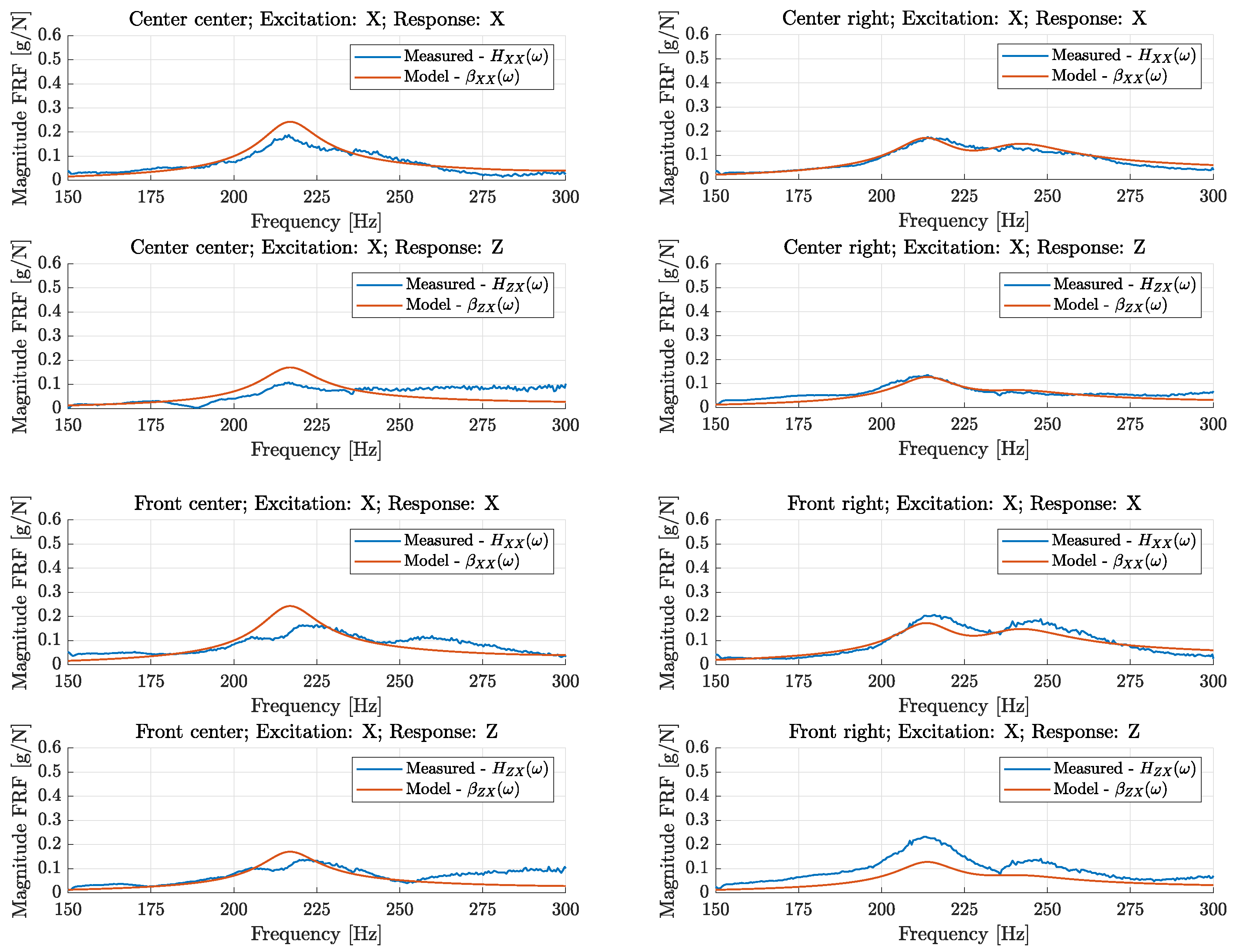
Figure 16 compares the measured FRFs in different positions of the working table with the FRFs predicted by the coupled model.
Figure 16 shows that the model fits the measured FRFs with good accuracy, and the mean modulus of the error of the model in the frequency range (150–300 Hz) is shown in
Table 4.
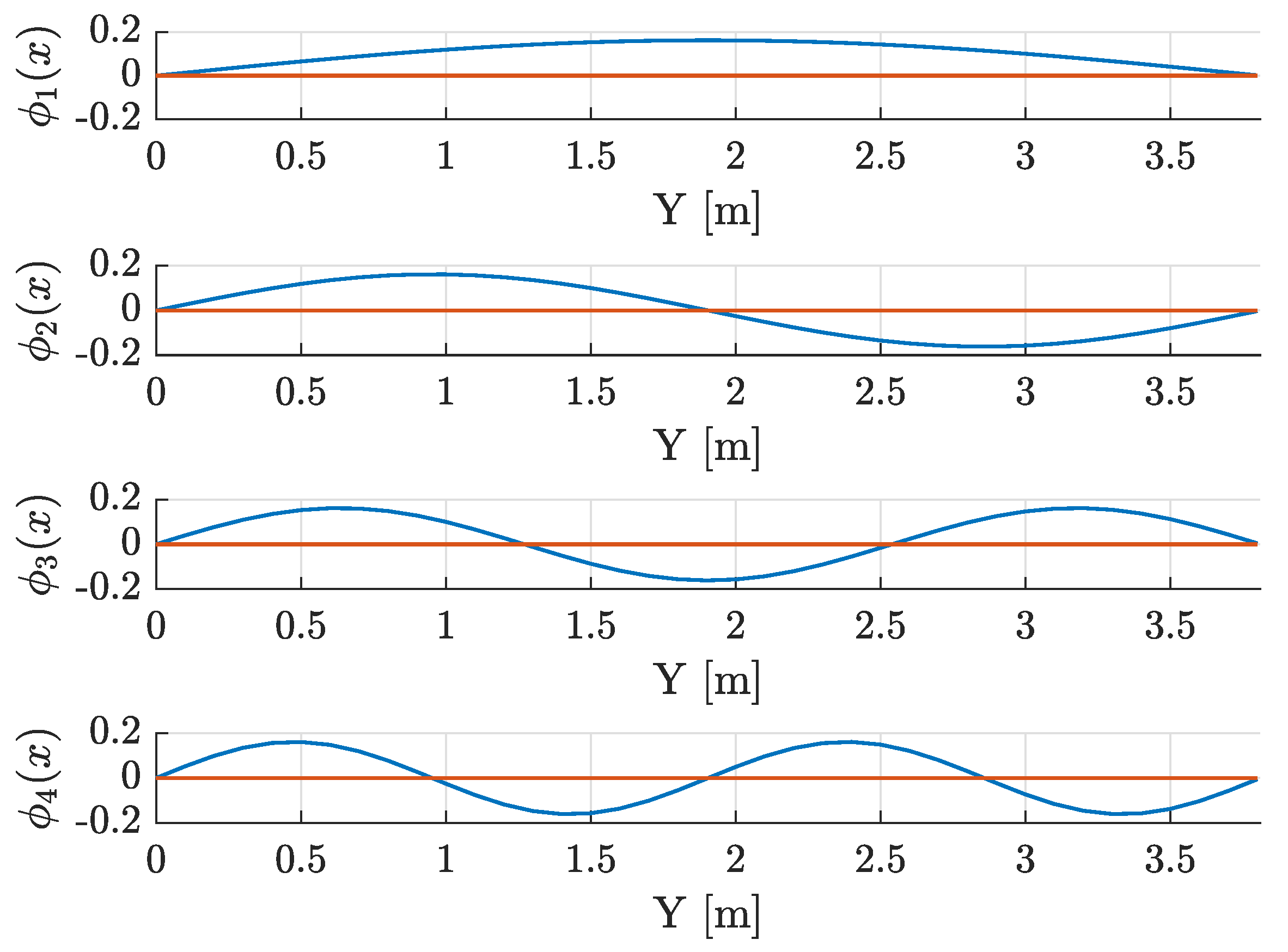
The FRFs change with the position of the cutting head along the Y-rail; hence, the dynamics of the rail have an important effect on the whole behavior of the system. The vibration of the cutting head excites different modes of the Y-rail, and the excited modes depend on the position of the head.
Figure 17 represents the first four vibration modes of the rail.
A mode of the rail is excited only if the cutting head is not located at a node of the mode. This means that the vibration of the cutting head will excite only the odds modes of the rail (1st and 3rd) when the cutting head is in the front-center (FC) or back-center (BC) position (see
Figure 11), since those positions correspond to the nodes of the even modes (2nd and 4th).
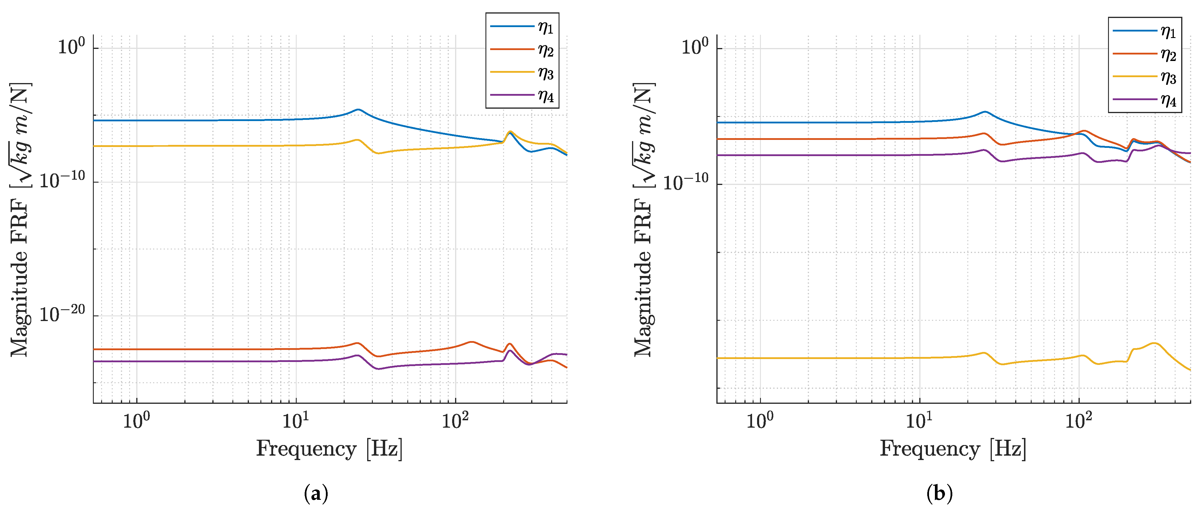
Figure 18a shows the FRFs between the
modal coordinate and the excitation force, when the cutting head is in the front-center (FC) position (or likewise in the back-center (BC) position), whereas
Figure 18b refers to the cutting head in the center-center (CC) position, which is approximately at
.
In
Figure 18a, the FRFs relative to the even modes are negligible, since these modes are not excited by the vibration of the cutting head which is located at the node of the mode. For the same reason, in
Figure 18b, the third mode is not excited and the corresponding FRF is negligible. This behavior can also be seen in the natural frequencies of the system.
Table 5 summarizes the natural frequencies of the Y-rail without the cutting head, whereas
Table 6 summarizes the natural frequencies of the coupled model, which considers the Y-rail and the cutting head, when the cutting head is in the front-center (FC) or back-center (BC) position and when it is in the center-center (CC) position.
Table 6 highlights that, when the cutting head is located at a node of a vibration mode of the Y-rail, the vibration mode of the Y-rail is not altered, and the natural frequency of that mode remains unchanged. Indeed, when the cutting head is in the CC position, which corresponds to a node of the third mode, only the natural frequency of the third mode remains unchanged.
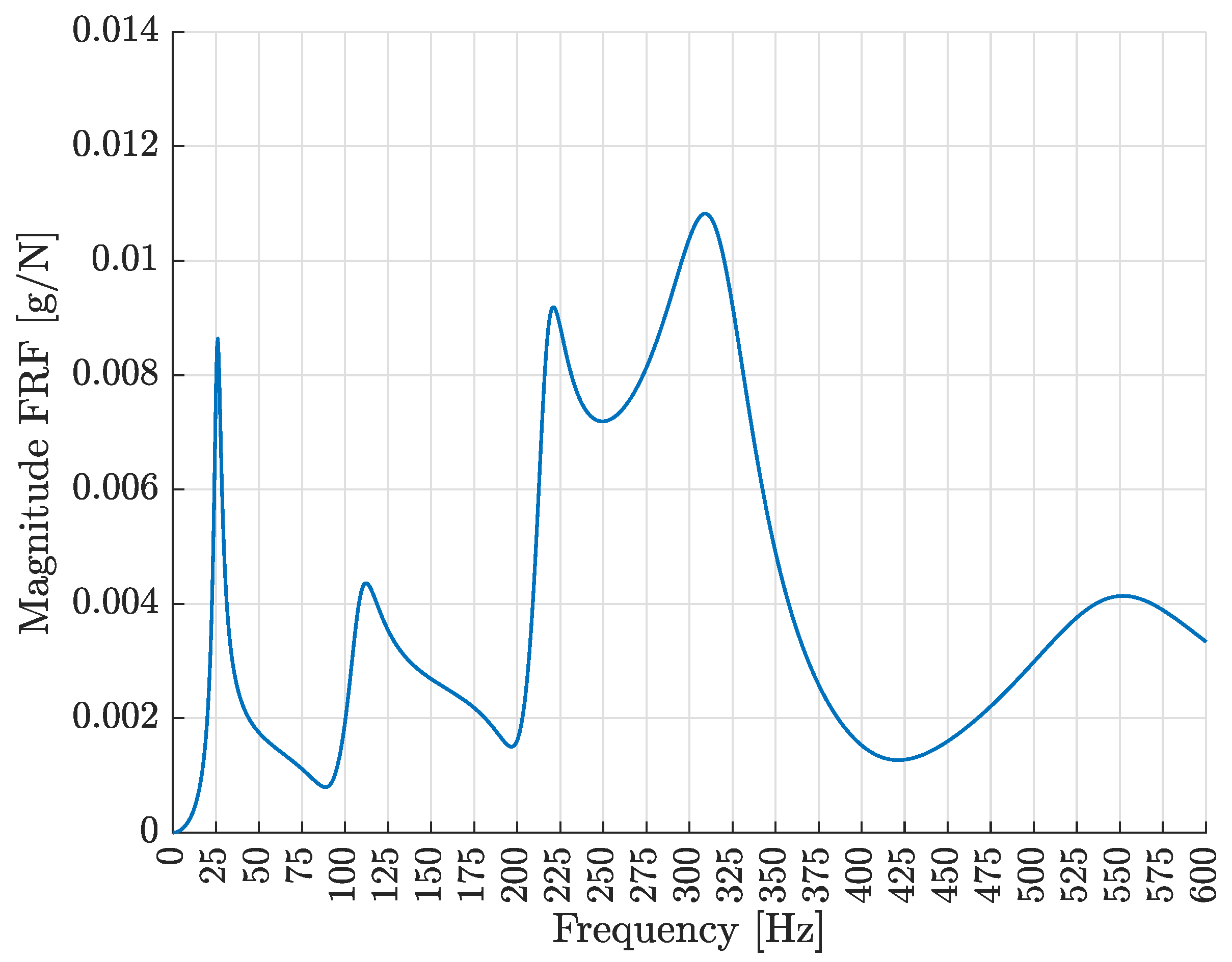
Figure 19 shows the FRF between the acceleration
and the cutting force in the X-direction, assuming the cutting head in center-center (CC) position.
The figure corroborates the previous results, since the first two peaks in the FRF are correlated with the first and second vibration mode of the Y-rail with the cutting head in CC position. The vibration mode relative to the third mode of the Y-rail is not excited; hence, it does not appear in the FRF. The third and fourth peaks in the FRF are related to the coupled dynamics between the Y-rail and the equivalent robotic arm, whereas the last peak is due to the fourth vibration mode of the Y-rail.
It is worth noting that the numerical FRF of
Figure 19 cannot be compared with the experimental FRF of
Figure 9, since, in numerical simulations, the exciting force is applied on the tool.
7. Example of Application of the Mathematical Model: Vibration Control by Means of a Dynamic Vibration Absorber
One of the possible applications of the proposed model is related to vibration control. In order to reduce the magnitude of the vibrations, structural modifications are usually made. When the excitation frequency is constant, such as in the present case, a typical structural modification is the introduction of a Tuned Vibration Absorber (TVA). This analysis can be performed using the Sherman-Morrison method [
24,
25], already shown in References [
18,
26], which makes it the calculation of the FRF of the modified system possible, starting from few FRFs of the original system and the dynamic stiffness of the lumped element
(the TVA). Therefore, starting from the FRFs of the proposed model, it is possible to simulate the effect of the TVA by means of simple calculations.
If the TVA is placed at the
coordinate, each element
of the receptance matrix can be modified as follows:
where
can be calculated as:
If the TVA is tuned at a specific frequency
, and mass
is as a fraction of the mass of the tool
M (usually around 0.05 ÷ 0.1
M), the stiffness of the TVA can be calculated from the natural frequency of the TVA:
Moreover, damping
can be calculated according to the damping ratio
of the material used for the TVA (for a steel beam, 0.01 ÷ 0.05):
As an example, a TVA installed on the cutting machine (specifically, on the tool), designed for controlling vibration in the X direction, is considered. Experimental tests and numerical simulations have shown how the FRF slightly changes when the cutting head moves along the rails; however, it is not possible to perform structural modifications on-the-fly, to account for such FRF changes. Therefore, the TVA has to be appropriately tuned to obtain good results in all the positions of the machine.
Using the FRF predicted by the mathematical model and the Sherman-Morrison method, a parametric analysis was carried out varying the tuning frequency in the range 210 ÷ 250 Hz and the damping ratio in the range 0.01 ÷ 0.05. The best results were found with the parameters listed in
Table 7.
Figure 20 shows that, both in the central position and in the lateral position, the TVA is able to minimize the amplitude of the FRF at the forcing frequency of the tool (217 Hz). The TVA introduces a peak at lower frequencies. This is a well-known behavior of TVAs that is not harmful in this case, since the excitation frequency is rather constant.
8. Conclusions
A model of the cutting machine is needed to control vibrations and noise in the whole workspace. The experimental test carried out with the modal analysis approach showed that: the fixed rails are very stiff, the moving rail has important resonances in the band of frequency of interest, and the cutting head has two important modes of vibration that can be excited by the pneumatic tool. The mathematical model of the cutting machine is composed of a modal model of the moving rail and of an equivalent robotic model of the cutting head, whose parameters are found by means of a best fitting method that uses only two measured FRFs. This model is able to predict the vibrations of the machine in various locations of the workspace and to assess the usefulness of vibration control strategies, such as the installation of a TVA in the tool. The increase in the number of measurement points in the cutting head does not appear very useful, since it could give more information about this vibrating system, but it would require long machine stop times, since many panels and accessories have to be removed to place the accelerometer on the structure of the cutting head. Conversely, the introduction of non-linear elements in the model appears more useful, since the tests showed some asymmetries (e.g., between the left and right side of the machine) that could be modeled only by a non-linear model.


