Article

Adaptive Obstacle Avoidance for a Class of Collaborative Robots

by
Giorgia Chiriatti
,
Giacomo Palmieri
*,
Cecilia Scoccia
,
Matteo Claudio Palpacelli
and
Massimo Callegari
Department of Industrial Engineering and Mathematical Sciences, Polytechnic University of Marche, 60131 Ancona, Italy
*
Author to whom correspondence should be addressed.
Machines 2021, 9(6), 113; https://doi.org/10.3390/machines9060113
Submission received: 6 May 2021 / Revised: 31 May 2021 / Accepted: 31 May 2021 / Published: 3 June 2021
(This article belongs to the Special Issue Collaborative Robotics and Adaptive Machines)

Abstract

:
In a human–robot collaboration scenario, operator safety is the main problem and must be guaranteed under all conditions. Collision avoidance control techniques are essential to improve operator safety and robot flexibility by preventing impacts that can occur between the robot and humans or with objects inadvertently left within the operational workspace. On this basis, collision avoidance algorithms for moving obstacles are presented in this paper: inspired by algorithms already developed by the authors for planar manipulators, algorithms are adapted for the 6-DOF collaborative manipulators by Universal Robots, and some new contributions are introduced. First, in this work, the safety region wrapping each link of the manipulator assumes a cylindrical shape whose radius varies according to the speed of the colliding obstacle, so that dynamical obstacles are avoided with increased safety regions in order to reduce the risk, whereas fixed obstacles allow us to use smaller safety regions, facilitating the motion of the robot. In addition, three different modalities for the collision avoidance control law are proposed, which differ in the type of motion admitted for the perturbation of the end-effector: the general mode allows for a 6-DOF perturbation, but restrictions can be imposed on the orientation part of the avoidance motion using 4-DOF or 3-DOF modes. In order to demonstrate the effectiveness of the control strategy, simulations with dynamic and fixed obstacles are presented and discussed. Simulations are also used to estimate the required computational effort in order to verify the transferability to a real system.

1. Introduction

As robot technology has advanced, new types of robots with improved safety functions have been developed. Nowadays, the trend toward collaborative robotics is growing as a consequence of more dynamic and flexible industrial scenarios. Collaborative robotics in the industrial systems allow robots and humans to share the workspace and interact to accomplish collaborative tasks; an overview of this trending topic can be found in [1,2]. From [3,4,5], it emerges that safety issues are central when the coexistence or collaboration between humans and robots is expected, which is increasing the need for standards and methods used to validate and certify the safety of a collaborative application before it can be installed at the industrial site. Moreover, since collaborative robotic systems should be configured to assist the operator during their work, they are often equipped with sensor systems able to perceive the human motion and to detect the position of objects inside the workspace that may generate a risk of collision with the manipulator. Simple 2D cameras can be used for detecting [6] and predicting [7] the motion of the human arm on a working surface, or to calibrate the user-frame of the robot [8]. Vision systems able to generate depth space images are typically used to perceive the human pose in the 3D space [9,10,11]; data from such sensors can be easily elaborated to extrapolate the coordinates of skeleton models replicating the human motion [12,13]. Other types of optical sensors can be used, e.g., eye tracking systems able to detect the points of the screen on which the human is focusing its sight, translating such information into a command for the robot [14].
In addition to dedicated hardware and design principles, collaborative robotics implies specific control strategies, such as collision avoidance control techniques for dynamically varying environments: once fixed or moving obstacles are detected inside the workspace, the control must be able to modify in real-time the motion of the robot in order to avoid impacts at any point of its kinematic chain. Fixed obstacles can be thought of as objects inadvertently left inside the workspace, such as furniture elements or mechanical tools, whereas dynamic moving obstacles may represent humans operating in the shared workspace.
Several methods are available in the literature for collision avoidance; a common approach exploits the same principles of the artificial potential fields method, typically used for the path planning of mobile robots [15,16,17]: a potential field can be associated with each obstacle, so that a repulsive velocity inversely proportional to the distance from that obstacle is assigned to the control points along the kinematic chain of the manipulator. Thus, in addition to the motion imposed to the end-effector, a repulsive velocity vector can be applied to the point of the robot that is closer to one of the obstacles, adding a task to the control system [18,19,20,21,22,23,24,25]. This kind of approach was studied by the authors in [26,27] for a planar case; in addition to the standard method, a modified repulsive velocity method was introduced, which depended on the velocity, in addition to the position, of the obstacle, improving the capability of the algorithm to compensate for moving obstacles. Starting from this stage of the research, the present paper adapts the collision avoidance algorithms to a class of 6-DOF industrial manipulators, i.e., the Universal Robots collaborative robots family [28]. Furthermore, some significant new contributions are introduced:
  • While in previous works the safety regions enveloping the structure of the robot were defined as spheres centred on a series of control points equally spaced along the serial kinematic chain, a more efficient strategy is proposed here defining only one safety volume for each link; such volume is the combination of a cylinder, with a height equal to the length of the link, and two hemispheres at the extremities of the link.
  • In order to adapt the algorithm to different cases, with fixed or moving obstacles, the radius of the cylindrical/hemispherical safety volume of each link is variable, as a function of the obstacle velocity: a small radius is adopted for fixed obstacles, facilitating the mobility of the robot, whereas the radius increases with the speed of the obstacle, so that the risk of collision is reduced for the dynamic case.
  • Three different modalities for the collision avoidance control law are proposed, which differ in the type of motion admitted for the perturbation of the end-effector. The first mode, the most general, allows for a 6-DOF perturbation of the end-effector, whose pose may vary in position and orientation in order to avoid a collision. If such condition is not admissible due to the specific application, some restrictions can be imposed. As an example, in this paper, two additional modes characterized by a reduced mobility of the perturbation are proposed. The second mode allows for a 4-DOF Schoenflies-like perturbation, where all translations and the rotation about the vertical axis are admitted. If the last rotation is not admitted, the third mode can be used, where the orientation of the end-effector remains unchanged during the perturbation due to a collision avoidance.
Details on the abovementioned formulation of the control law and the implementation of the three modalities are given in Section 2. Section 3 presents a series of simulations performed in order to test the algorithms and to verify the transferability to a real system, in terms of computational time. Results and insights on future works are then discussed in the conclusion (Section 4).

2. Motion Control Law
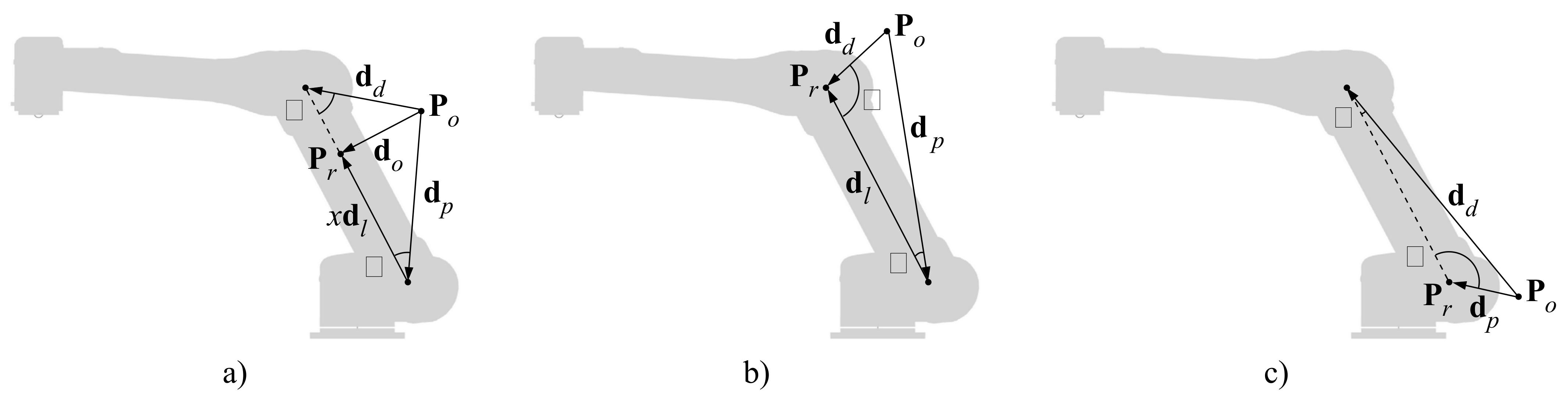
Starting from results obtained in previous studies [26], in this paper, the algorithms for collision avoidance are extended and implemented for Universal Robots manipulators; the UR5 robot is used as test case, but the implementation to other UR manipulators is straightforward due to the identical kinematic structure, except for the lengths of the links. The kinematic chain, characterized by eight control points ( A , B , C , C 1 , D , E , F , G ), is shown in Figure 1, whereas Table 1 summarizes the dimensions of the links. The 6-DOF mobility is conferred by all revolute joints: the base ( θ 1 ), the shoulder ( θ 2 ), the elbow ( θ 3 ) and three wrist joints ( θ 4 , θ 5 , θ 6 ). They are the components of the joint space position vector: q = [ θ 1 θ 2 θ 3 θ 4 θ 5 θ 6 ] T . In the Cartesian space, according to the Euler angle ZYZ convention, the pose of the end-effector is defined by x = [ x y z α β γ ] T . The forward kinematics of the manipulator are described by:
x = f ( q )
x ˙ = x ˙ p ω = J p J o q ˙ = J ( q ) q ˙
where f is the expression of the position forward kinematics; x ˙ is the velocity vector composed by the linear velocity vector x ˙ p and the angular velocity ω ; J is the ( 6 × 6 ) analytic Jacobian matrix, composed by J p and J o , which are the ( 3 × 6 ) position and orientation Jacobian matrices, respectively. The inverse velocity problem can be solved by:
q ˙ = J ( q ) 1 x ˙
Nevertheless, a damped least-square strategy [29] is adopted to prevent singularity problems which appear when the manipulator is close to a singular configuration. According to [30], the damped inverse matrix can be obtained as:
J * = J T ( JJ T + λ 2 I ) 1
where λ is the damping factor, modulated as a function of the smaller singular value of the Jacobian matrix. In particular, if the smallest singular value σ m i n is higher than a predefined threshold ϵ , then the damped inverse law coincides with the standard inversion ( λ = 0 ) ; otherwise, if σ m i n < ϵ , then the value of λ increases inversely to σ m i n up to a maximum value of λ m a x .
Thus, knowing the initial joint position q 0 , the joint position law can be obtained by a discrete integration in time domain:
q ( t + d t ) = q 0 ( t ) + q ˙ ( t ) d t q ˙ = J * x ˙
In order to define an obstacle avoidance control strategy, it is necessary to detect the link of the manipulator with the highest risk of collision with the obstacles inside of the workspace. Thus, it is necessary to calculate the distance of each obstacle from each link, in order to detect the obstacle–link pair characterized by the minimum distance. Eight segments, delimited by the control points represented in Figure 1, are considered in this algorithm. The distance of an obstacle P O from a link [20,31] is calculated according to the schemes of Figure 2, where d l is the vector connecting the proximal to the distal extremity of the link; d p and d d are the distances between the obstacle and the proximal and distal extremities of the link, respectively; P r is the point of the link closest to the obstacle. In detail:
(a)
If cos α 0 and cos β 0 , then the distance d o = P r P o is orthogonal to the link, and the position of P r along the link is defined by the scalar parameter x:
d o = | d l × d p | d l x = d p cos α d l , 0 < x < 1
(b)
If cos β < 0 , then the point P r is coincident with the distal extremity of the link, thus:
d o = d d x = 1
(c)
If cos α < 0 , then the point P r is coincident with the proximal extremity of the link, thus:
d o = d p x = 0
Figure 3 shows a condition conforming to the case (a). The obstacle influences the motion of the robot if the distance d o is lower than the radius r, which is a tunable parameter of the algorithm. Thus, the region of interest of each link can be visualized as a cylinder with two hemispheres at its extremities, all of radius r. The repulsive velocity x ˙ 0 is applied to P r , whose position is known from one of Equations (6)–(8). Only one of the links of the manipulator will be subjected to the repulsive velocity, i.e., the one which is closest to one of the obstacles.
The choice of a proper value for r is a critical issue for the tuning of the algorithm. A small radius leads to reduced regions of influence, with a limitation of the cases where an obstacle may interfere with the robot; on the other hand, for quickly moving obstacles, the required readiness of the anti-collision control may be too demanding for standard controllers. Thus, a larger radius is desirable for moving obstacles, whereas fixed obstacles can also be avoided with small regions of influence. Consequently, the strategy adopted in this work is to vary r according to the ramp plotted in Figure 4a, as a function of the velocity v o of the obstacle closest to the link [31]. A possible alternative could be to consider the relative speed between the obstacle and the robot instead of v o , which takes into account different scenarios, such as a fixed manipulator with moving obstacles and vice versa, or obstacles and robots both in motion.
The control strategy used for the collision avoidance is based on an additional velocity task assigned the point P r of the robot, in addition to the velocity imposed on the end-effector in order to execute the planned trajectory. Three different modalities are described in detail in the following subsections.

2.1. Mode I: 6-DOF Perturbation

The control law is based on a Closed-Loop Inverse Kinematics (CLIK) approach, with two velocity tasks imposed on the manipulator. The first task assigns the velocity x ˙ e to the end effector, by means of the analytic Jacobian J :
J q ˙ = x ˙ e J p J o q ˙ = x ˙ e p ω
The second task imposes the translation velocity x ˙ 0 assigned to the point P r of the kinematic chain in order to avoid the collision; in this case, only the upper ( 3 × 6 ) part of the Jacobian J 0 associated with the linear velocity of P r is used:
J 0 = J 0 p J 0 o J 0 p q ˙ = x ˙ 0
The damped least square algorithm is applied to invert J and J 0 p , guaranteeing numerical stability even in proximity to singular configurations. Thus, the combinations of the velocity tasks expressed in Equations (9) and (10) give
q ˙ = J * x ˙ e + K e + J 0 p * a v v r e p d ^ o
where:
  • K is a positive-defined gain matrix, for simplicity set as K = k e I .
  • The position error e between the desired x e and actual position x is defined as [30]:
    e = e p e o = p e p 1 2 n × n e + s × s e + a × a e
    where e p is the translation error vector and e o is the orientation error vector; the position and orientation of the end-effector are, respectively, expressed by the vector p and the rotation matrix R = [ n s a ] , with n , s , a being the unit vectors of the end-effector frame.
  • The repulsive velocity x ˙ 0 is modulated as x ˙ 0 = a v v r e p d ^ o , where v r e p is a tunable magnitude and a v is an activation factor that is function of the distance d o (Figure 4b) according to
    a v = 1 d o r m i n d o r r m i n r 2 r m i n < d o < r 0 d o r
The first term of Equation (11) ensures the planned velocity of the end-effector with a minimum effort in terms of joints speeds; when there is a risk of collision, the second term is activated, generating a 6-DOF perturbation of the end-effector motion. The error is then compensated by the proportional corrective term when the risk of collision is exceeded.

2.2. Mode II: 4-DOF Schoenflies Perturbation

A 6-DOF perturbation of the end-effector motion, as in the previous case, could be unacceptable in some conditions, for example, if the orientation of the tool cannot vary during its manipulation. In this case, only a 4-DOF perturbation of the Schoenflies type is admitted. Thus, positioning errors due to translations along the three axes and a rotation about the vertical axis z are allowed. The control law is modified as follows:
q ˙ = J * x ˙ e + K e + J I I * a v v r e p d ^ o 0 2 × 1
The Jacobian matrix of the mode II, of dimension ( 5 × 6 ) , is defined as:
J I I = J 0 p j o 4 j o 5
where J 0 p is the translation part of the Jacobian associated with P r , whereas j o 4 and j o 5 are the fourth and fifth rows of the orientation Jacobian matrix J o of the end-effector, respectively. In this way, the second task assigns to P r the velocity required to avoid the collision, imposing at the same time null angular velocity components along x and y axes for the consequent perturbation motion of the end-effector.

2.3. Mode III: Perturbation with Fixed Orientation

In this last case, a further restriction is given to the type of motion allowed for the end-effector perturbation: only translations are admitted, whereas the orientation must remain unchanged during the motion. Similarly to the previous case, it is:
q ˙ = J * x ˙ e + K e + J I I I * a v v r e p d ^ o 0 3 × 1
Now, the Jacobian matrix of the second term has a ( 6 × 6 ) dimension; it is composed by the translation part of J 0 and the orientation part of J :
J I I I = J 0 p J o
Thus, a null angular velocity is imposed on the perturbation term of the control law.

3. Simulations

Algorithms were tested in Matlab in a series of simulations using in all cases a common set of parameters, summarized in Table 2. A limit θ ˙ m a x of the angular velocity was imposed to all the joints as a saturation threshold, in order to avoid high speeds at joints that may occur when a collision avoidance task is planned in the Cartesian space.
The error due to saturation was subsequently recovered by the proportional corrective term of the control law.
In the first three examples, illustrated in Figure 5, Figure 6 and Figure 7, the robot holds in a fixed position, whereas a moving obstacle will interfere with its end-effector. Such obstacle has a linear velocity of 0.25 m/s along the y direction. Six steps of the motion are plotted, from 0 to T = 2 s ; when the obstacle reaches the region of influence of the end effector ( t 0.6 s ) , the radius of the safety region increases, due to the speed of the obstacle, and the robot starts to react to keep the obstacle outside that area.
In the first example (Figure 5), the robot avoids the obstacle with the mode I, thus with a 6-DOF perturbation of the end-effector pose. In the second example (Figure 6) the control law is in mode II, thus the robot reacts with a 3-DOF translation and a rotation about z, as clearly visible at t = 1.3 s , whereas the other angular velocity components are constantly zero. The example in Figure 7 refers to the mode III: the manipulator avoids the obstacle, maintaining the orientation of the end-effector.
The profiles of joints rotations and speeds related to the abovementioned examples are plotted in Figure 8, Figure 9 and Figure 10. In all cases, the saturation of joint speed is reached for at least one motor. Moreover, mode I (Figure 8) provides a response where all motors are quite uniformly recruited for the anti-collision task; transitioning into mode II and III, the role of motors 4 and 5 is reduced.
In order to compare the effort required of the motors in the three different modes, the norm of the joints angular velocity vector | | q ˙ | | and the norm of the joints angular acceleration vector | | q ¨ | | were analyzed, and their maximum values assumed during the motion, | | q ˙ | | m a x and | | q ¨ | | m a x , respectively, were used as indexes. Table 3 shows the results of the simulations: the three modes are equivalent in terms of maximum acceleration; however, the length of the path is slightly lower for mode I, with a consequent higher value of maximum joint speed. The three modes are also substantially equivalent in terms of computational time, referring to the time required to compute a single iteration of the control loop. A further comparison of the modes should be conducted considering different metrics, such as the power consumption or torque peaks; thus, a dynamical modeling of the robot in order to find an optimal solution will be the object of future work.
Finally, an example of obstacle avoidance in mode I is given in Figure 11 considering the following scenario: the robot moves on a linear path, while three obstacles will interfere; two of them are fixed, and the other moves along x at a speed of 0.1 m / s . The first obstacle encountered will collide with the end-effector at approximately t = 1.6 s ; due to the obstacle speed, the radius of the region of interest is increased, reducing the risk of collision. At t 2.8 s , the effect of the second obstacle is visible: the radius r is smaller in this case, being the fixed obstacle. The third obstacle, also fixed, is reached at t 3.2 s ; its effect is to push downwards on the 5th link of the manipulator, generating an error in the trajectory of the end-effector that is suddenly recovered to reach the correct final position at t = 5 s .
For this example, a quantitative comparison is also presented between the three different control modalities (the trajectories obtained with modes II and III are not reported for the sake of brevity, but are visible on the videos provided as Supplementary Material). Table 4 shows that in this case, modes II and III give the shortest path, whereas mode II is also the most advantageous in terms of maximum speed. There are no differences for the accelerations, as for the computational times, which are very similar. In summary, considering the results collected in Table 3 and Table 4, the three modes are very similar in terms of motor effort. Therefore, the control mode must be selected according to the application: if, for example, a potentially dangerous instrument is moved, it may be advisable to maintain it in a fixed orientation, avoiding potential collisions or exposures to the face of the collaborating human. On the other hand, if the orientation of the end-effector is not a critical issue, the control mode I can be selected to increase the ability to avoid collisions; in fact, the greater number of degrees of freedom available to create repulsive motions helps in general to avoid obstacles.
In addition to verifying the correctness of the method, the simulations presented in this section also have the purpose of evaluating the computational effort required to implement the related algorithms in a real system. In this regard, the final objective of this research is to transfer the control framework to a real system, now under construction in laboratory, where the robot will be equipped with a vision system composed by multiple 3D cameras, able to acquire the surrounding environment and extrapolate the position of objects and humans within the workspace. Fixed obstacles simulated in this study can be thought of as fixed objects inadvertently left inside the workspace, such as furniture elements or mechanical tools, whereas dynamic moving obstacles may represent humans operating in the shared workspace.
In the implementation in a real system, the speed of execution of the control loop is expected to be a critical issue. Based on the results presented in this paper, it can be summarized that the on-line motion control is able to run with a cycle time of approximately 10 3 s , lower than rates typically used in the communication between external controllers and the main controllers of robots. Furthermore, a standard laptop (i7 CPU @1.8 GHz, 16 GB RAM) was used for simulations; thus, a reduction in computational times can be expected if a higher performing hardware is used.

4. Conclusions

In this document, an obstacle avoidance strategy for UR manipulators moving in dynamically variable environments is presented and verified by simulation. Starting from algorithms already developed by the authors, some new contributions are introduced, such as the cylindrical shape of the regions of influence that wraps the kinematic chain of the manipulator with a variable radius according to the speed of the obstacle in collision. In addition, three different ways to avoid collisions are proposed, which differ in the type of movement allowed for the perturbation of the end-effector.
In addition to to confirming the effectiveness of the control strategy, the simulations provide an estimate of the computational effort required to run the algorithms, which is in line with the typical requirements of robot controllers and can be improved by using higher performing hardware.
Future work will involve extending the algorithms to 7-DOF redundant manipulators, where the robot’s additional degree of freedom can be exploited to further increase collision avoidance.
Furthermore, the implementation in real systems is currently under development, and preliminary tests confirm the validity of the proposed control strategy.

Supplementary Materials

Supplementary materials are available at https://www.mdpi.com/article/10.3390/machines9060113/s1.

Author Contributions

Conceptualization, G.P., G.C. and C.S.; investigation, G.P., G.C. and C.S.; writing—original draft preparation, G.C.; writing—review and editing, G.P.; supervision, G.P., M.C.P. and M.C. All authors have read and agreed to the published version of the manuscript.

Funding

This work was partly funded by the project URRA, “Usability of robots and reconfigurability of processes: enabling technologies and use cases”, on the topics of User-Centered Manufacturing and Industry 4.0, which is part of the project EU ERDF, POR MARCHE Region FESR 2014/2020–AXIS 1–Specific Objective 2–ACTION 2.1, “HD3Flab-Human Digital Flexible Factory of the Future Laboratory”, coordinated by the Polytechnic University of Marche.

Institutional Review Board Statement

Not applicable.

Informed Consent Statement

Not applicable.

Conflicts of Interest

The authors declare no conflict of interest.

References

  1. Vicentini, F. Collaborative robotics: A survey. J. Mech. Des. 2021, 143, 040802. [Google Scholar] [CrossRef]
  2. El Zaatari, S.; Marei, M.; Li, W.; Usman, Z. Cobot programming for collaborative industrial tasks: An overview. Robot. Auton. Syst. 2019, 116, 162–180. [Google Scholar] [CrossRef]
  3. Lasota, P.A.; Fong, T.; Shah, J.A. A Survey of Methods for Safe Human-Robot Interaction; Now Publishers: Hanover, MA, USA, 2017. [Google Scholar]
  4. Robla-Gómez, S.; Becerra, V.M.; Llata, J.R.; González-Sarabia, E.; Torre-Ferrero, C.; Pérez-Oria, J. Working Together: A Review on Safe Human-Robot Collaboration in Industrial Environments. IEEE Access 2017, 5, 26754–26773. [Google Scholar] [CrossRef]
  5. Valori, M.; Scibilia, A.; Fassi, I.; Saenz, J.; Behrens, R.; Herbster, S.; Bidard, C.; Lucet, E.; Magisson, A.; Schaake, L.; et al. Validating Safety in Human–Robot Collaboration: Standards and New Perspectives. Robotics 2021, 10, 65. [Google Scholar] [CrossRef]
  6. Morlock, M.; Bajrami, V.; Seifried, R. Trajectory tracking with collision avoidance for a parallel robot with flexible links. Control Eng. Pract. 2021, 111, 104788. [Google Scholar] [CrossRef]
  7. Dinh, K.H.; Oguz, O.; Huber, G.; Gabler, V.; Wollherr, D. An approach to integrate human motion prediction into local obstacle avoidance in close human-robot collaboration. In Proceedings of the 2015 IEEE International Workshop on Advanced Robotics and its Social Impacts (ARSO), Lyon, France, 30 June–2 July 2015; pp. 1–6. [Google Scholar]
  8. Pagani, R.; Nuzzi, C.; Ghidelli, M.; Borboni, A.; Lancini, M.; Legnani, G. Cobot User Frame Calibration: Evaluation and Comparison between Positioning Repeatability Performances Achieved by Traditional and Vision-Based Methods. Robotics 2021, 10, 45. [Google Scholar] [CrossRef]
  9. Flacco, F.; Kröger, T.; De Luca, A.; Khatib, O. A depth space approach to human-robot collision avoidance. In Proceedings of the 2012 IEEE International Conference on Robotics and Automation, Saint Paul, MN, USA, 14–18 May 2012; pp. 338–345. [Google Scholar]
  10. Schmidt, B.; Wang, L. Depth camera based collision avoidance via active robot control. J. Manuf. Syst. 2014, 33, 711–718. [Google Scholar] [CrossRef]
  11. Mohammed, A.; Schmidt, B.; Wang, L. Active collision avoidance for human–robot collaboration driven by vision sensors. Int. J. Comput. Integr. Manuf. 2017, 30, 970–980. [Google Scholar] [CrossRef]
  12. Du, G.; Long, S.; Li, F.; Huang, X. Active Collision Avoidance for Human-Robot Interaction With UKF, Expert System, and Artificial Potential Field Method. Front. Robot. AI 2018, 5, 125. [Google Scholar] [CrossRef] [PubMed]
  13. Scimmi, L.S.; Melchiorre, M.; Troise, M.; Mauro, S.; Pastorelli, S. A Practical and Effective Layout for a Safe Human-Robot Collaborative Assembly Task. Appl. Sci. 2021, 11, 1763. [Google Scholar] [CrossRef]
  14. Scalera, L.; Seriani, S.; Gallina, P.; Lentini, M.; Gasparetto, A. Human–Robot Interaction through Eye Tracking for Artistic Drawing. Robotics 2021, 10, 54. [Google Scholar] [CrossRef]
  15. Gasparetto, A.; Boscariol, P.; Lanzutti, A.; Vidoni, R. Path planning and trajectory planning algorithms: A general overview. In Motion and Operation Planning of Robotic Systems; Springer: Berlin/Heidelberg, Germany, 2015; pp. 3–27. [Google Scholar]
  16. Xu, X.; Hu, Y.; Zhai, J.; Li, L.; Guo, P. A novel non-collision trajectory planning algorithm based on velocity potential field for robotic manipulator. Int. J. Adv. Robot. Syst. 2018, 15, 1729881418787075. [Google Scholar] [CrossRef] [Green Version]
  17. Wang, W.; Zhu, M.; Wang, X.; He, S.; He, J.; Xu, Z. An improved artificial potential field method of trajectory planning and obstacle avoidance for redundant manipulators. Int. J. Adv. Robot. Syst. 2018, 15. [Google Scholar] [CrossRef] [Green Version]
  18. Zhang, H.; Jin, H.; Liu, Z.; Liu, Y.; Zhu, Y.; Zhao, J. Real-time kinematic control for redundant manipulators in a time-varying environment: Multiple-dynamic obstacle avoidance and fast tracking of a moving object. IEEE Trans. Ind. Inform. 2019, 16, 28–41. [Google Scholar] [CrossRef]
  19. Safeea, M.; Neto, P.; Bearee, R. On-line collision avoidance for collaborative robot manipulators by adjusting off-line generated paths: An industrial use case. Robot. Auton. Syst. 2019, 119, 278–288. [Google Scholar] [CrossRef] [Green Version]
  20. Khatib, O. Real-Time Obstacle Avoidance for Manipulators and Mobile Robots. Int. J. Robot. Res. 1986, 5, 90–98. [Google Scholar] [CrossRef]
  21. Maciejewski, A.A.; Klein, C.A. Obstacle Avoidance for Kinematically Redundant Manipulators in Dynamically Varying Environments. Int. J. Robot. Res. 1985, 4, 109–117. [Google Scholar] [CrossRef] [Green Version]
  22. Abhishek, T.S.; Schilberg, D.; Doss, A.S.A. Obstacle Avoidance Algorithms: A Review. In IOP Conference Series: Materials Science and Engineering; IOP Publishing: Bristol, UK, 2021; Volume 1012, p. 012052. [Google Scholar]
  23. Perdereau, V.; Passi, C.; Drouin, M. Real-time control of redundant robotic manipulators for mobile obstacle avoidance. Robot. Auton. Syst. 2002, 41, 41–59. [Google Scholar] [CrossRef]
  24. Moe, S.; Pettersen, K.Y.; Gravdahl, J.T. Set-based collision avoidance applications to robotic systems. Mechatronics 2020, 69, 102399. [Google Scholar] [CrossRef]
  25. Zhang, W.; Cheng, H.; Hao, L.; Li, X.; Liu, M.; Gao, X. An obstacle avoidance algorithm for robot manipulators based on decision-making force. Robot. Comput. Integr. Manuf. 2021, 71, 102114. [Google Scholar] [CrossRef]
  26. Scoccia, C.; Palmieri, G.; Palpacelli, M.C.; Callegari, M. A Collision Avoidance Strategy for Redundant Manipulators in Dynamically Variable Environments: On-Line Perturbations of Off-Line Generated Trajectories. Machines 2021, 9, 30. [Google Scholar] [CrossRef]
  27. Scoccia, C.; Palmieri, G.; Palpacelli, M.; Callegari, M. Real-Time Strategy for Obstacle Avoidance in Redundant Manipulators. Mech. Mach. Sci. 2021, 91, 278–285. [Google Scholar]
  28. Kebria, P.M.; Al-Wais, S.; Abdi, H.; Nahavandi, S. Kinematic and dynamic modelling of UR5 manipulator. In Proceedings of the 2016 IEEE International Conference on Systems, Man, and Cybernetics (SMC), Budapest, Hungary, 9–12 October 2016; pp. 004229–004234. [Google Scholar]
  29. Moe, S.; Antonelli, G.; Teel, A.R.; Pettersen, K.Y.; Schrimpf, J. Set-based tasks within the singularity-robust multiple task-priority inverse kinematics framework: General formulation, stability analysis, and experimental results. Front. Robot. AI 2016, 3, 16. [Google Scholar] [CrossRef]
  30. Chiaverini, S.; Siciliano, B.; Egeland, O. Review of the damped least-squares inverse kinematics with experiments on an industrial robot manipulator. IEEE Trans. Control Syst. Technol. 1994, 2, 123–134. [Google Scholar] [CrossRef] [Green Version]
  31. Corrales, J.; Candelas, F.; Torres, F. Safe human–robot interaction based on dynamic sphere-swept line bounding volumes. Robot. Comput. Integr. Manuf. 2011, 27, 177–185. [Google Scholar] [CrossRef] [Green Version]
Figure 1. Kinematic chain for the UR5 robot.
Machines 09 00113 g001
Figure 2. Obstacle–link distance calculation; cases (ac) refer to Equations (6), (7) and (8) respectively.
Machines 09 00113 g002
Figure 3. Region of influence of a link and repulsive velocity.
Machines 09 00113 g003
Figure 4. (a) Radius of the region of influence as a function of the obstacle velocity; (b) activation parameter a v as a function of the distance from the obstacle d o .
Machines 09 00113 g004
Figure 5. Avoidance of a moving obstacle interfering with the end-effector in a fixed position—mode I.
Machines 09 00113 g005
Figure 6. Avoidance of a moving obstacle interfering with the end-effector in a fixed position—mode II.
Machines 09 00113 g006
Figure 7. Avoidance of a moving obstacle interfering with the end-effector in a fixed position—mode III.
Machines 09 00113 g007
Figure 8. Joint rotations and speeds for the motion shown in Figure 5.
Machines 09 00113 g008
Figure 9. Joint rotations and speeds for the motion shown in Figure 6.
Machines 09 00113 g009
Figure 10. Joint rotations and speeds for the motion shown in Figure 7.
Machines 09 00113 g010
Figure 11. Avoidance of three obstacles while moving on a linear path.
Machines 09 00113 g011
Table 1. Kinematic parameters for the UR5 robot.
d 1 [ m ] s 1 [ m ] b a 2 [ m ] s 3 [ m ] a 3 [ m ] d 4 [ m ] d 5 [ m ] d 6 [ m ]
0.090.140.420.120.390.110.090.05
Table 2. Parameters values used for simulations.
r inf [ m ] r sup [ m ] v inf [ m / s ] v sup [ m / s ] d t [ s ] k e T [ s ] θ ˙ max [ rad / s ]
0.090.150.10.5 10 3 202 π
Table 3. Comparison between different modes. Example of Figure 5, Figure 6 and Figure 7.
ModeTL | | q ˙ | | max | | q ¨ | | max Avg. Comp. Time
[ s ] [ mm ] [ rad / s ] [ rad / s 2 ] (1 Cycle) [ms]
I24865.58180.270.79
II24914.68180.270.82
II24914.96180.270.86
Table 4. Comparison between different modes. Example of Figure 11.
ModeTL | | q ˙ | | max | | q ¨ | | max Avg. Comp. Time
[ s ] [ mm ] [ rad / s ] [ rad / s 2 ] (1 Cycle) [ms]
I212193.85171.020.79
II211763.30171.020.82
II211764.13171.020.84
Publisher’s Note: MDPI stays neutral with regard to jurisdictional claims in published maps and institutional affiliations.

