1. Introduction
Increased starting torque on the shaft of segmental wind turbine generators [
1] predetermines the special requirements for the control system, aimed at reducing the starting torque.
Depending on the type of generator (synchronous, inductor or classical), type of excitation source (separately powered excitation winding or on permanent magnets) and location of excitation (rotor or stator, different options of moving segments upgrade) are possible.
Optimal control is widely used for positioning drives and various actuators to increase performance and improve a number of performance indicators.
In this presentation, we consider a position electric actuator characterized by a very small movement of the controlled object, with a predetermined duration of switching, having a short-term nature of operation. A specific requirement is the lowest possible power consumption.
Thus, the purpose of the research is to find and implement an optimal control with the requirement of the lowest power consumption, i.e., with minimal losses in the armature.
As an example of such a drive is the stator drive of segmental inductor wind turbine generator [
1], the movement of which manages to regulate the magnetic field of permanent magnets. This principle will be considered on the example of the drive of the stator element of the segment wind turbine generator (
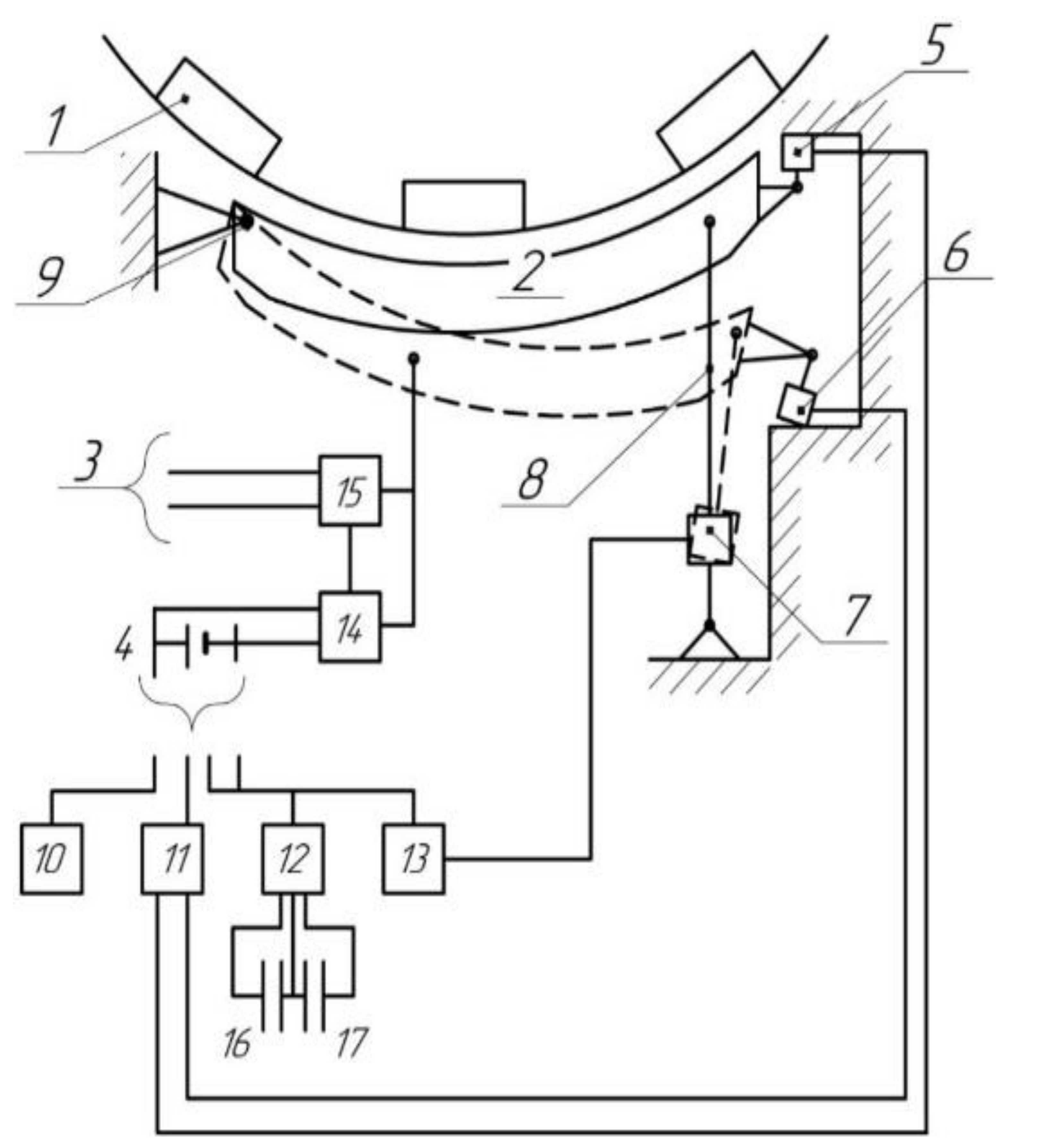
Figure 1), which interacts with the rotor element 1 of the wind turbine. Since the stator element 2 contains magnetic coils and permanent magnets, there is a significant radial force in the ‘rotor–stator’ complex, which prevents the functioning (rotation) of the rotor elements. Therefore, for example, in the period of no wind, it is necessary to reduce the radial force, which is possible only by withdrawal of the stator element. When the speed is increased, at sufficiently long wind impact, on the contrary, it is necessary to bring the stator element to the circle of the rotor element and to realize the release of energy to the network 3 or accumulator 4.
In general, the problem of regulating the flux of the permanent magnet is solved. Previously a demagnetizing winding was used, but this increased the consumption of copper for manufacturing. This article is a new way of flux control, which we are working out.
In “Selection of Electrical Generators for Wind Turbines” [
2], authors: Bubenchikova T.V., Molodikh V.O., Rudenok A.I., Danilov D.I., Shevchenko D.Y., various electric generators for wind power plants are considered. From the considered electric generators the synchronous generator with magneto-electric excitation is the closest to synchronous wind-electric generator of segmental type.
The advantages of an electric generator with magneto-electric excitation are:
Disadvantages:
The need to purchase expensive permanent magnets;
Constant magnetic flux, it is impossible to regulate it;
High cost;
Lack of domestic production base;
Demagnetization of magnets.
In wind turbine generator with movable stator segment there are no disadvantages described above. This device is cheaper in development, service life is doubled. However, the quality application of such a device requires a complex control system for maximum energy efficiency.
Advantages of a generator with a movable segment:
Precise control;
High reliability;
Low manufacturing cost.
Disadvantages:
To create a semblance of optimum control, as close as possible to the ideal current characteristic, we will use the circuit and description of the components shown in
Figure 1.
The electric actuator implementing the described method works as follows [
3]. The signal coming from the set point adjuster 10 comes to the regulator 11, which sends the signal to the input of the actuator 7 through the switch 12 and the converter (amplifier) 13. At the same time, this signal through the switch 12 is fed to the capacitor 16 and charges it. Drive 7 operates to bring the stator element to the rotor element until the limit switch 15 actuates. At that, on reaching the torque “t
s“, the switch, disconnecting the input signal, supplies to the amplifier 13 only the discharge signal from the capacitor 16, forming a quasi-optimal current diagram. If it is necessary to reduce the stop torque, i.e., when the stator element is withdrawn, the signal from the setter 10 is reversed, the process is reversed, except that to overcome the radial force of joint attraction of rotor and stator elements due to the presence of permanent magnets, the signal at time ‘t
s’ should be more intense.
2. Materials and Methods
For realization of optimum control for the purpose of minimum power consumption, it is necessary to stop on definition of transfer function of direct current electric drive (DC-motor). Non-zero initial conditions must be considered. At zero initial conditions it is physically impossible to make the motor rotate, the transfer function and its derivatives in time must be zero now the motion begins.
This is achieved because a capacitor (17) is included in parallel with capacitor (16), and, accordingly, the discharge effect will be more intense. Thus, we have two modes:
At the first stage, the stator element (2) is taken away from the rotor (1) to the extreme lower position (stop 6), which reduces the starting torque and allows the rotor to spin out at low wind speed.
After reaching a certain speed of the wind wheel, the electric drive of the stator segment (7) turns on and brings it closer to the rotor to the upper end position. This position is due to an approximately constant wind speed and maximum torque on the wind wheel shaft to give more energy to the electric grid.
Decrease of wind velocity leads to activation of electric drive of the stator segment and it is moving away from the rotor to stabilize torque on the wind wheel shaft, then the cycle is repeated as wind velocity changes.
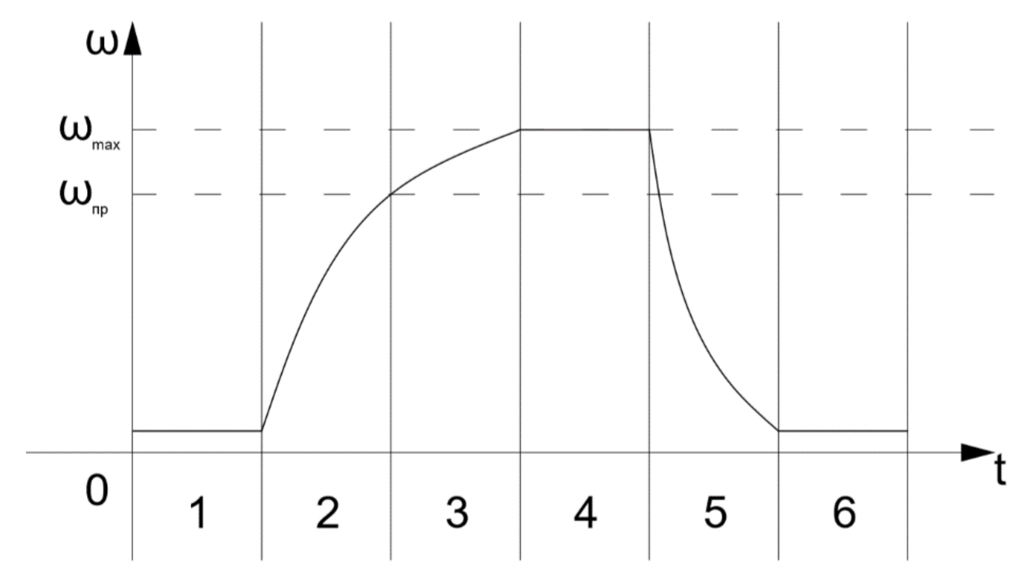
The paper [
4] shows a graph of the stator segment drive speed at different stages of operation: the full drive operation graph (2), during short-term wind action (3), during preventive shutdown (4), an enlarged start-up section to analyze preventive drive shutdown and drive up-drive of the segment by the self-running drive (5). We will use these graphs [
4] to analyze the drive operation and to work out the control signal of the future model.
Let’s consider the full schedule of the drive in
Figure 2.
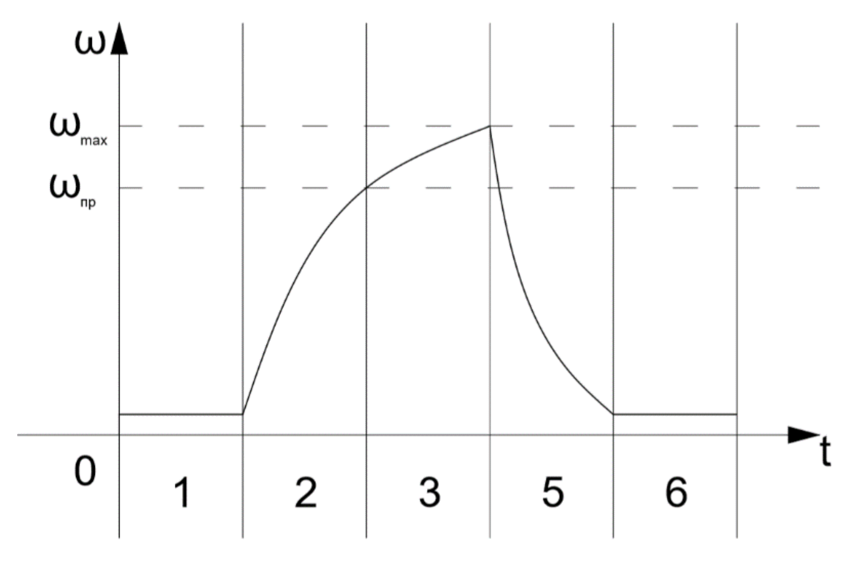
With a possible short-term exposure to wind flow, the section of algorithm 4 will be missing and the graph will look like this (
Figure 3):
Specific features of this actuator:
Small stroke (1–3 mm);
Significant dependence of the resistance moment on the sign of movement due to the presence of radial force;
Minimum power consumption, the control system components include an accumulator as a power source for the segment drive.
For implementation of the pilot plant, the drive type B-043.98105 was chose. This complete actuator includes:
This actuator was chosen because the whole power supply system of the stator segment is built at the voltage level of the car battery 12 V. B-043.98105 [
5] itself is the actuator of the ‘MINDA’ lock activator of the Daewoo Nexia car door and is well suited for realization of the required motion diagrams of the stator segment.
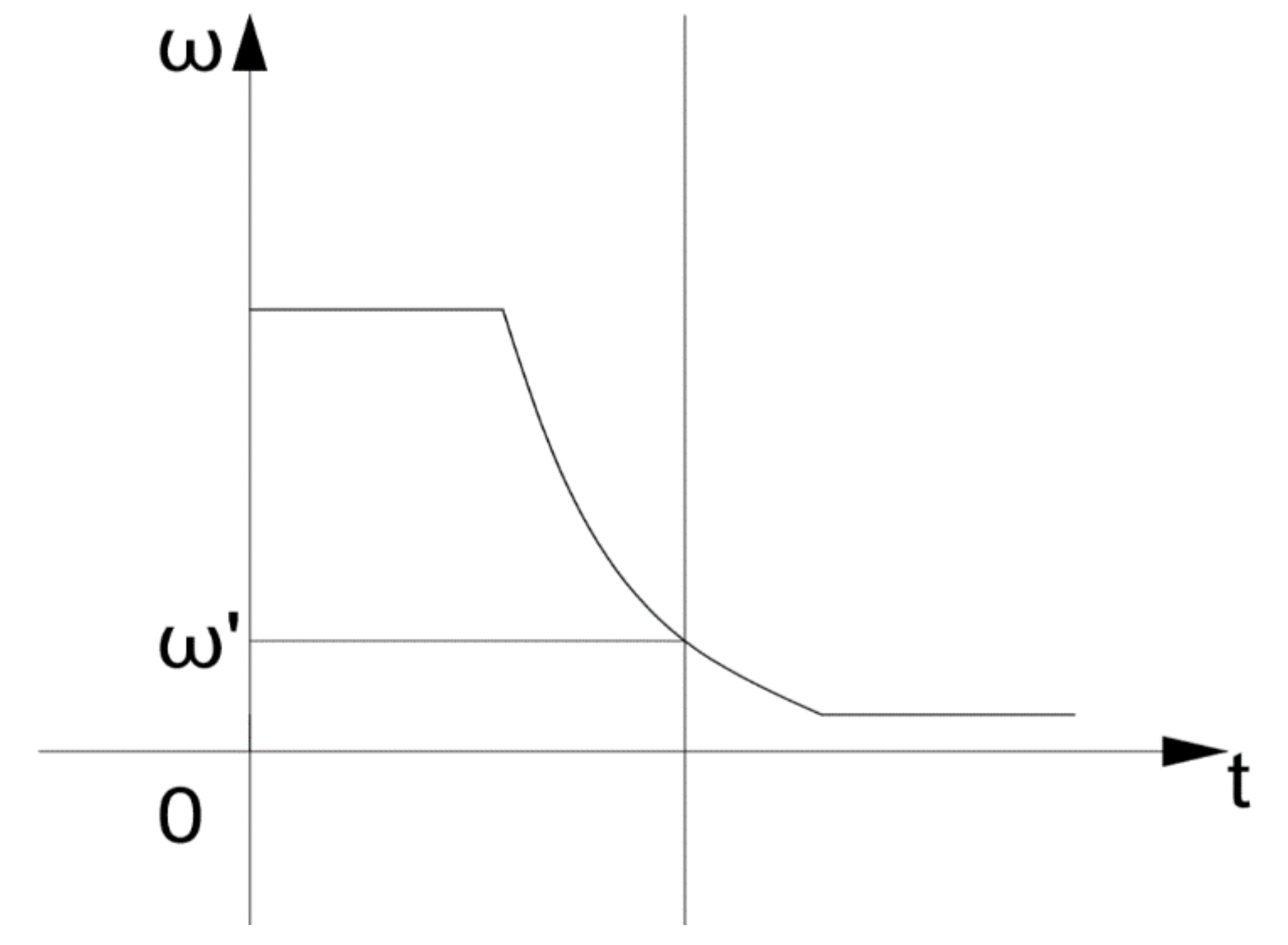
The moment of inertia of the armature is 0.0037 gm·cm
2 and the mechanical time constant is 0.05 s, due to which the coasting time can be taken into account when the stator is withdrawn and a trip earlier at wind wheel speed = ω’. The characteristic of velocity at preventive tripping is show in
Figure 4.
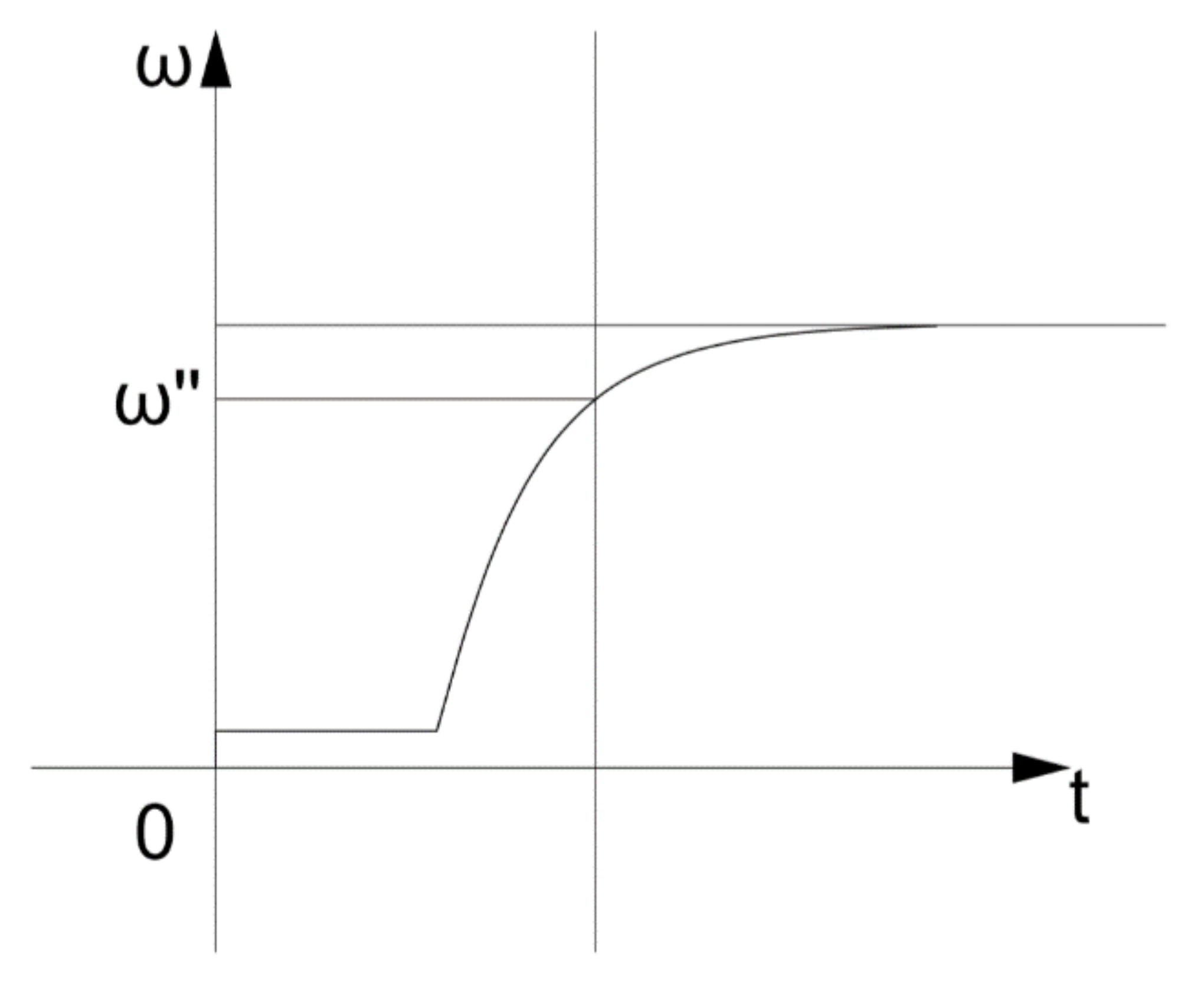
Provided there is no self-inhibition on
Section 1, it is possible to make a cutoff at speed: ω’’. The graph is shown in
Figure 5.
The scope of the drive is limited by the segment located between ω’ and ω”.
For further elaboration of the theoretical component of the simulation, we will use the calculation part of the article [
4], which describes the complete selection of the electric drive and control system based on the physical sense of the required transient process. Calculation concerns thermal, load and energy characteristics of the drive and is designed to minimize energy losses in wind turbine armature windings. Calculations result in determination of optimal stator segment displacement characteristic to optimize losses in wind turbine rotor.
The current speed diagram with five sections is known [
6]. Particular cases of such the speed diagram: three-part and in the limiting case-two-part the speed diagram of relay type.
The output of a drive is the stator angle of rotation, varying within a small range, up to 5° [
4].
In order to obtain an optimal drive diagram, it is necessary to minimize the load factor by heating:
—operating time;
—time of pause.
The loss of the energy in the armature winding;
According to [
4], we determine the loss of energy during one movement:
—is the static current;
—coefficient depending on the current form, in the optimal variant = 12.
Angle used by the motor shaft:
The angular constant of the actuator:
Divide the above expression by
+
, and we get the optimal program of the heating mechanism:
In this formula, x = 1, 2, 3 … R is the displacement number determined by the number of wind gusts and wind pauses per day.
Write setpoint controllers:
Here:
—movement of the working body, mm;
—total operating time, s;
—gear ratio of the gearbox;
K—guide vane number, mm/rev.
One duty cycle is not reversible, hence r = 1.
Substitute the expression for ω°:
This clearly shows the role of the moment of inertia included in the expression for .
In addition, the moment of inertia is included in the coefficient
which is part of the motor’s torque transfer function
Let the reduced moment of inertia be . We denote the coordinate of the stator segment rotation angle by x′. The coordinate x′ changes with time as the segment moves. The angular velocity of the segment will be the derivative of . Two external moments act on the segment: the friction torque- point of the stroke and the operating torque of the motor, and depending on the sign x point of the stroke, the radial impact from the rotor-Mg can be added to or subtracted from this torque. External moments act on the segment: the friction torque-in () and the motor operating torque–.
Thus, we have two equations
Assuming
, we write the law of motion as a system of differential equations
The quantities and are the phase coordinates, and is the control parameter.
The system then takes the form
Consider the problem when the endpoint is = (0, 0).
The Hamilton function according to the maximum principle has the form
and for the auxiliary variables
and
, we get
From here
where
,
—are constant integrations.
Furthermore, given the sign at
we have
that is
For a time interval in which
is identically equal to one, we have
Where
and
are constant integrations, hence
An arc of a parabola represents the segment of the phase trajectory, for this case, along which the representing points move from bottom to top, because
Similarly, for the case where
is identically equal to minus one, we obtain parabolic trajectories along which the points move from top to bottom (31, 32).
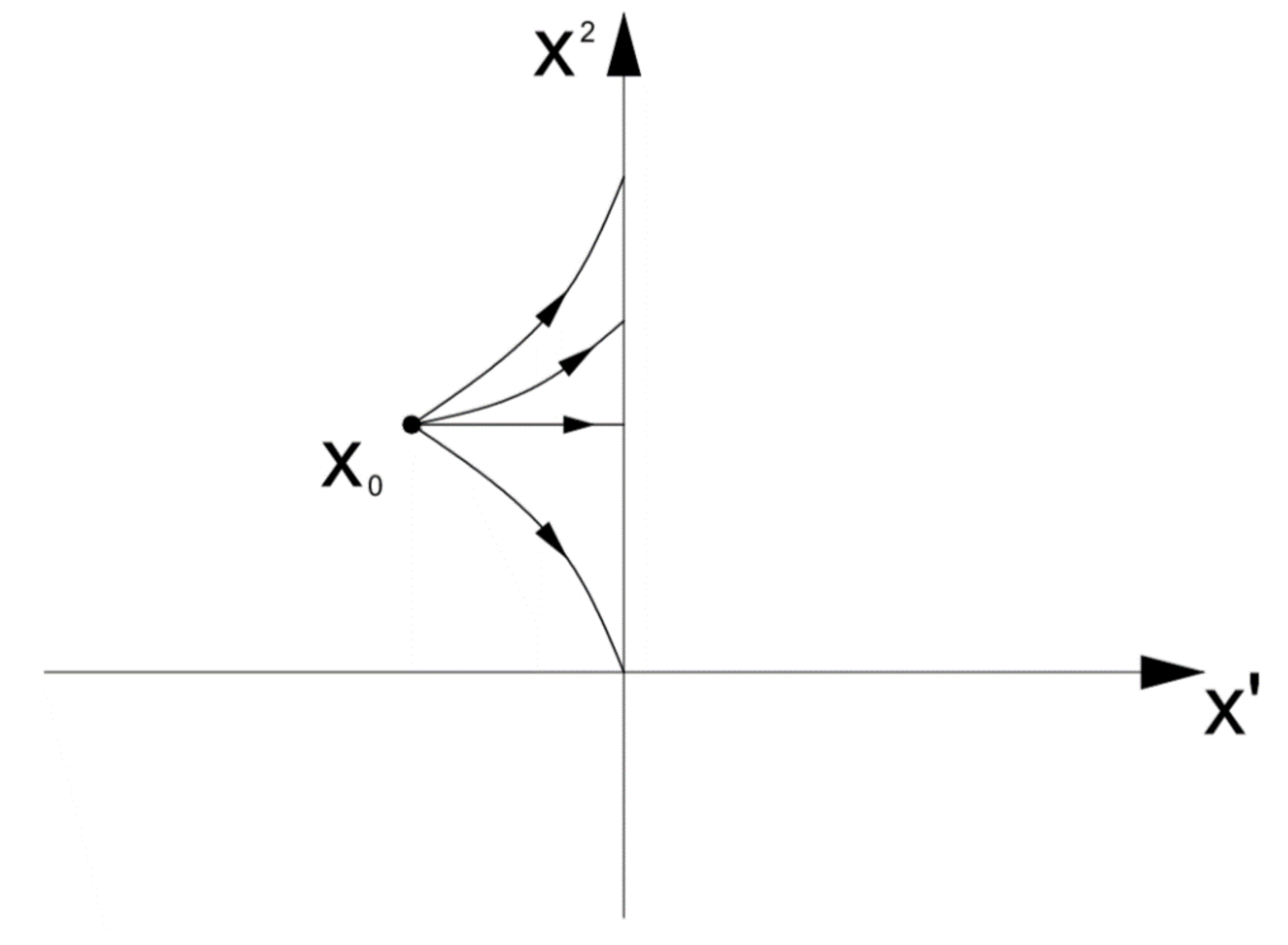
Figure 6 shows different control trajectories, the trajectory described above will be the lower one, the optimal control trajectory. The others lying above are direct start trajectories under different conditions.
Since the segment of the parabola for the optimal control passes through the origin of coordinates, its equation is (at u = −1)
In this case, at u = +1, the process will go from the fourth quadrant to the origin of coordinates
Thus, the optimal process actually occurs along the switching line, coinciding with the segments of parabolas [
6,
7].
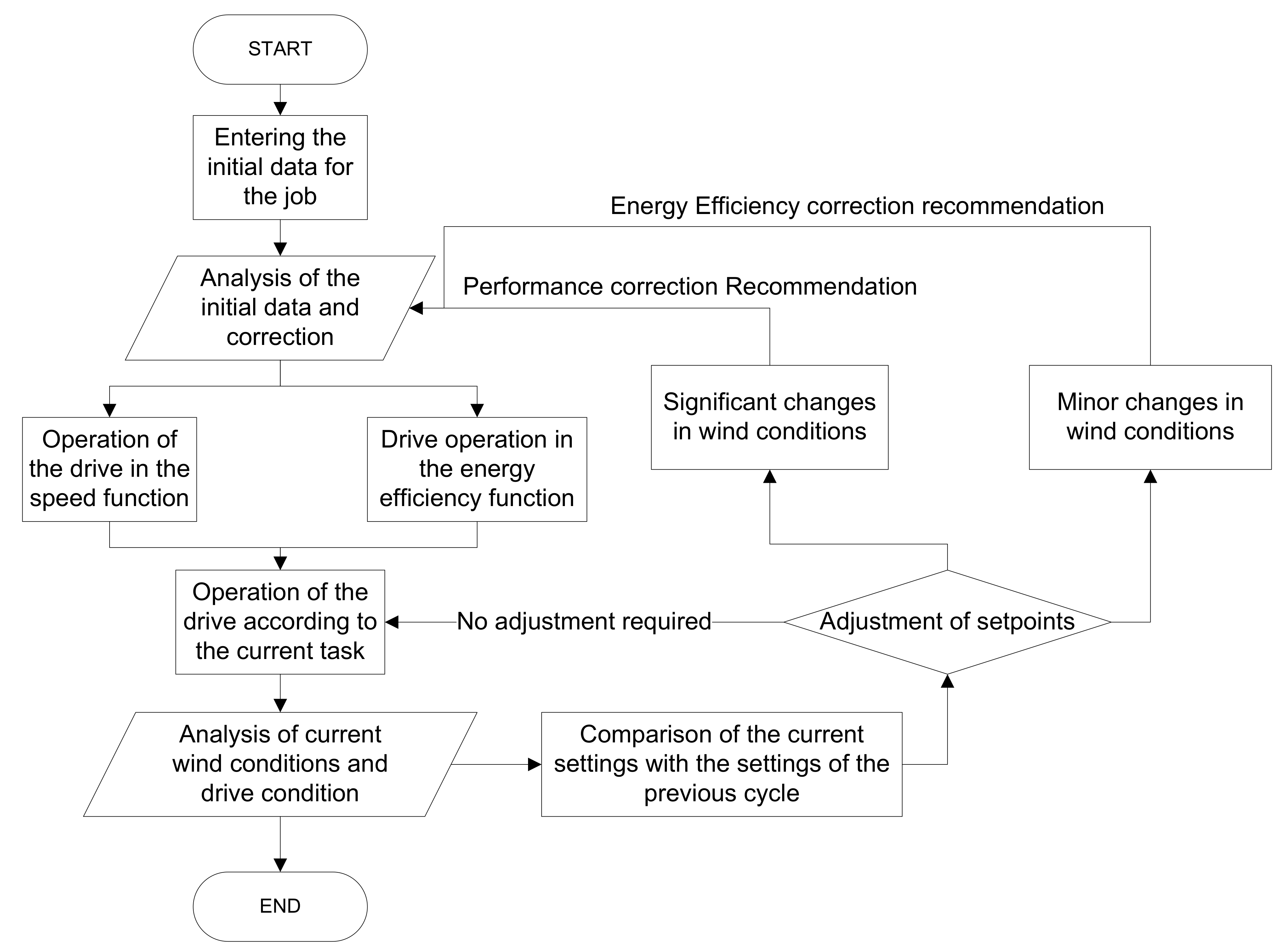
Taking into account the factors considered above, let us compose the drive algorithm, shown in
Figure 7.
The initial data of the drive operation involves entering the wind turbine parameters, wind speed based on the seasonality and prediction model, the initial position of the stator segment.
The block of data analysis and correction at the initial moment of time selects the drive function and gives the corresponding task. The blocks of drive functions in terms of speed and energy efficiency contain the corresponding characteristics of the task processing for the motion of the stator segment.
Then the reference run block sends the control action to the stator segment drive.
After the job is processed, the current wind conditions and the state of the wind turbine are analyzed. The following parameters are required for comparison:
It is also possible to add in parallel the wind prediction loop for some future period in order to proactively calculate the necessity of making adjustments in control parameter of the stator segment. This may require additional system parameters for comparison.
After comparing the data, the control system needs to decide if the segment control task needs to be adjusted:
If the wind wheel at the current wind speed can maintain the rotor speed near nominal, then no adjustment to the stator element is necessary, operate in the maximum energy efficiency function;
If the wind flow decreases and the wind turbine will not be able to maintain the required rotation speed, it is necessary to make a correction for the segment position.
At the same time, it is necessary to monitor the condition of the battery supply and make changes in the drive function based on this parameter. If the battery charge is satisfactory, the speed function can be applied, if not, the energy efficiency function.
The implementation of such an algorithm requires a large number of different analysis and prediction models. At this stage, we will limit ourselves to the implementation of an optimal regulator based on the principle of connecting a capacitor to the input of the inverter. This experiment is necessary to verify the feasibility of implementing a linear current diagram for this object. The segment control in the linear current diagram function is the basis of the drive operation in the energy efficiency function. Since the displacement of the stator element is a constant, two capacitors are connected to lead and lead off the segment.
3. Results
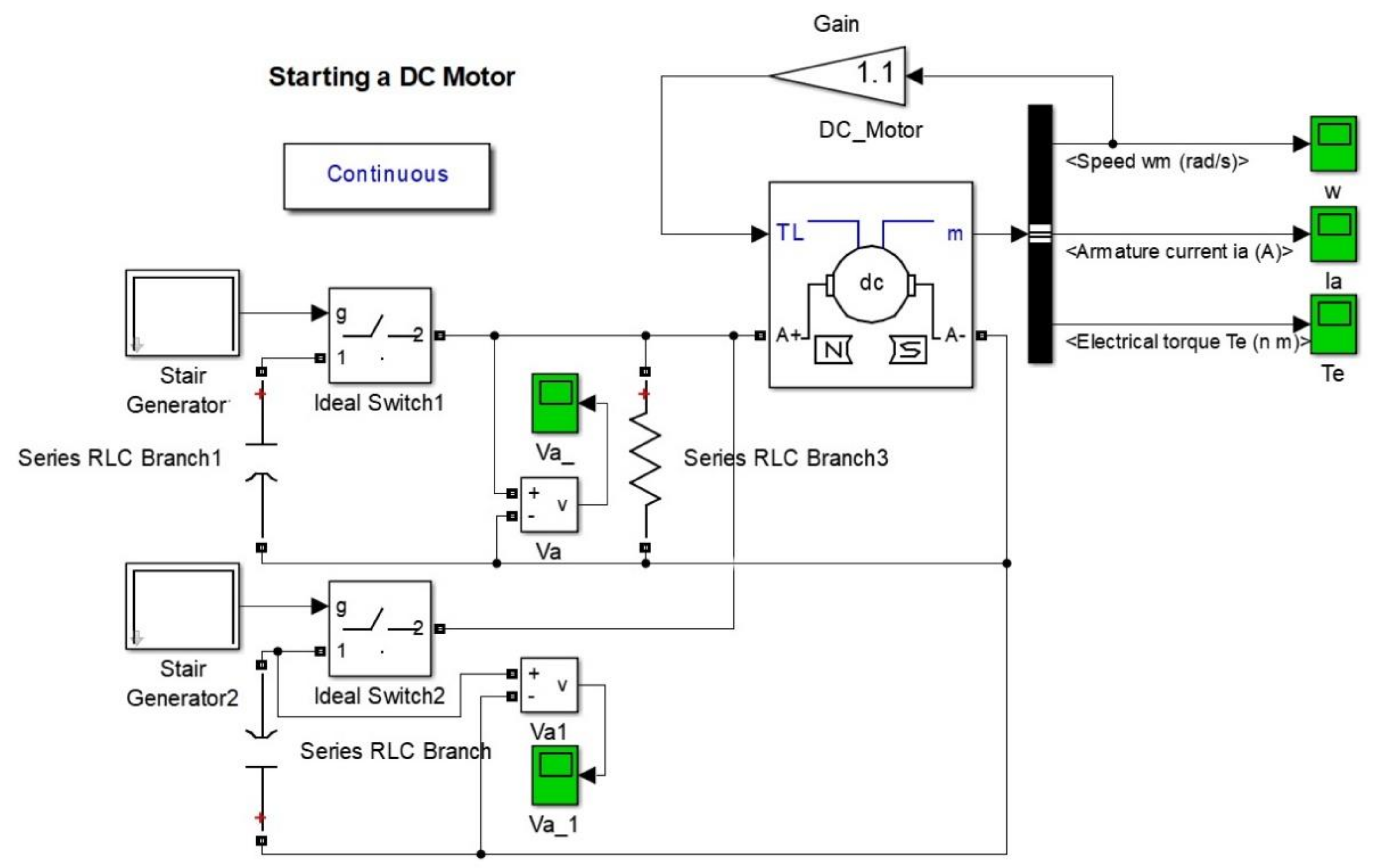
The implementation of this model should be checked in MATLAB environment. The structure of the model is shown in
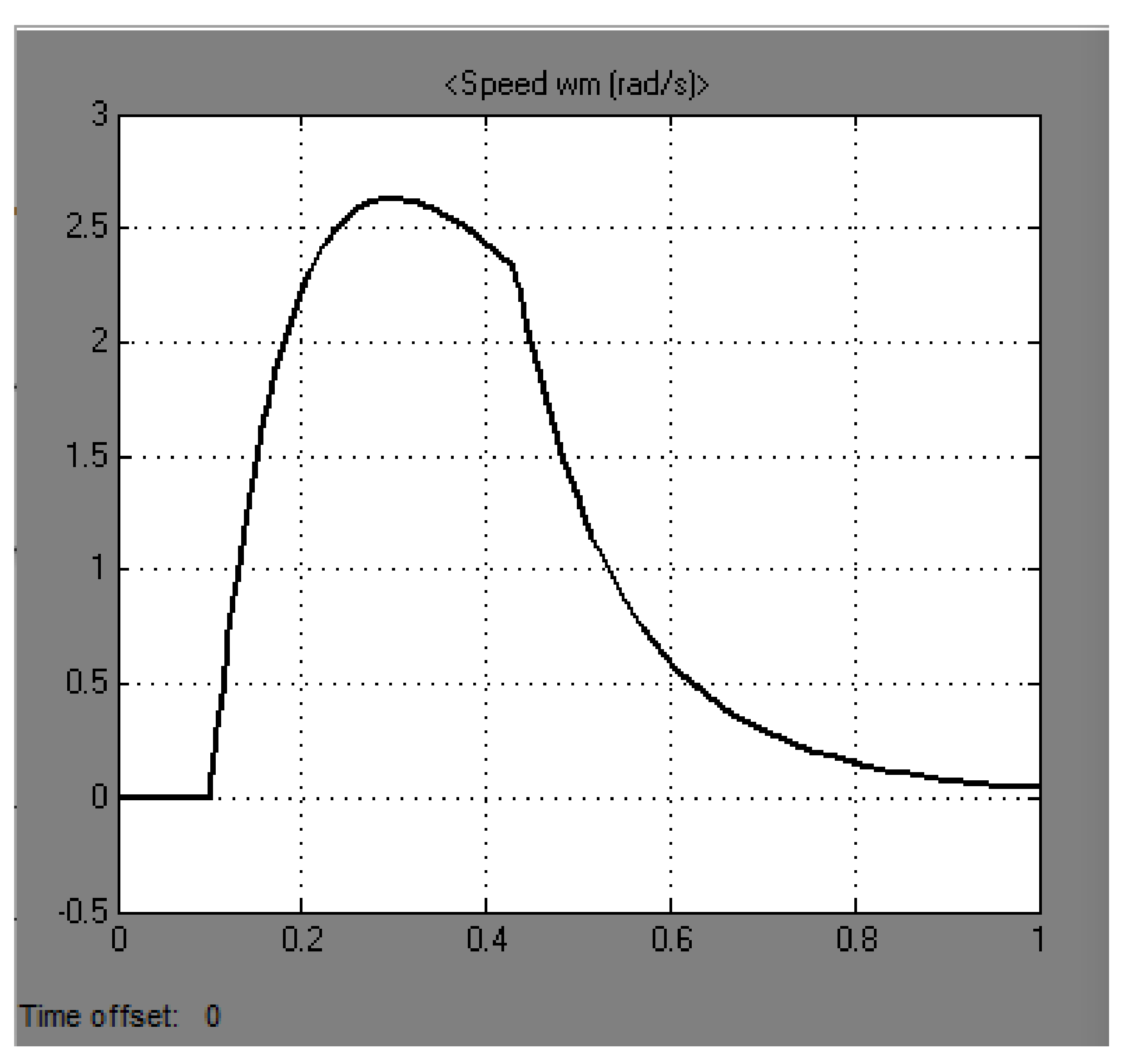
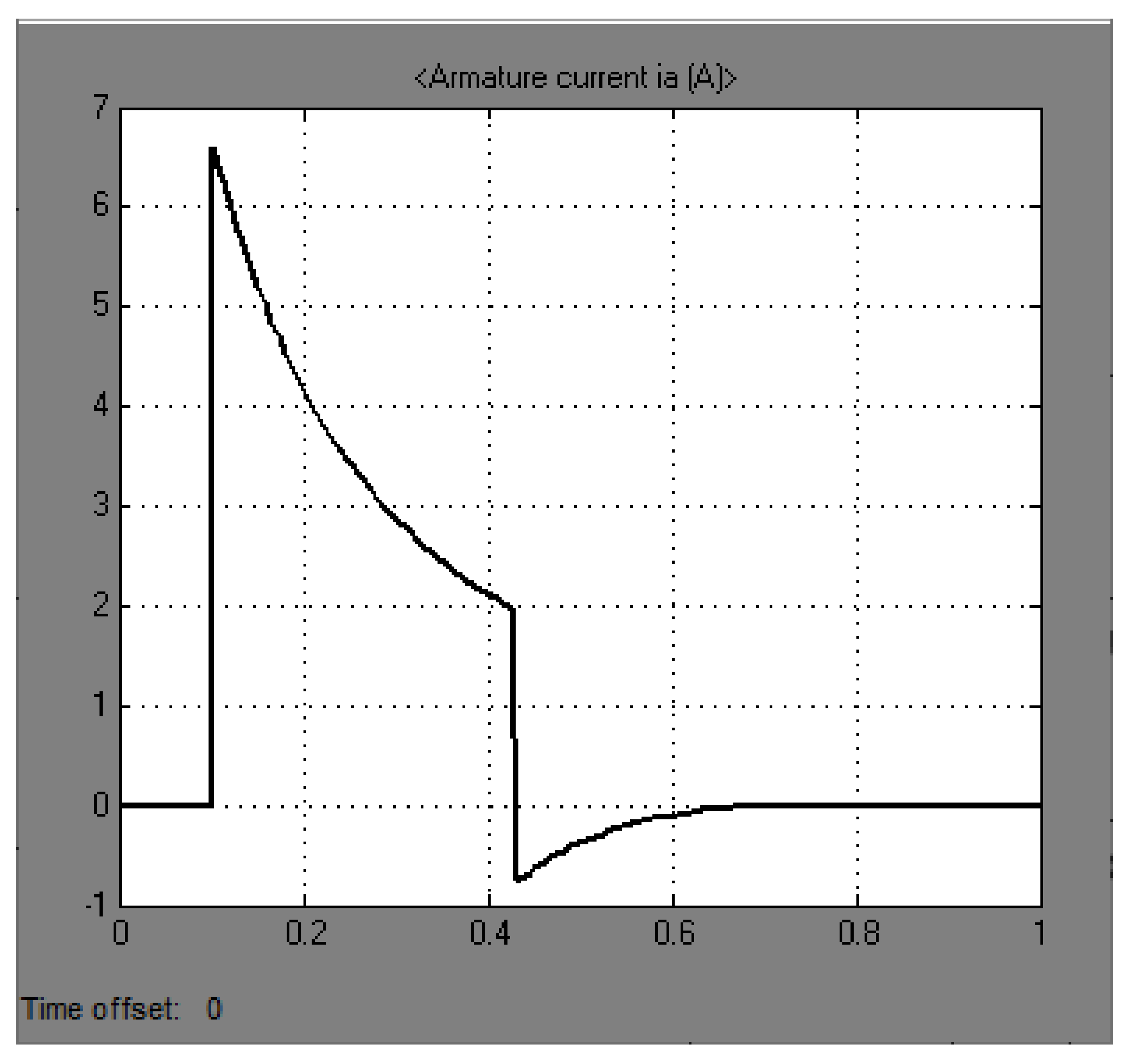
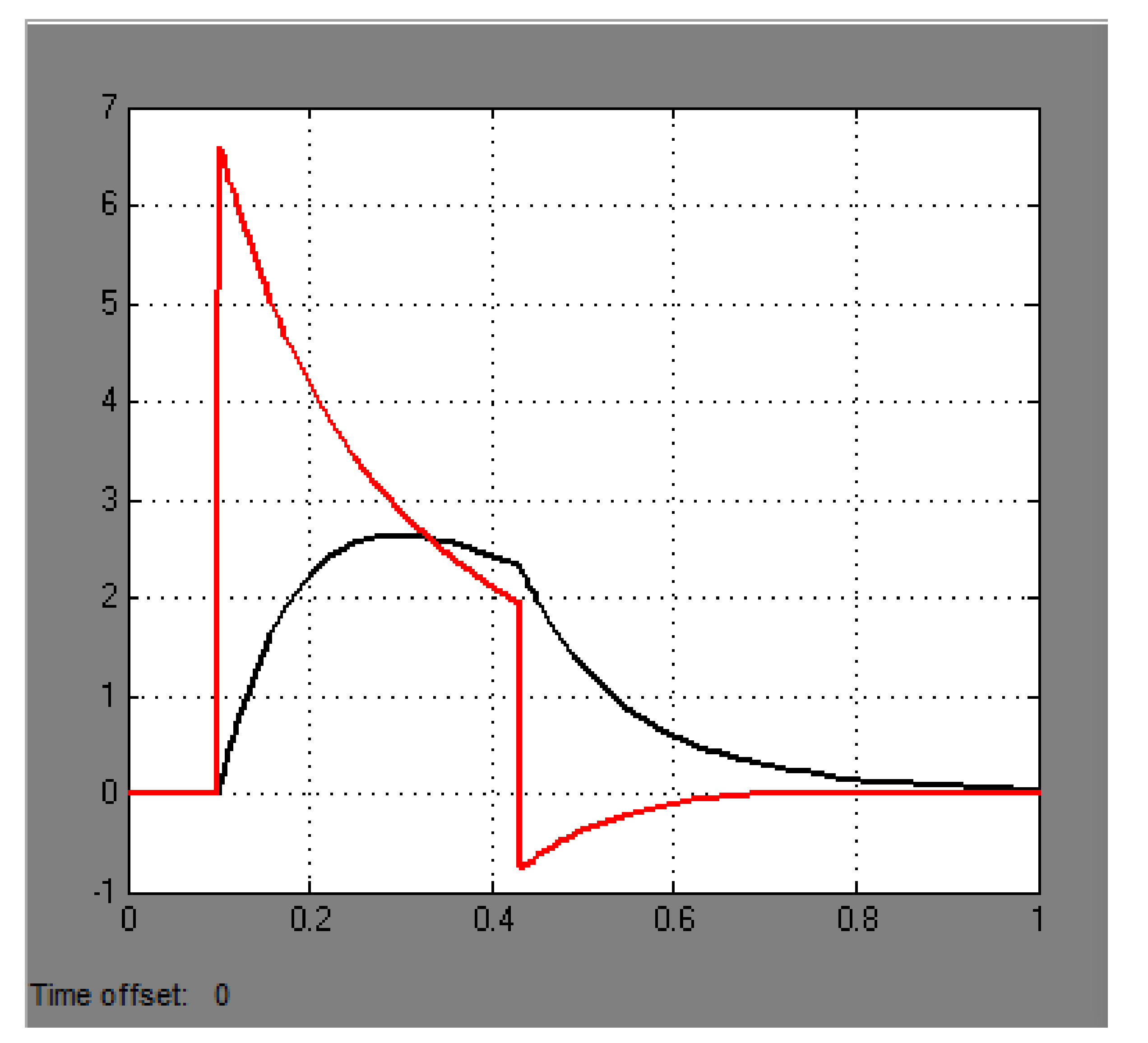
Figure 8. The resulting graphs are shown in
Figure 9,
Figure 10,
Figure 11.
The purpose of creating a model is to pre-test the hypotheses and conduct experiments without fatal consequences for the equipment. Based on the results of the simulation, an experimental model that confirms the implementation of the required control laws is to be assembled.
This model implements the segment drive algorithm described above. The composition of the model corresponds to a set of elements sufficient to implement optimal motor rotor current control. The model includes a direct current motor; capacitors supplying the armature when the drive is working to bring up and take down the WPG segment; control keys; blocks with a given control characteristic; voltage and current meters of the model; blocks of outputs of the main fixed parameters of the drive operation.
Table 1 shows the configuration of the motor unit.
This motor has a nominal supply voltage of 12 V, the moment of inertia of the armature is 0.0037 gm·cm2.
Graphs of the model operation when the actuator moves from stop to stop are shown in
Figure 9,
Figure 10,
Figure 11. In this experiment, we analyzed the transient process of actuator movement from stop to stop when the stator element of the windwheel is brought to the rotor.
From these graphs, we can judge about the adequacy of the model in relation to the calculations. For further analysis of the transient characteristics and it is necessary to build a prototype and evaluate the possibility of implementing the optimal control for the given actuator.
As an example of such a drive can be the stator drive of segmental inductor wind turbine generator [
1], the movement of which manages to regulate the magnetic field of permanent magnets. This principle will be considered on the example of the drive of the stator element of the segment wind turbine generator, which interacts with the rotor elements 1 of the wind turbine. Since the stator element 2 contains magnetic coils and permanent magnets, there is a significant radial force in the ‘rotor–stator’ complex, which prevents the functioning (rotation) of the rotor elements. Therefore, for example, in the period of no wind, it is necessary to reduce the radial force, which is possible only by retracting the stator element.
A further consideration should be taken into account for both drive modes in the end positions of the outer stator. It concerns the consideration of the kinetic energy of the rotating parts of the actuator, especially the rotor. This determines the distance between the main sensor and the intermediate stop sensor.
In order to realize an optimal control in the function of minimum power consumption, it is necessary to stop at determining the transfer function of the DC-motor, it is necessary to [
8]:
Consider non-zero initial conditions (at zero initial conditions it is physically impossible to realize motor start);
The transfer function and its derivatives in time must be equal to zero at the moment of start of motion.
An ideal current diagram is shown in
Figure 12.
On the basis of relative units, you can create the equation [
2,
3]
where
Axx,
Bxx,
Cxx,
N—constants.
From the moment of starting, these equations are joint, and taking into account the general equation of engine speed (moving to the Laplace image), we have
taking into account the provision of a jump-like increase in the initial starting current and initial acceleration when the voltage is applied
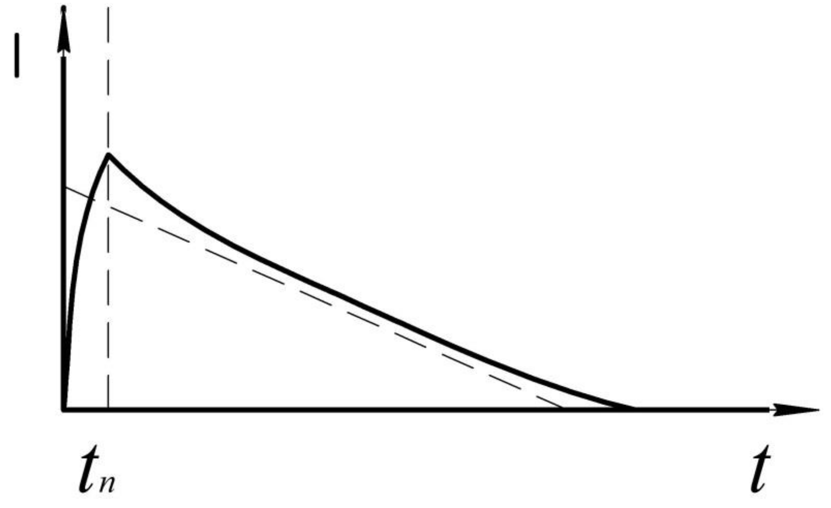
In this presentation, we are interested in the diagram of current changes. From the known literature, we can distinguish several approaches to the formation of a current diagram, and the associated diagram of speed changes. According to [
8,
9], this diagram is linear, and the velocity change diagram is parabolic
The law of current change is also known [
9]. The velocity change diagram has a decrease in the maximum in comparison with the parabolic one, accompanied by its flattening
In this regard, it should be noted that these and similar diagrams are theoretical in nature, but in reality, only a certain approximation to the optimal dependence can actually be synthesized.
Implementation can be carried out in different ways. Therefore, in [
10,
11], it is indicated that at the initial moment the maximum voltage should be applied to the armature, and as soon as the current reaches the optimal value, the voltage is reduced, and then at the end of the cycle the maximum voltage of the reverse sign is applied. That is, in this case, we have two commutations, in addition, in the end, the regularity of the current change after the first commutation is not clear.
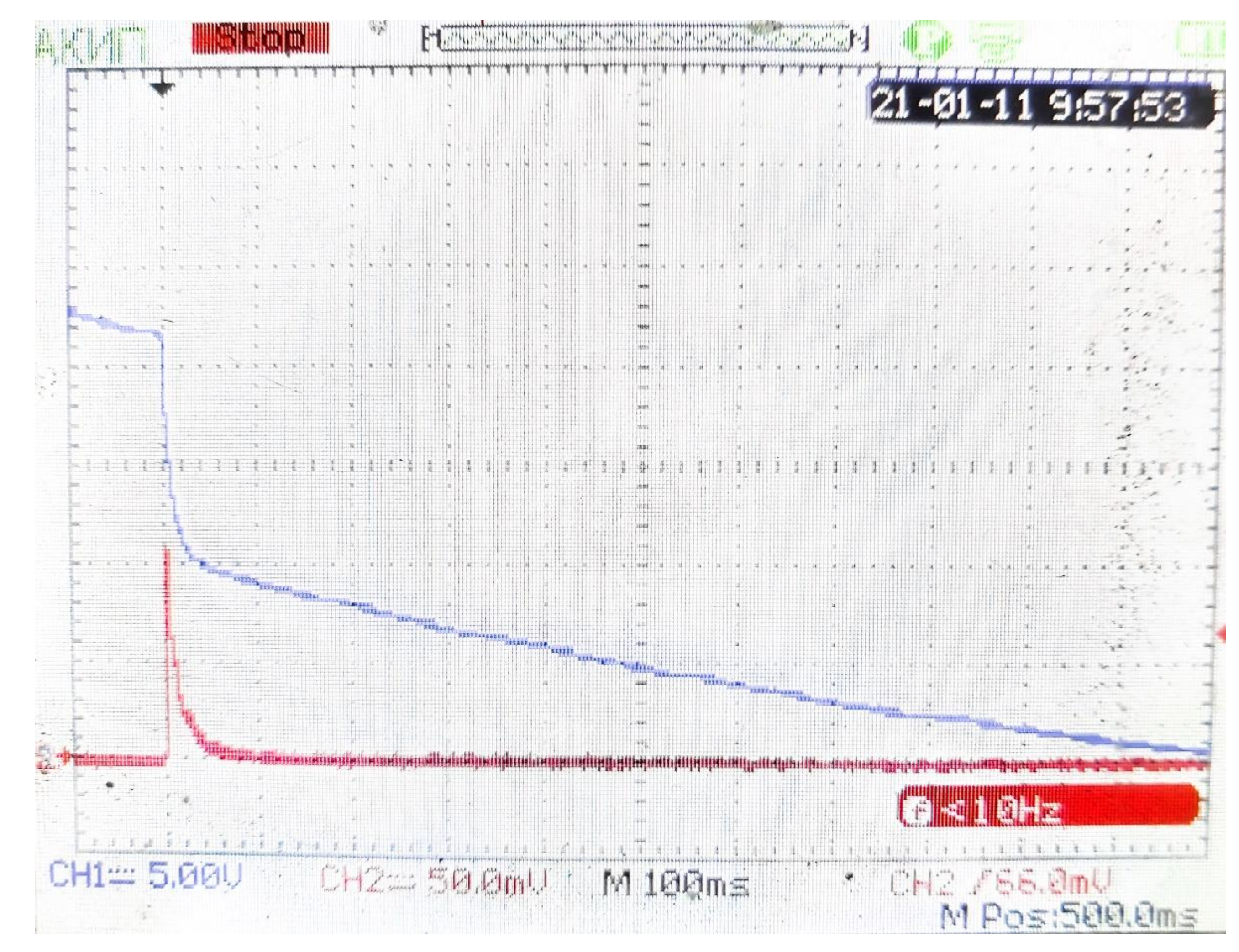
The implementation of the current diagram on a real object is shown in
Figure 13 in an enlarged form. The graph in blue corresponds to the voltage on the capacitor, red indicates the current consumed by the motor.
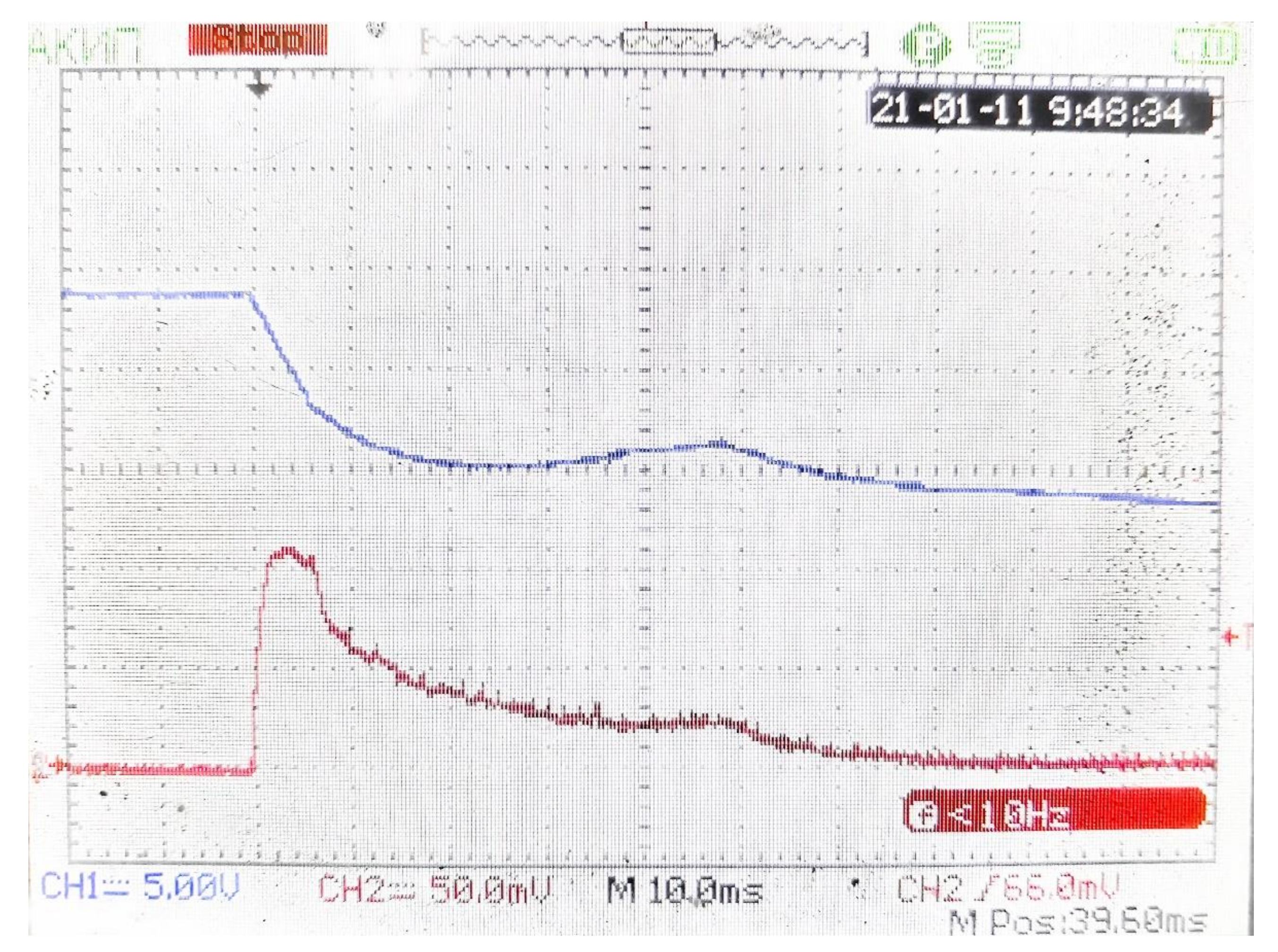
The implementation of the current diagram on a real object is shown in
Figure 14 in an approximate form.
The measurements were carried out using an AKIP-4125/1A digital oscilloscope [
12]. This device has two adjustable measurement channels. The first channel (blue graph) recorded voltage values at the feeding capacitor, the level of charging voltage is higher than the level of the actuator drive supply voltage and is 20 V. At the moment of the actuator start, the voltage sag and the moment of the capacitor self-discharge after the motor braking and disconnecting it from the capacitor supply circuit can be seen.
The second channel recorded the motor current (red graph). For measurements, we used ATK-2001 current clamps with an adapter for AKIP-4125/1A oscilloscope. The signal from the current clamps comes in the form of normalized voltage and is 25 mV per 1A, therefore, the motor current was 4.2 A. For clarity, both graphs are placed on the same plane with different spacing:
Figure 13—100 ms. in one cell,
Figure 14—10 ms. in one cell.
The MATLAB model uses a return capacitor, which stores the braking energy of the drive. Only one capacitor was mounted on the real installation to start the drive. The transient time of the real plant without the braking capacitor was 50–60 ms.
When simulating in MATLAB with the brake capacitor, the transient time to work out the task is 20 ms. Taking into account the absence of the second capacitor for accumulation of braking energy of the motor, the results of mathematical modeling and graphs of the implemented installation can be considered identical.
At the initial moment of time, the capacitor is charged, the motor is disconnected from the capacitor. There is a small voltage drop on the capacitor due to self-discharge. Then, the motor is connected and a current is generated in the circuit that corresponds to the required diagram. After the set point has been reached, a signal is given to disconnect the motor from the power supply circuit, the current in the circuit disappears and the final discharge of the capacitor takes place.
4. Discussion
At the initial moment of time the capacitor is charged, the motor is disconnected from the capacitor, there is a small voltage drop on the capacitor due to self-discharge. Then the motor is connected and the current in the circuit coincides with the required diagram. After the task is completed, a signal is sent to disconnect the motor from the power supply circuit, the current in the circuit disappears, and then the final discharge of the capacitor takes place.
According to the results of simulation, linear current and speed diagrams have been realized with application of optimum control, this type of control can be applied on drives of other classes. The realization of this installation confirms the applied laws and control methods in relation to the current diagram of the electric drive of the wind turbine segment; the simplification of realization affects the deviation from the ideal current diagram by 11%, which is acceptable for this installation. Since the control system on the simplest electrical elements was used to implement the current diagram, 11% deviation is acceptable. The essence of further work is to minimize this percentage of deviation; however, as practice shows, the minimization of 11% deviation from the ideal current diagram will require appreciation of both the element base and the control system. In further research, the start and pause times are set as a function of the mean annual wind speed pattern and can be predicted by a neural network.
At present, the task of collecting wind speed data to train a neural network that predicts the speed and direction of wind flow and to perform a task for optimal control of the stator segment has already been solved.
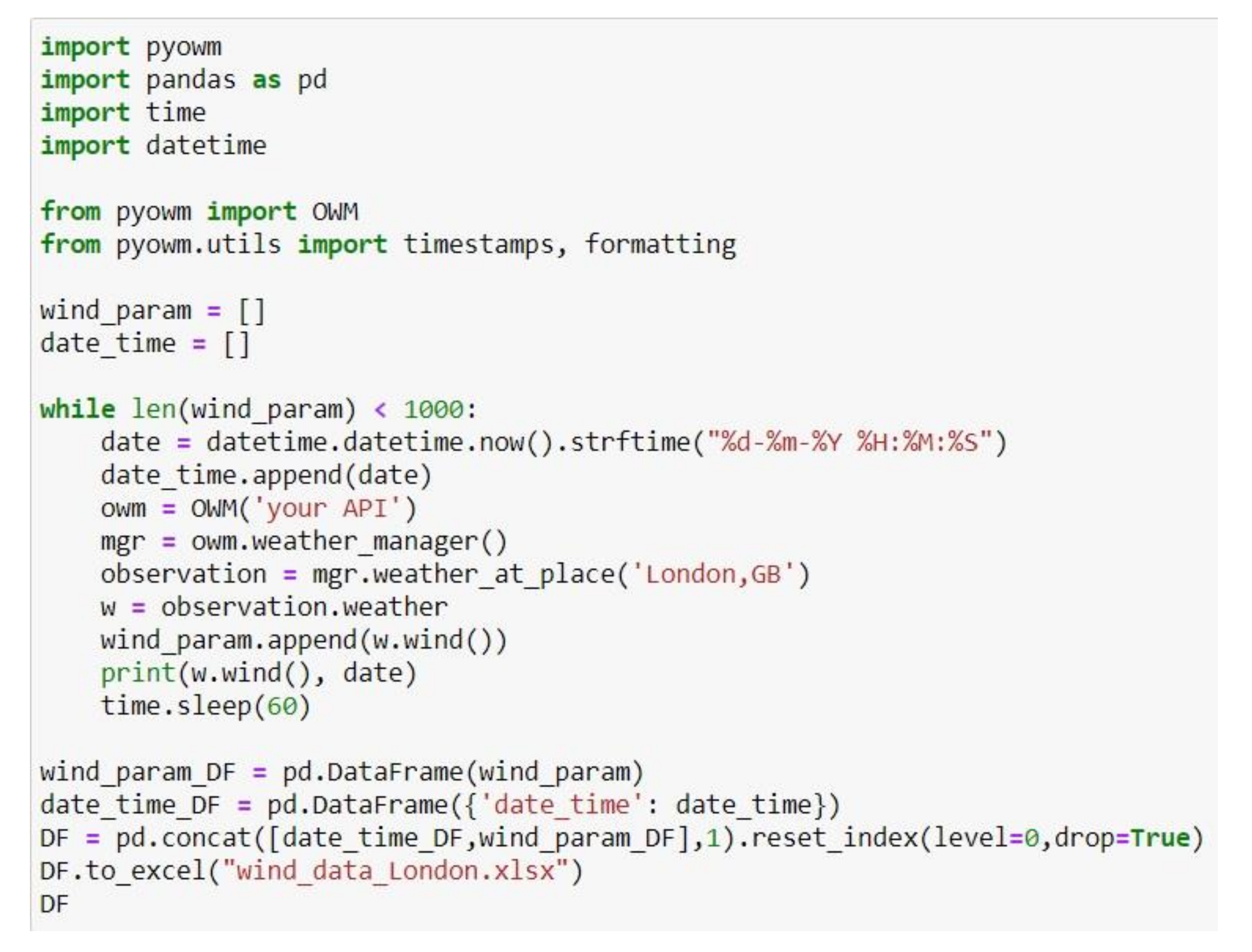
The data collection and processing task has been implemented in a python program code. Thanks to the openness of the research community, some companies provide various data on a royalty-free basis, which may be necessary for scientific research or the creation of software products. For example, the Open Weather Map [
13] information portal, which collects, stores and processes information from all meteorological points around the world, provides free access to some data via an API key. This company presented the pyowm package [
14] for the python programming language, which allows you to quickly and easily make requests to the server and get the required information.
We created a program that collects the necessary data and creates an excel file from them. Furthermore, it is convenient to work with this file and form data sets for training and checking the neural network, and to build graphs.
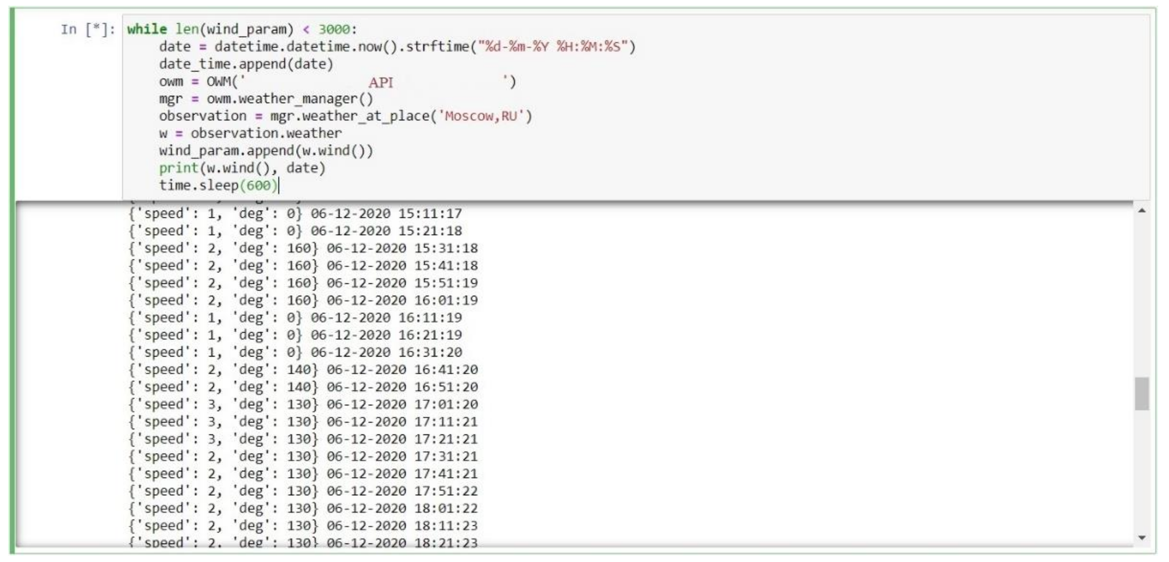
The result of the program operation is a data table consisting of the given number of rows and columns with wind parameters and measurement time. The intermediate output of the program is shown in
Figure 16.
This figure shows the sequence of data lines outputted by the program. In curly brackets, the dictionary with wind speed and degree of direction is marked, then the date and time of parameters recording is output.
Table 2 shows the result of the part of the program that generates the excel document.
The obtained data allows analyzing the wind speed and forming the training and test samples for the neural network model of wind speed prediction and stator segment control.
5. Conclusions
According to the results of simulation, linear current and speed diagrams were implemented using optimal control, this type of control can be applied to drives of other classes. The implementation of this installation confirms the laws and control methods used in relation to the current diagram of the electric drive of the wind turbine segment, the simplification of implementation affects the deviation from the ideal current diagram by 11%.
In terms of reference, it was established that the deviation from the ideal current diagram is not more than 15% at this stage of development. At this stage, it was required to solve the scientific problem of stator segment motion optimization and achieve the deviation minimization.
As the control system on the simplest electric elements was used for realization of the current diagram, 11% deviation is acceptable. The essence of further work is to minimize this percentage of deviation; however, as practice shows, the minimization of 11% deviation from the ideal current diagram will require appreciation of both the element base and the control system. In further research, the start and pause times are set as a function of the annual average wind speed pattern and can be predicted by a neural network.
At this point, the optimal control problem in the special case characteristic of the unique reversible position control object under consideration is solved. This object is characterized by different equations for operation in modes of proximity and distance of stator segment from wind wheel rotor Equations (35) and (36). An algorithm and the corresponding model were compiled.
Analysis of simulation results showed that the proposed control provides satisfactory performance for given parameters. Besides, realization of optimum control on the real sample of the drive was considered (
Figure 13 and
Figure 14), where quantitative dynamic dependences which satisfy the set parameters are reflected. It is established, that the received model adequately reflects processes in the object.
Physical modeling was performed on a 20° segment; application of this module is also possible for slow-speed wind generators with installation of up to 18 such modules on the circumference.


