Numerical and Experimental Study of a Device for Electrical Power Lines Probing for a Tunnel-Boring Complex Control System ^†

Abstract

The article considers the problems of the magnetic field distribution, generated by a power electric cable at the micro-tunnel-boring shield arrangement site by numerical modeling with a further full-scale device model experiment. The impact of foreign magnetic field sources on readings of three-component sensors was established in the process of the study. The considerable existence of parasitic noises, conditioned by external magnetic fields and high sensitivity of the probes, which will require the use of additional filters, was established. When using three-component ferroprobes, the most informative is the probe component coinciding with the tunnel shield longitudinal axis Z. The study showed that with current values greater than 200 A and changes in cable location during the experiment, it is possible to record signals from other sensor components and subsequently determine the location and orientation of the current-carrying cable. The experimental results obtained confirm the feasibility of a multi-sensor probing device for the micro-tunneling machine shield movement control system.

1. Introduction

During the construction of municipal gravity and pressure sewerage systems, heating mains, gas pipelines and other underground utilities, micro-tunnel-boring machines (shields) are used [1]. At the same time, during subsurface tunneling operations, it is important to detect power electric cables in the ground to protect workers, tunneling equipment and power system equipment from electric shock. It should be noted that in big cities most power cable routes are located in the ground, and the total number of performed excavation works in municipal areas in developed countries may exceed several million [2]. This work was carried out as part of a project to develop a micro-tunnel-boring shield for tunneling 1.4 m in diameter for supply utilities of various purposes. In this case, the customer’s requirement for the probing system was to be able to be installed on the micro-tunnel-boring shield and to be able to detect power cable lines along the boring path.

2. Applicability

Because the operation of the complex is assumed in the territory of industrial zones and urban development, the probing of power cable lines from the daylight surface in some cases is not possible. Back in the early 1980s, subsurface probing systems (for example, BoRaTec [3,4]) were presented, but they did not allow probing along the trajectory of the boring without restrictions. In 1997–1998, the BEAM [5], TRT [6], SSP [6] and TR-GEO-01 [7] systems were presented, which allow detecting communications on the tunneling trajectory. These systems use georadiolocation or seismic-acoustic methods to detect underground supply utility constructions.

As a rule, such systems have a low resolution (0.5–1.5 m), which does not allow detecting power cable lines in a number of cases. For example, in the case of a cable line laid outside the cable tray or in a small cross-section (0.3 × 0.3 m) concrete cable tray. In addition, the negative impact on the quality of probing can significantly worsen when working on waterlogged soil, the impossibility of ensuring a close contact of the probe emitter with the soil, structurally inhomogeneous soil, etc. For this reason, as well as to meet customer requirements, a magnetometric probing method [8] for power cable line detecting was chosen.

Modern works, addressing the detection of underground power cable lines, focus not only on the spatial arrangement of the power cable but also on possible parameters of the power cable line [9,10,11,12]. However, it is not necessary to determine the power cable parameters during tunneling operations; it is sufficient to record its arrangement in the ground and its orientation relative to the tunneling shield to ensure safe tunneling operations [13,14]. At the same time, it may be difficult to detect the arrangement of power cable lines due to present major construction objects above the worksite or by a considerable depth of tunneling operations, preventing cable line detection from the daylight surface [15,16]. In such cases, due to the small size of the tunnels, magnetometric sensors can be arranged right only on the micro-tunnel-boring shield and can complement or be integrated into the existing advanced multi-sensor daylight surface probing system [17,18,19] to detect power cable lines.

Thus, until now, such probing systems have not been used as a part of the micro-tunnel-boring shields. The aim of this project considered the creation of a new probing system designed to be installed on tunnel-boring shields (diameter 0.9–1.5 m). Such a system is compact in size, but due to the chosen probing method, it is designed only for use in urban areas and industrial zones. This is due to its ability to detect power cable lines, steel pipelines, steel and reinforced concrete structures and its inability to detect natural obstacles (cavities, rocks that are too strong, etc.). Unlike earlier studies, in the project of this paper, we considered a wider range of currents in the cable and put full-scale experiments on full-size dummy micro-tunnel-boring shield housing.

3. Problem Formulation

The present work studied magnetic field distribution, generated by a power electric cable at the front of the micro-tunnel-boring shield, and determined the possibility of its detection using magneto-sensitive shield sensors. The problem was solved by numerical simulation with a further experiment.

The problem under consideration is a common application of the Biot–Savart–Laplace law. In the general case, the source of the electromagnetic field is an extended conductor with the current. The value of the magnetic induction at any point in space can be calculated in accordance with the equation of the law:

$$\mathrm{d}\overrightarrow{B}=\frac{{\mathsf{\mu }}_{0}i\mathrm{d}\overrightarrow{s}\times \overrightarrow{r}}{4\mathsf{\pi }{r}^3}$$

(1)

where µ₀–vacuum permeability, i–current value in the conductor, ds–conductor element, and r–full displacement vector from the wire element (ds) to the point at which the field is being computed.

The analytical method for calculating the value of magnetic induction was used to verify the mathematical and numerical FEM models of the three-dimensional computational domain in the work [9].

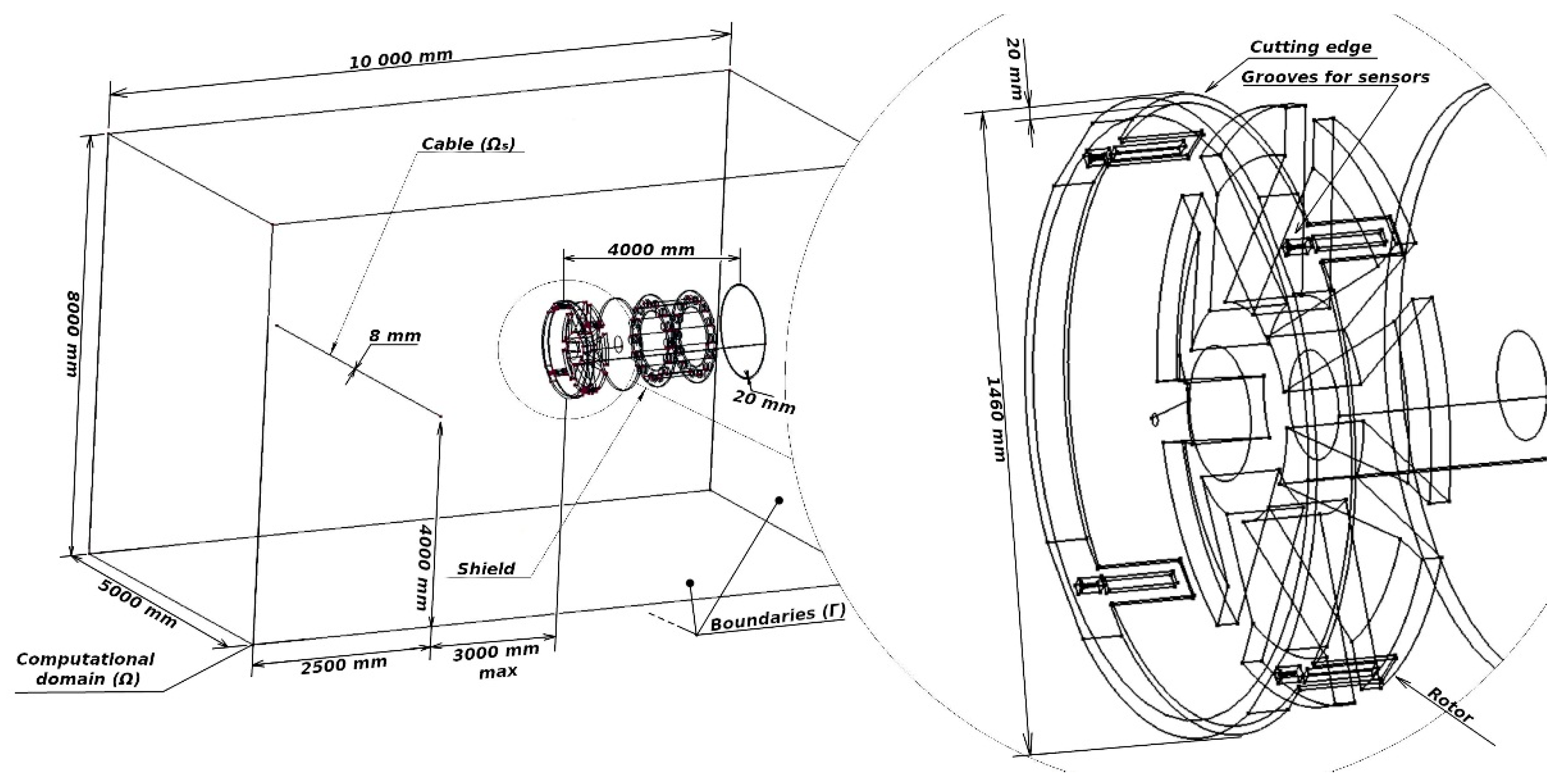
To simulate a magnetic field topology, the three-dimensional computational domain was used. It was bounded by the rectangular parallelepiped, 17 × 10.5 × 8.5 m in size (Figure 1). The computational domain contains a power cable with a diameter of 8 mm (straight cylinder) and massive ferromagnetic parts (supporting structural elements, rotor and its drive) of the micro-tunnel-boring shield. The shield body is made in the form of a pipe with an outer diameter of 1.42 m, a length of 4 m and a wall thickness of 20 mm.

The a-formulation of the electromagnetic field is obtained from the weak form of the Ampere Equation:

(ν curl a, curl a’)_Ω − (j_s, a)_Ωs = 0

(2)

where a—magnetic vector potential, Ω—bounded computational domain, ν—magnetic reluctivity, and j_s—current density in the source domain Ωs.

At the boundary Γ of the computational domain Ω, the Dirichlet boundary conditions are applied (the values of the vector magnetic potential are reduced to zero). To reduce the computational complexity of the process of solving a system of linear equations, the tree-cotree gauge [20] was applied, which ensures the regularization of the matrix of unknowns.

To solve the numerical simulation problem, the software complex GMSH+GetDP was used [21,22]. The finite element mesh was created by using the GMSH mesh generator utilizing the algorithm Frontal [23] for 2D objects and HXT for 3D objects [24]. The finite element mesh contained nodes and 8.5–10.2 mln. tetrahedrons with linear sizes of edges from 1.75 to 400 mm.

For ferromagnetic elements of the micro-tunnel-boring shield structure, the nonlinear magnetic characteristics were set as for steel 1020.

The system of linear equations consisted of 5.02 − 5.3 × 106 equations. The density of the matrix of unknowns is about 0.00014–0.00015%. The solution of the numerical problem was performed in the GetDP environment using the MUMPS solver [25] (as part of the PETSc toolkit [26]). Nonlinear problem was solved by the Newton–Raphson iteration with the intermediate solving the simultaneous linear algebraic equations using the Cholesky method (OpenBLAS [27] routines for SLAE solving was used) with ordering by the METIS algorithm [28]. Time for calculating the magnetic field was 0.5–1.5 h for each shield position (PC with FX-8320E processor, 32GB RAM and 240GB SSD storage for out-of-core factorization). In all cases, the solving of a nonlinear numerical problem required 2–4 iterations to achieve an error of 0.1%.

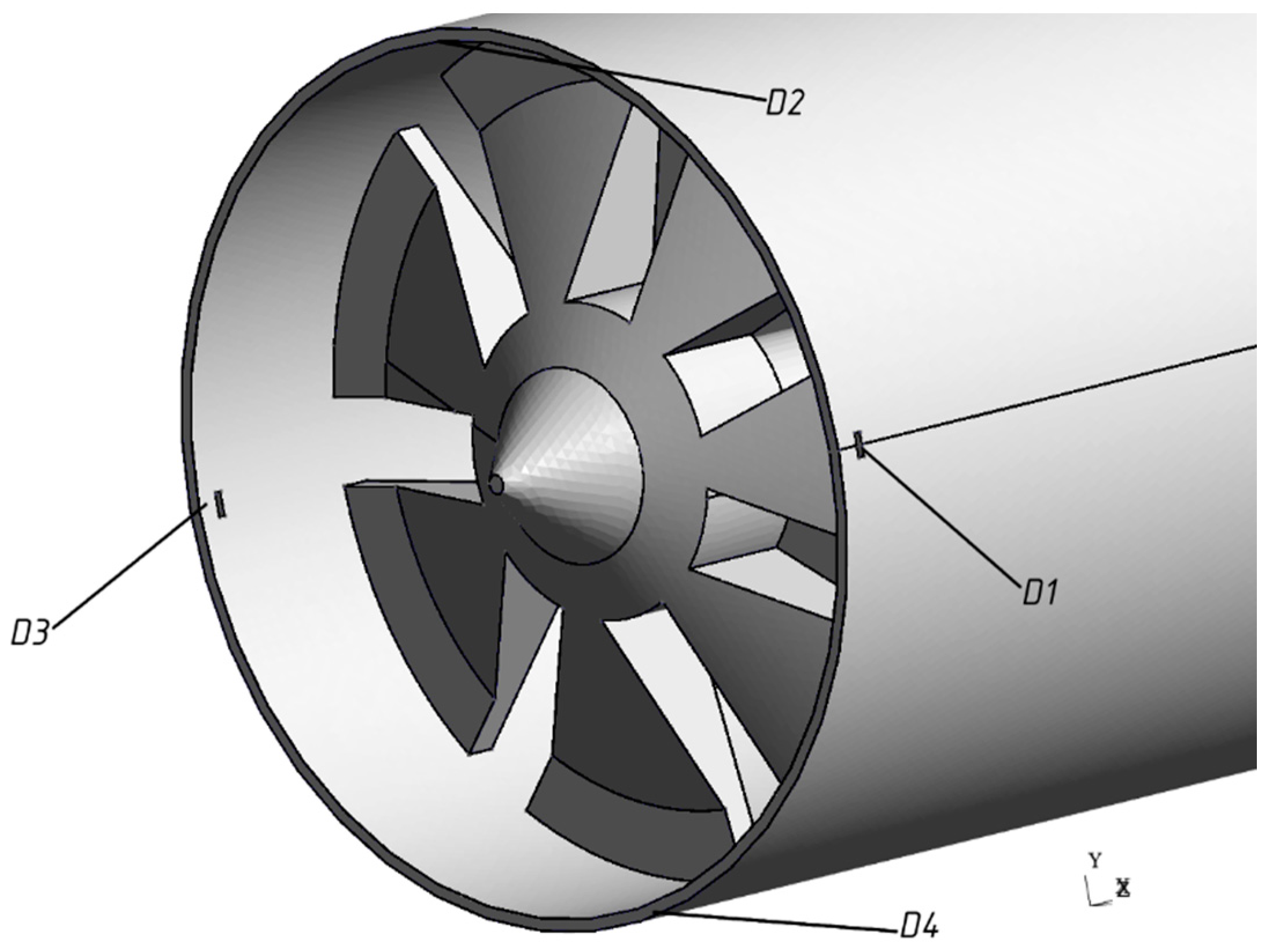
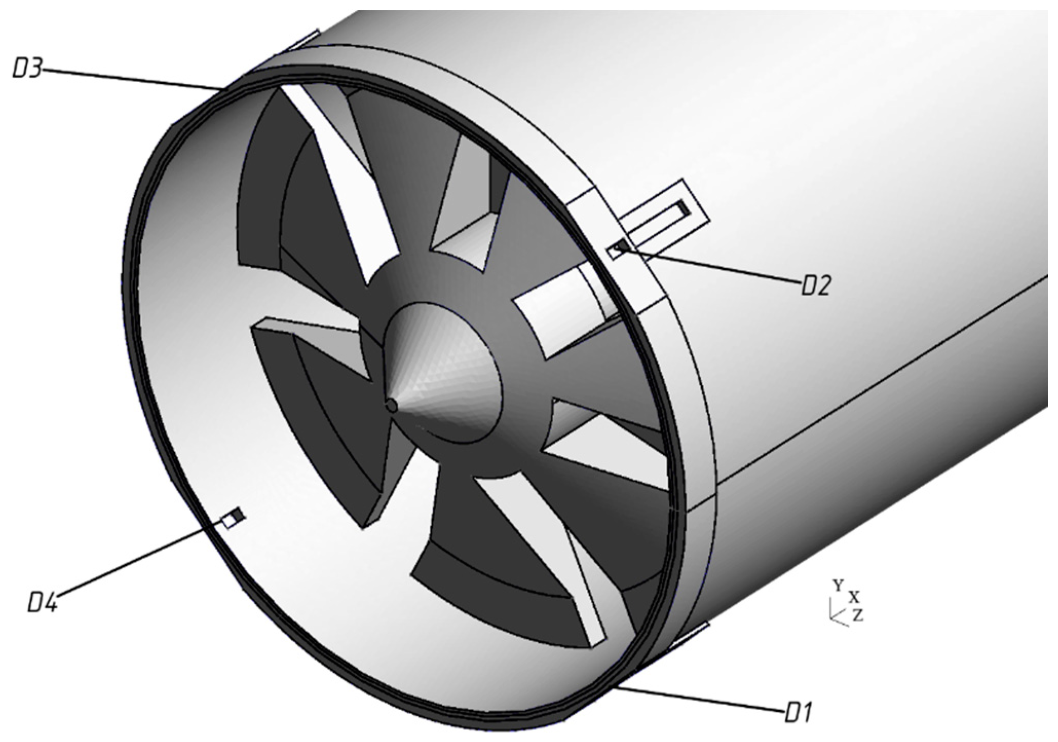
The arrangement of magneto-sensitive elements (the models are made as ferroprobe cores) is shown on the shield conventional geometric model (Figure 2) as positions “D1” ... ”D4”. “D1” and “D3” elements are arranged along the power cable axis direction and align with the tunneling shield. “D2” and “D4” elements are arranged in the plane perpendicular to the shield axis. It should be noted that there is no need to record the magnetic induction vector component normal to the shield housing surface as its value is close to zero.

4. Numerical Study of Magnetic Field Distribution

Numerical modeling of the magnetic field distribution pattern was performed for the following cases:

1. The power cable axis and tunneling shield longitudinal axis are in the same plane. The angle between axes varies within the range from 0 to 90 degrees.

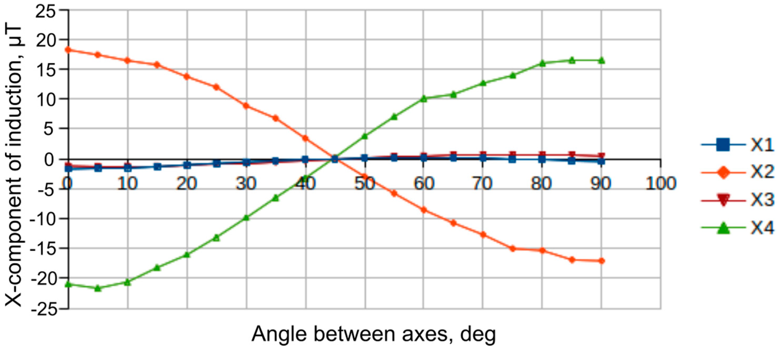
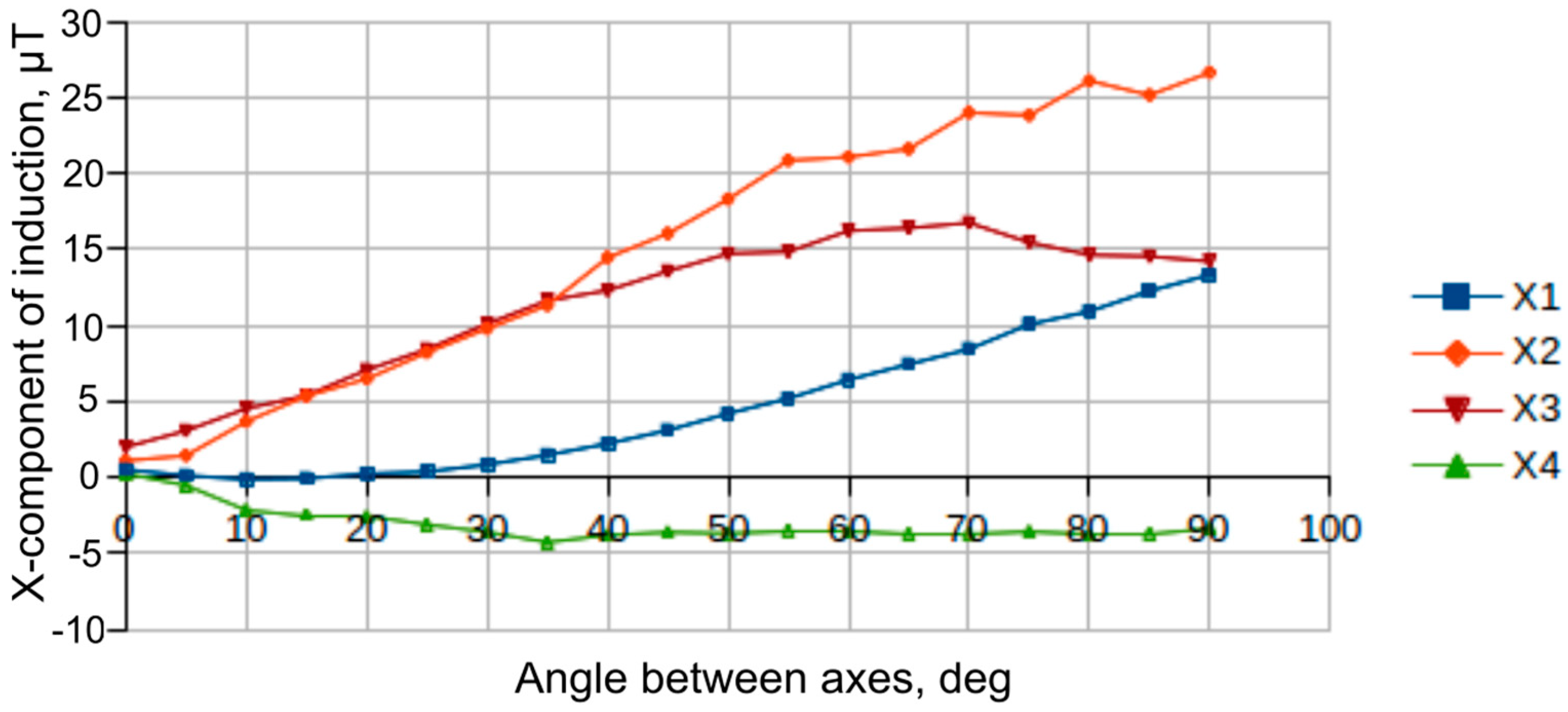
2. The tunneling shield longitudinal axis is offset parallel to the power cable axis. The angle between axes (with an offset between projections of the axes) varies within the range from 0 to 90 degrees. As the angle between the tunneling shield power cable and longitudinal axis changes (with their arrangement in the same plane), magnetic flows get redistributed between opposite (relative to the tunneling shield longitudinal axis) zones of D1–D3 and D2–D4 sensors. At the same time, the magnetic induction vector component, parallel to the tunneling shield longitudinal axis, recorded by “D2” and “D4” magneto-sensitive elements (hereinafter referred to as “X” component) changes when the angle between the power cable and the tunneling shield longitudinal axis changes within the range from 0 to 90 degrees proportionally with a change in sign, i.e., the magnetic flow changes direction at 45 degrees and reaches the maximum and minimum values at 0 and 90 degrees (Figure 3). The same components in zones of D1 and D3 sensors have the same sign and values, lower by order than in D2 and D4 zones.

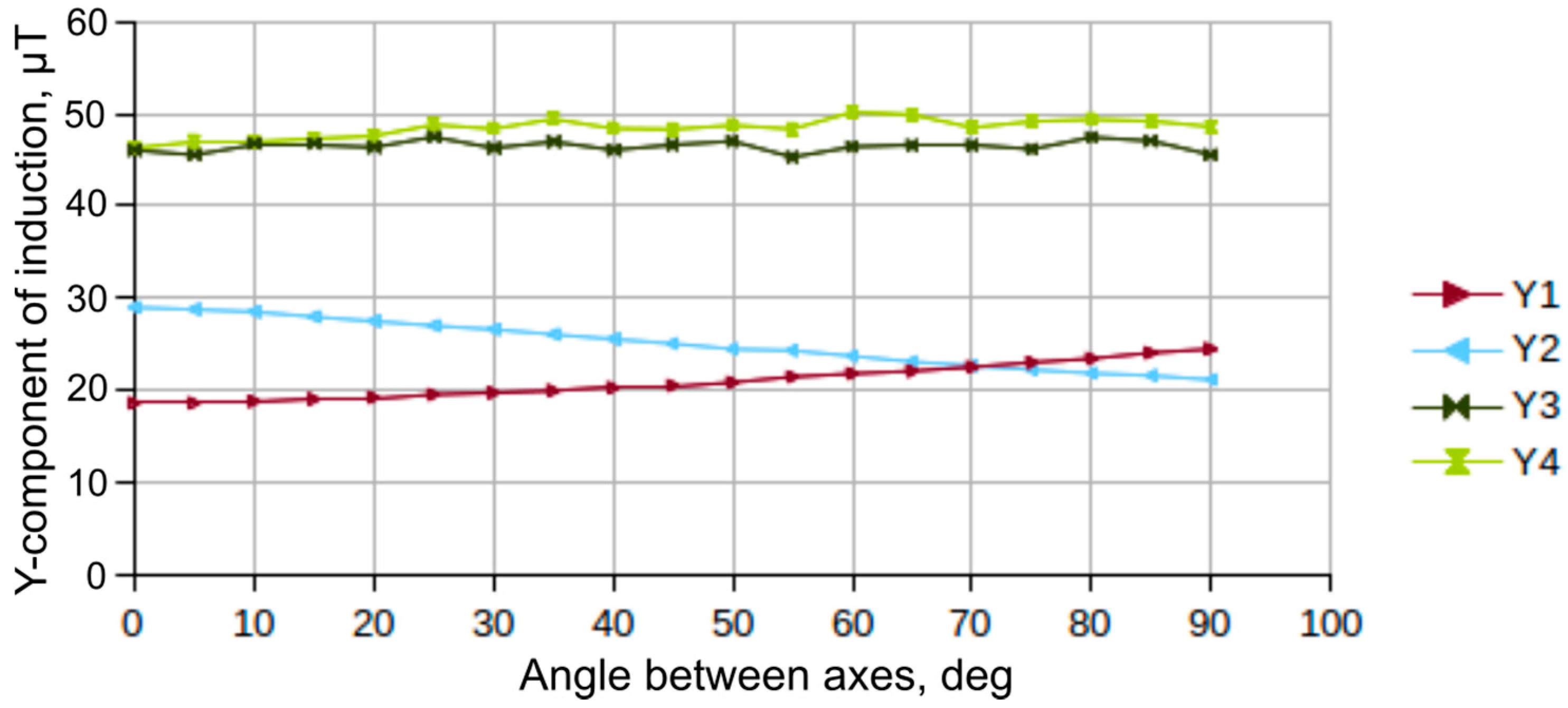
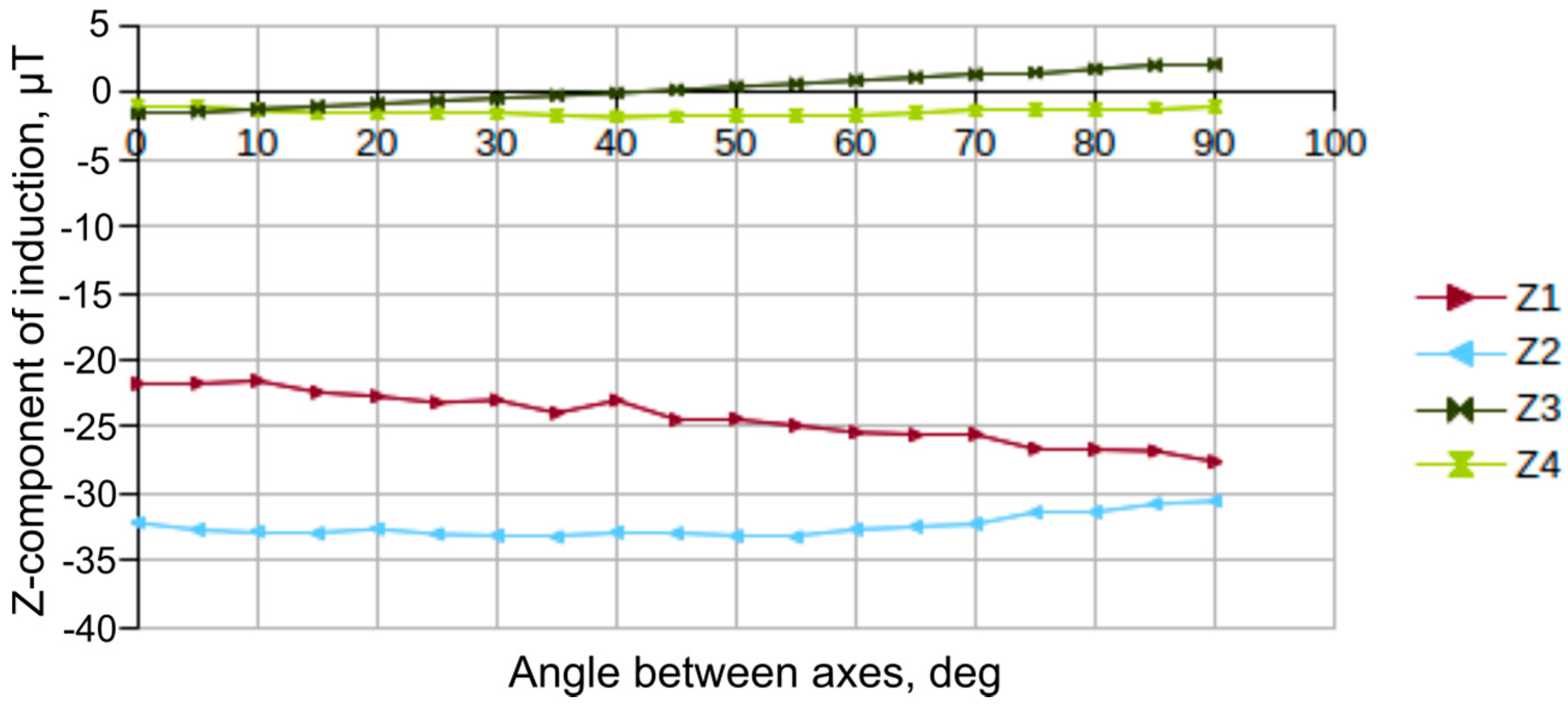
Components of the magnetic induction vector along the Z and Y axes vary depending on the angle between the tunneling shield longitudinal axis and power cable axis. The values of magnetic field induction components along the Y and Z axes, recorded by D3 and D4 elements, slightly increase with angle increase (Figure 4 and Figure 5, “Y3”, “Y4”, “Z3” and “Z4” dependences). The values of vector components recorded by the D1 and D2 elements remain nearly unchanged. In this case, values of the components along the D1 sensor Z-axis and D2 sensor Y-axis decrease, while the D2 element Z component and D1 element Y component increase.

In the case of the tunneling shield parallel displacement relative to the power cable, the type of dependences of the magnetic induction vector components on the angle between the tunneling shield longitudinal axis and power cable axis changes. Thus, when the tunnel shield is displaced by 1.5 m, the type of “X” component change becomes asymmetric for all magneto-sensitive elements (Figure 6).

Depending on the measure of the angle between the power cable and tunneling shield axes, the type of the dependence of magnetic induction vector components, recorded by magneto-sensitive elements on the value of tunneling shield parallel displacement also fundamentally changes [29]. In particular, for the “X” components of “D2” and “D4” elements (Figure 3), their sharp change is observed when the shield is displaced by an amount greater than its diameter with an increase in the angle between the power cable and tunnel shield axes to 45–90 degrees (Figure 7). If angle values are close to zero, values of the “X” component changes smoothly and proportionally to the offset value increase.

Considering mostly horizontal arrangement of power cables in the ground and above-stated type of the change in magnetic field topology for individual magneto-sensitive elements with the change of mutual position of the power cable and tunneling shield to ensure a significant change in the magnetic field topology in the area of all magneto-sensitive elements, it is recommended to change the arrangement of the ferroprobes by their turning relative to shield longitudinal axis by 45 degrees.

To continue relevant numerical studies, the following changes were made to the geometric model of the tunneling shield, consisting of the addition of the blade part with a cutting edge with grooves for ferroprobe sensors, oriented at 45 degrees to the plane, passing through the tunneling shield and power cable longitudinal axes. The grooves are made in the housing shell to accommodate measuring transducers of ferroprobe sensors. Transducer grooves are equipped with a safety stop to prevent damage to their contents by ground pressure. The modified geometric model of the blade part of the micro-tunnel-boring shield is shown in Figure 8.

The massive cutting edge acted as a magnetic flux concentrator, which led to its redistribution and increase in local magnetic flux density in the area of the ferroprobe location by 10–15% (Figure 9).

Based on the performed numerical modeling results, good symmetry and consistency of values of diametrically opposite sensors (for example, D1 and D3) for X and Z components (Figure 10 and Figure 11), as well as consistency of changes in the components along the Y-axis (Figure 12) for all sensors are observed.

As a result, it was determined that at 65 A current in a power electric cable, the values of magnetic induction vector components in ferroprobe cores reach the following values:

2–5 μT for the “X” component, 17−27 μT for “Y” and 3–14 μT for the “Z” component. With the electric current intensity of 5 A in the power cable, the values of the magnetic induction vector components in the ferroprobe cores go down to 55–620 nT, 1.1–3.0 μT and 0.1–6.0 μT for X, Y and Z components, respectively. The resulting values correspond to the measurement range of selected ferroprobes HB0391.5-20/3.

Thus, numerical modeling results show that the selected arrangement and orientation of ferroprobes make it possible to obtain magnetic induction values in the cores, corresponding to the measurement range of the ferroprobes with the change of mutual arrangement and orientation of the micro-tunnel-boring shield and electromagnetic field source—the power electric cable. Cumulatively, it provides detection of power cables of the packaged transformer substations from 20 kVA at the distance of at least 3 m from the shield front.

5. Experimental Study of Magnetic Field Distribution

The experimental facility model (Figure 13) includes the following: a steel tube with a diameter of 1400 mm, imitating the micro-tunnel-boring shield, with four mounted measuring modules with ferroprobes (HB0391.5–35 ferroprobe model) and the regulated current supply (powerful laboratory power supply of ABB company). The measuring modules are connected to a laptop via an RS485-USB converter. The tested cable was located on the wooden chassis and connected to the adjustable current source. The power cable of VBbShv type 3 × 16(ozh)–6 was used for the test. The cable section was defined by the maximal current set at the tests. Ferroprobes placed into installation notches of the tube imitating the tunnel shield are equipped with bias windings for calibration and initial installation of the probes.

The cable chassis with the 4-wire armored cable fixed on its movable bar, connected to the current source, was located at a distance of 3 m from the tube. The cable conductors are connected in parallel two-by-two. At one of the cable ends, the conductors are closed to imitate the real power cable connected to the load. The current in the cable was changed stepwise. The value of current provided by the source was changed in the range from 0 to 300 A. At this, ferroprobe was adjusted to maximal sensitivity—200 mV per μT. The largest signal change was obtained at the Z-axis. For the setting of zero values of induction components, the respective current values were set in the bias windings. 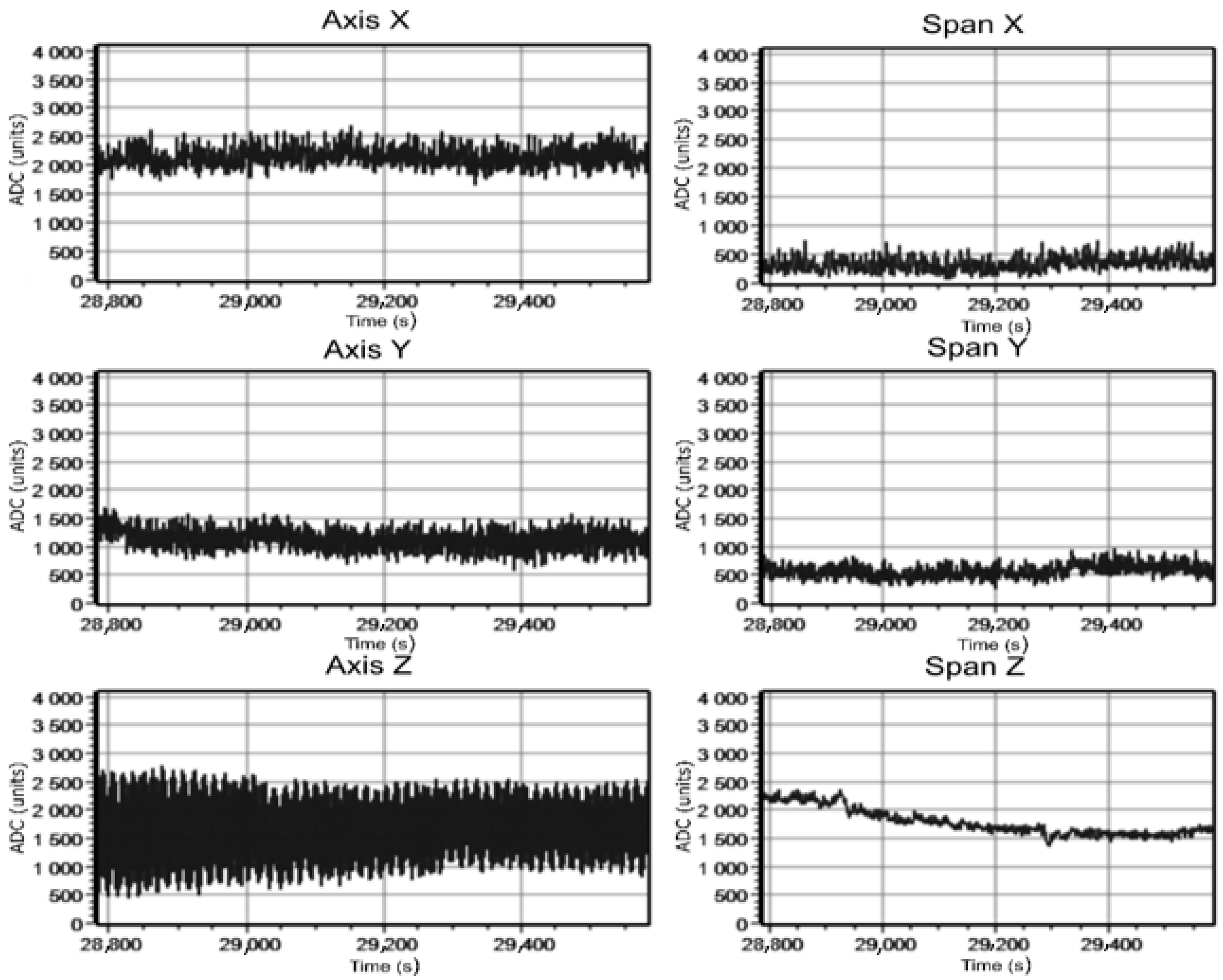Figure 14 and Figure 15 represent oscillograms of the output signals of the different channels of the ferroprobe measuring module. The data were obtained for different amplification gain factors of the ferroprobe measuring module and values of the current in the cable. Graphs on the left show the output signals of the ferroprobe measurement module, taken from microcontroller ADC channels, corresponding to magnetic field induction components (three axes). The distinct signal change at the Z-axis is seen from the graphs, which gives the possibility to assess the magnetic field created by the current in the cable. Signal change at the Y-axis is less notable, which is connected with the cable positioning in relation to the probe. Graphs on the right represent dependences of signal differences by axes between the maximal and the minimal values in the AD converter units. Based on the graphs, we can conclude that when the cable is arranged perpendicular to the sensor axis, the most informative indicator of the live conductor presence is a signal from the channel corresponding to the Z-axis, where a weak external source of the magnetic field, recorded by the ferroprobe, is most obviously represented, confirming numerical modeling results. From graphs in Figure 15, it is seen that at high gain, the signal value along the Z-axis exceeds the set level at high currents, associated with the microcontroller’s ADC resolution. The measured values of the Z-component of the magnetic field induction were 72 nT at a current of 65 A and 330 nT at a current of 295 A. The X-and Y-components had a near-zero value at a current of 65 A. At a current of 295 A, these components had a value of 45 and 100 nT.

In the considered case, the currents in the biasing windings of the ferroprobe were 9.4, 54 and 13 mA (X, Y and Z channels). This is equal to 374, 2200 and 505 ADC units (for gain ratio 128).

Figure 16, Figure 17 and Figure 18 show oscillograms of sensor signals without current and for current in cables 65 A and 295 A in ADC units versus time in milliseconds. Similar to the previous experiment, the cable was located horizontally at the shield axis height and at the distance of 3 m to its frontal section. Graphs on the left show the probe signals in the microcontroller AD converter codes at three axes for the period. The period is represented by the distance between two perpendicular lines on the graph. The oscillograph recordings on the right demonstrate the signal differences at three axes in the AD converter units vs. time in ms. Figure 16 shows that the probe records the weak sinewave component signal at the absent current in the cable. It is connected with the presence of power lines located at a certain distance of one hundred m from the experiment site. Graphs in Figure 17 and Figure 18 show the situation when the cable is connected to a voltage source with a distinct sinusoidal signal at the sensor output along the Z-axis, different in amplitude depending on the current value. On other axes, the signal is not so clear due to cable orientation. With the purpose to detect the cable position in relation to the tunnel shield, the following two experiments were conducted.

The first experiment was to move the cable vertically. In the course of the second experiment, the cable was rotated in relation to the shield axis. Measurements were carried out at the cable current of 65 A and 295 A at 3 m distance to the shield frontal section. Oscillograph recordings of magnetic induction signals in the AD converter codes for the first experiment are given in Figure 19 and Figure 20.

Graphs in Figure 19 and Figure 20 show that when the cable is moved vertically, the signal along all axes most clearly changes along the Z-axis. It confirms the possibility of recording the test cable magnetic field at its position change. The maximum value change of the output signal magnitude for this field component was 415 nT (“span” graph, the difference between the maximum and minimum value) for 295 A current value. The results of changing signals for the second experiment connected with the cable rotation in the plane perpendicular to the tube axis demonstrate the slight change in the magnetic induction signal value, but its detection is possible (Figure 21 and Figure 22). In this case, the value change of the output signal magnitude for the Z-component was 214 nT and 14 nT for the Y-component (295 A current value).

6. Conclusions

The results of numerical simulation of a three-dimensional magnetic field of a current-carrying conductor and a micro-tunnel-boring shield indicate the possibility of using the magnetometric method for detecting power cable lines. Ferroprobes can be placed in the housing of the micro-tunnel-boring shield. Based on the results of the study of changes in the topology of the magnetic field with a change in the relative position of the power cable and the orientation of the tunnel shield, the locations of the sensors were selected. It was found that the measurement of the components of the magnetic induction vector through three measuring channels of the sensor with a change in the relative position and orientation of the micro-tunnel-boring shield and cable with a current of 60–70 A and more theoretically provides the possibility of detecting power cable lines from standard complete transformer substations with a capacity of more than 20 kVA at a distance of 3 m from the cutting edge of the micro-tunnel-boring shield.

The results of numerical simulation were confirmed by experimental studies on a full-size dummy of a micro-tunnel-boring shield. It was found that the most informative is the output signal of the sensor channel, which registers the magnetic field vector component that coincides with the longitudinal axis of the micro-tunnel-boring shield (Z). The significant influence of parasitic noise caused by external magnetic fields (natural magnetic background and background magnetic field of industrial zones and urban territories) and high sensitivity of the ferroprobes requires the use of additional filters, and therefore with the help of biasing windings, it is possible to compensate only the constant component of external magnetic fields. At currents of more than 200 A, it becomes possible to determine the position of the cable by the output signal from the X and Y channels of the ferroprobes. Thus, the results of the experiments confirm the possibility of practical implementation of the magnetometric sensing system for installation in the housing of the micro-tunnel-boring shield.