Article

Adaptive Population NSGA-III with Dual Control Strategy for Flexible Job Shop Scheduling Problem with the Consideration of Energy Consumption and Weight

1
Intelligent Electrical Science and Technology Research Institute, Northeastern University, Shenyang 110819, China
2
Key Laboratory of Integrated Energy Optimization and Secure Operation of Liaoning Province, Northeastern University, Shenyang 110819, China
3
Shenzhen Institute of Advanced Technology, Chinese Academy of Sciences, Shenzhen 518055, China
4
Shenyang Institute of Automation, Chinese Academy of Sciences, Shenyang 110169, China
*
Author to whom correspondence should be addressed.
Machines 2021, 9(12), 344; https://doi.org/10.3390/machines9120344
Submission received: 11 November 2021 / Revised: 23 November 2021 / Accepted: 1 December 2021 / Published: 9 December 2021
(This article belongs to the Topic Robotics and Automation in Smart Manufacturing Systems)

Abstract

:
The flexible job shop scheduling problem has always been the focus of research in the manufacturing field. However, most of the previous studies focused more on efficiency and ignored energy consumption. Energy, especially non-renewable energy, is an essential factor affecting the sustainable development of a country. To this end, this paper designs a flexible job shop scheduling problem model with energy consideration more in line with the production field. Except for the processing stage, the energy consumption of the transport, set up, unload, and idle stage are also included in our model. The weight property of jobs is also considered in our model. The heavier the job, the more energy it consumes during the transport, set up, and unload stage. Meanwhile, this paper invents an adaptive population non-dominated sorting genetic algorithm III (APNSGA-III) that combines the dual control strategy with the non-dominated sorting genetic algorithm III (NSGA-III) to solve our flexible job shop scheduling problem model. Four flexible job shop scheduling problem instances are formulated to examine the performance of our algorithm. The results achieved by the APNSGA-III method are compared with five classic multi-objective optimization algorithms. The results show that our proposed algorithm is efficient and powerful when dealing with the multi-objective flexible job shop scheduling problem model that includes energy consumption.

1. Introduction

Facing the global competition of the integration of the world economy, if the manufacturing industry wants to stand out from the cruel survival of the fittest, it must accelerate its response to external changes, improve product quality and performance, reduce various costs in the process, and provide customer-based personalized service on-demand [1,2]. At the same time, affected by the deterioration of the climate and the greenhouse effect, society and the country have also put forward higher and higher requirements for the green production of enterprises [3,4]. The manufacturing industry, which accounts for half of the total carbon emissions, has also attracted the attention of society and governments at all levels [5,6]. Therefore, ensuring a high-efficiency production rhythm in production and processing while seeking to improve energy efficiency and reduce total carbon emissions has become the direction of the study efforts of experts and scholars [7,8].
The manufacturing industry plays an indispensable role in the economic development and social construction of a country [9,10]. At the same time, the manufacturing industry is also an area where a country invests a tremendous amount of energy consumption [11,12]. According to the international energy outlook 2021 reference case, after a period of decline in coal consumption through 2030, consumption of all major fuels will grow from 2030 to 2050. Renewable energy consumption will more than double between 2020 and 2050, and renewable energy consumption will nearly equal liquid fuels consumption by 2050 [13]. In China, manufacturing companies consumed more than 50% of the national electrical energy and generated at least 26% of the total carbon dioxide emission. As the primary industry of the national economy, the manufacturing industry plays a crucial role in developing the national economy [14,15]. Still, it is also the main body of energy consumption and environmental pollution [16,17]. Promoting energy conservation and emission reduction in the manufacturing industry is of great significance to the global implementation of green manufacturing and actively responding to challenges such as global warming [18].
With the development of science and technology, the production scale and complexity of the manufacturing industry are getting higher and higher [19,20]. As a necessary means to solve the resource arrangement, flexible job shop scheduling problem (FJSP) plays an increasingly important position in the production and operation activities of the manufacturing industry [21,22]. FJSP refers to the process of making full use of the limited resources of the enterprise through reasonable allocation to meet or optimize one or more goals [23,24]. The FJSP is an essential part of the manufacturing process of the entire production job shop and controls the entire manufacturing system [25,26,27]. A reasonable scheduling plan can reduce the production cost of the enterprise, shorten the production cycle, improve the enterprise’s competitiveness, and bring significant economic benefits to the enterprise [1,28]. With the advancement of green manufacturing, FJSP that considers energy saving and consumption reduction goals are essential for companies to achieve low-carbon development models [29,30].
Mouzon et al. devised a mathematical programming model for optimizing the scheduling problem of a single computerized numerical control (CNC) machine that considered the energy consumption and total completion time [31]. Afterward, Lei et al. deemed an energy-related objective should be considered thoroughly in FJSP with the advent of green manufacturing and proposed an FJSP with the consideration of energy consumption [32]. Additionally, to minimize makespan and total tardiness under the constraint that total energy consumption does not exceed a given threshold, a multi-objective FJSP with an energy consumption threshold is formulated by Wang et al. [29]. Jiang et al. established the mathematical model of the low-carbon FJSP with the objective of minimizing the sum of the energy consumption cost, and the earliness/tardiness cost. In another work, Meng et al. modeled the mixed integer linear programming (MILP) models for FJSP with the objective of minimizing total energy consumption [23].
However, research on reducing the energy consumption of manufacturing processes has concentrated chiefly on the machine, product, and production management levels [29]. There is much necessary energy consumption that has not been considered in previous studies [33]. Especially for small and medium-sized enterprises with small processing scales, improving processing efficiency is their first focus. With the continuous progress of the industrialization process, establishing an efficient scheduling model that contains more detailed energy consumption is an inevitable trend of development [2]. In this case, some minor energy consumption considerations become particularly important for saving costs and preventing environmental pollution [34]. For this reason, this paper considers various energy consumption components in the manufacturing industry that have not been considered in many previous studies but cannot be ignored, and designs the multi-objective FJSP considering the energy consumption of the transport, set up, processing, unload, and idle phase. Meanwhile, this paper also considers the weight property of the bars. The heavier the bar, the more energy will be consumed.
A variety of multi-objective optimization algorithms have been proposed in many studies [35]. For multi-objective FJSP, Gao et al. combined the particle swarm algorithm and tabu search algorithm and proposed an effective hybrid algorithm to solve multi-objective FJSP with several conflicting and incommensurable objectives [36]. In another study, Gao et al. proposed a discrete harmony search algorithm for FJSP with minimization of multiple objective functions of the maximum of the completion time and the mean of earliness and tardiness [37]. Moreover, Li et al. proposed an effective hybrid tabu search algorithm (HTSA) to solve the FJSP with three minimization objectives of the maximum completion time (makespan), the total workload of machines, and the workload of the critical machine [38]. Lu et al. formulated the FJSP mathematical model with the objectives of minimizing both the makespan and the total additional resource consumption [39].
Most of the research has achieved excellent results for their issue. However, for FJSP as an NP-hard problem, the solution space will exponentially increase with jobs and operations [40,41,42]. Meanwhile, FJSP is a discrete problem; many algorithms that are good at dealing with continuous problems are not suitable for solving FJSP [43,44]. Many algorithms and improvement strategies are challenging to achieve a satisfactory effect for it [45,46]. The genetic algorithm (GA) is a very suitable tool for solving combinatorial optimization problems, such as FJSP. The non-dominated sorting genetic algorithm III (NSGA-III) algorithm is an extension of the GA in multi-objective optimization, which has been applied to various practical fields, so this paper adopts NSGA-III as a basic algorithm when solving FJSP. In order to further improve the solution ability of NSGA-III to prevent it from falling into the local optimum, and to enhance the diversity of the population, this paper proposes a dual control strategy (DCS) for multi-objective optimization and combines it with NSGA-III to avoid precocity and enhance the optimization capability of NSGA-III on solving combinatorial optimization problems such as FJSP. The highlights of this paper are as follows:
(1) The FJSP model considering energy consumption that covers the transport of AGV and set up, processing, unload, and idle of the machine is designed.
(2) The weight attribute of the bars is also taken into account. The heavier the bar, the more energy it consumes.
(3) The DCS for multi-objective optimization is formulated to enhance the solving ability of NSGA-III.
The rest of this work is arranged as follows. Firstly, the details of FJSP are elaborated in Section 2. Then, the procedure of the adaptive population non-dominated sorting genetic algorithm III (APNSGA-III) is described in Section 3. Followed by the extensive experiments that are conducted in Section 4. Finally, we summarize the paper in Section 5.

2. Problem Description

Classic FJSP can be described as: there are n jobs J = ( J 1 , J 2 , , J n ) that are processed on m machines M = ( M 1 , M 2 , , M m ) in a production job shop. Each job J i consists of n i operation, O i , j denotes the j t h operation of the i t h job. Each operation can be processed on any machine that belongs to machine set M i , j . There are the following assumptions (constraints) about the FJSP [47].
(1) The completion time of the j t h operation of the i t h job is the sum of its start time and processing time.
C i j k = S i j k + T i j k
where C i j k , S i j k , T i j k implies the completion time, the starting time, and the processing time of the j t h operation of the i t h job on machine M k , respectively.
(2) The start time of the j t h operation of the i t h job on the machine M k is determined by the completion time of the previous operation q on the machine and the completion time of the previous operation of the job.
S i j k = m a x { S ( i 1 ) q k + T ( i 1 ) q k , C i ( j 1 ) ( k 1 ) }
(3) The downtime of machine M k is the completion time of the last operation on the machine.
C T k = C l k
where l represents the last job on machine M k , C l k indicates the completion time of the last job on machine M k .
(4) There are constraints on the machine required for the processing operation.
C g k C i k + M ( 1 x i g k ) T g k , i , g = 1 , 2 , , n ; k = 1 , 2 , , m
where n and m denotes the number of jobs and machines, respectively. C g k , T g k indicates the completion time and processing time of job J g on machine M k , M means a sufficiently large positive number. x i g k represents the processing priority of job J i and job J g on machine M k . If the job J i is processed first, then x i g k is 1, otherwise it is zero.
(5) Operation O i j and O g z cannot be processed on any machine on machine set M i j M g z at the same time.
S i j k C g z k Z i j g z k M , k M i j M g z
S g z k C i j k ( 1 Z i j g z k ) M , k M i j M g z
where Z i j g z k represents that operation O i j is processed before operation O g z on machine M k , 1 if yes, 0 otherwise. M i j M g z denotes the machine set that can process operation O i j and operation O g z at the same time.
(6) There is a priority relationship between the various operations of the same job.
S i j k C i ( j 1 ) k , k M i j , i = 1 , 2 , . . . , n , j = 2 , . . . , K i
where K i represents the number of operation of job J i .
(7) All jobs can be processed and all machines are optional when a task starts.
S i j k 0
C i j k 0
(8) Only one machine can be selected for each operation.
k = 1 m R i j k = 1
where R i j k denotes whether the machine M k processes operation O i j , 1 means processed, 0 means unprocessed.
This paper considers two optimization objectives in the FJSP model that include the maximum completion time and the total energy consumption.

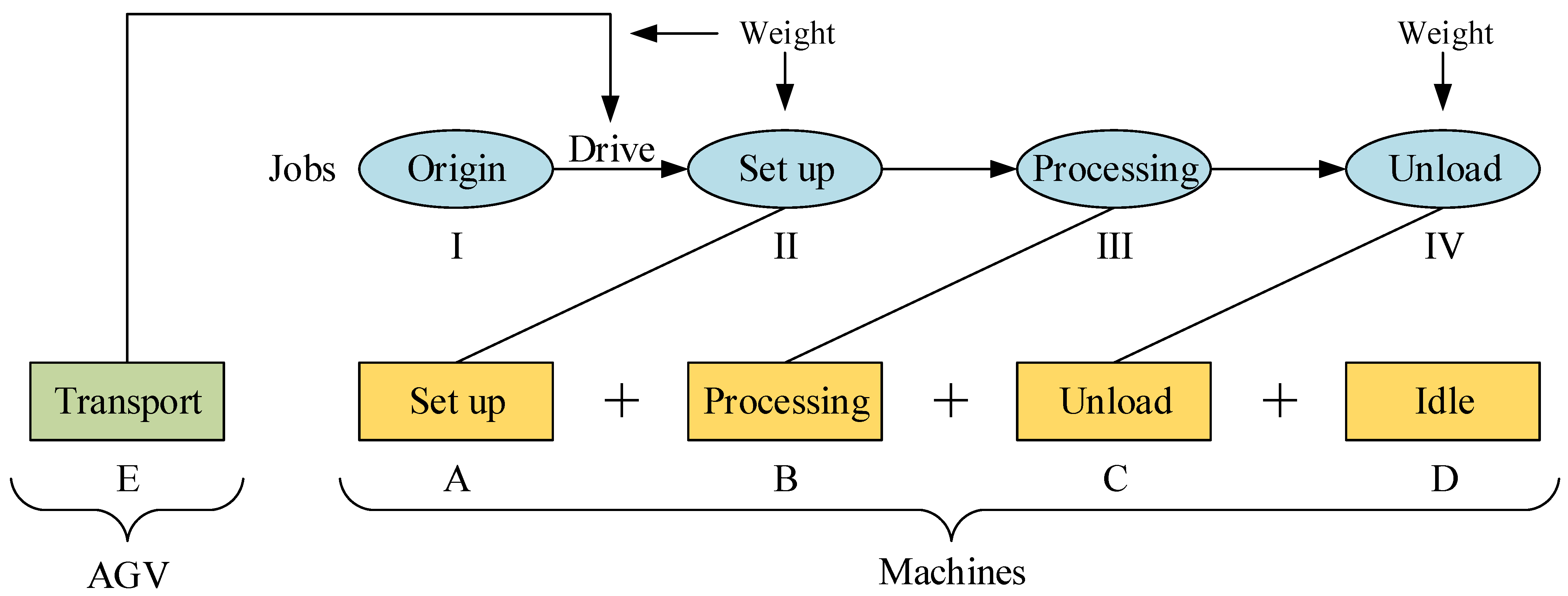
2.1. Maximum Completion Time (Makespan)

f 1 = m i n ( M a k e s p a n ) = m i n m a x 1 k m m a x 1 i n C T k
where M a k e s p a n represents the maximum completion time of all machines, it is the main indicator to measure the completion time of all jobs. C T k is expressed as:
C T k = i = 1 n j = 1 K i ( S i j k R i j k + R i j k T i j k )
where R i j k denotes whether the machine M k processes operation O i j , 1 means processed, 0 means unprocessed.

2.2. Total Energy Consumption (TEC)

The total energy consumption considered in this paper is mainly composed of the following five parts.
(a): The transporting energy consumption ( T T E C )
T T E C is the energy consumed by the AGV transporting the job between machines. T T E C is related to the time AGV takes to transport the job and the weight of the job. It can be calculated by the following equation.
T T E C = i = 1 n j = 1 K i T i j W i P
where T i j implies the time spent in transporting the job J i at the j t h operation, W i means the weight of the job J i . P represents the energy consumed to transport a kilogram of objects per second.
(b): Total set up energy consumption ( T S E C )
T S E C is the energy consumed by the machine to grab the job and set it on the processing table. Different operations of different jobs have different set up energy consumptions on different machines. Moreover, T S E C is positively related to the weight of the bar; the heavier the bar, the more energy it consumes. It can be calculated by the following equation.
T S E C = i = 1 n j = 1 K i k = 1 m S i j k R i j k W i
where S i j k represents the energy consumption per unit weight for machine M k to set up O i j , W i denotes the weight of the job J i .
(c): Total processing energy consumption ( T P E C )
T P E C is the main energy consumption that is used to perform operations such as punching, cutting, laser printing, spray painting, etc. Different operations of different jobs have different processing energy consumptions on different machines. The calculation of T P E C is not given in Equation (15).
T P E C = i = 1 n j = 1 K i k = 1 m E i j k R i j k
where E i j k means the energy consumed by machine M k processing operation O i j , R i j k indicate whether the j t h operation of the i t h job is processed on machine M k , 1 if yes, 0 otherwise.
(d): Total unloading energy consumption ( T U E C )
Corresponding to T S E C , T U E C is the energy consumed by the unloading job by machine. Different operations of different jobs have different unload energy consumptions on different machines. Moreover, T U E C is positively related to the weight of the bar; the heavier the bar, the more energy it consumes. It can be calculated by the following equation.
T U E C = i = 1 n j = 1 K i k = 1 m U i j k R i j k W i
where U i j k represents the energy consumption per unit weight for machine M k to unload processing operation O i j , W i denotes the weight of the job J i .
(e): Total idling energy consumption ( T I E C )
The machine in the job shop still consumes energy when it is not working, T I E C is the energy consumed when the machine is idle. Different machines consume different energy in standby state. It is given by following Equation (17).
T I E C = i = 1 m N i C i
where N i denotes the total idle time of machine M i , C i represents the energy consumption per minute when the machine is idle, m implies the number of machines.
Therefore, the second optimization objective T E C can be formulated as follows:
f 2 = m i n ( T E C ) = m i n ( T P E C + T T E C + T S E C + T U E C + T I E C ) = m i n ( i = 1 n j = 1 K i T i j W i P + i = 1 n j = 1 K i k = 1 m S i j k R i j k W i + i = 1 n j = 1 K i k = 1 m E i j k R i j k + i = 1 n j = 1 K i k = 1 m U i j k R i j k W i + i = 1 m N i C i )
Figure 1 shows the main structure of our FJSP model. Each job needs to go through I–IV statuses from raw material to finished product, namely, origin, set up, processing, and unload. Each machine has A–D functions, namely, set up, processing, unload, and idle. Automatic guided vehicle (AGV) has only one E function, which is to transport jobs. Status I to status II of the jobs need to be driven by AGV, and the energy consumed by this part will also be recorded in the total energy consumption, which is the transportation consumption. Status II–IV of one job needs to be implemented by one machine’s A–C functions. Notably, the weight attribute of jobs is considered in the transport, set up, and unload stages. The heavier the bars, the more energy is consumed in these three stages. The processing stage of the job does not consider the weight attribute because in our model, we assume that the job is placed on the processing table at this stage, and there is no need to overcome gravity to do work. The machine is idle when it is not processing any jobs. Therefore, the total energy consumption of the workshop can be attributed to the sum of the energy consumption of the AGV transporting the job and the energy consumption of the four functions of the machine.
To more vividly illustrate the details of energy consumption information mentioned before, we place the Gantt chart of the 3 × 3 scale FJSP into Figure 2. At the beginning of the task, the time for the job to reach the machine through transport will also be recorded in the scheduling. The job must go through the set up stage before being processed. After the operation of the job is processed, it must go through the unload stage. A machine can only perform one of the set up, process, and unload stages on operations simultaneously. The transporting has nothing to do with any operation of the machine and it is related to AGV that is robot dedicated to transporting workpieces. As long as the job is finished performing the unload operation, it will be boxed and transported off the production line. Moreover, the job can be queued to be processed, as long as the unloading of the previous job on the machine is completed, and the setup stage can be carried out immediately.
We can find that the idle time of the machine occupies a large proportion of the scheduling. It once again highlights the importance of investigating the energy consumption of the machine without a load.
An instance of the FJSP is given in Table 1. As it can be observed, there are three jobs to be processed on three machines. Job J 1 , J 2 , J 3 , all have three operations. The information of (set up time/ set up energy consumption), (processing time/process energy consumption), (unload time/unload energy consumption) are shown in Table 1. For instance, the available machines of the O 11 are machine M 2 and machine M 3 . The processing time of O 11 on machine M 2 and machine M 3 is 40 min and 46 min, respectively, while the set up energy consumption of O 11 on machine M 2 and machine M 3 is 46 kWh and 65 kWh, respectively. The set up time of O 11 on machine M 2 and machine M 3 is 9 min and 7 min, respectively, while the set up energy consumption of O 11 on machine M 2 and machine M 3 both are 21 kWh. The unload time of O 11 on machine M 2 and machine M 3 is 2 min and 8 min, respectively, while the set up energy consumption of O 11 on machine M 2 and machine M 3 is 11 kWh and 16 kWh, respectively. After completing the preceding operation of a job on a machine tool, the AGV will convey the job from the current machine to another machine. The transportation time between different machines is shown in Table 2.

3. Improved NSGA-III

NSGA-III is the extension of the NSGA-II. NSGA-III and NSGA-II have a similar framework. The difference between the two is mainly the change in the selection mechanism. NSGA-II primarily relies on the crowding degree for sorting, and its role in high-dimensional target space is not prominent, while NSGA-III has drastically adapted the crowding degree sorting. Maintain the diversity of the population by introducing widely distributed reference points. The individual selection mechanism of NSGA-III is shown as follows.

3.1. Non-Dominated Sorting

Suppose the individual number of the current population P t is N, that is | P t | = N . Generate Q t through genetic operator, that is | Q t | = N . The parent and child populations are combined as R t = P t Q t . Sort R t non-dominated and divide it into multiple non-dominated levels ( F 1 , F 2 , ) . Put the population members of the non-dominated level 1 to l into | S t | in turn. If | S t | = N , P t + 1 = S t . If | S t | > N , then part of the next generation is P t + 1 = i = 1 l 1 F i , the remaining individuals are selected in F l . The detailed selection procedure will be expanded in the following subsection.

3.2. Determination of Reference Points on a Hyperplane

The reference points of NSGA-III can be generated by a structured manner or supplied preferentially by the user. There are a variety of popular reference point preset methods; we introduce two popular methods.
Das and Dennis’s systematic approach: The reference point is on a ( M 1 ) -dimensional hyperplane, and M is the dimension of the target space. If we divide each target into H parts, then the number of reference points is:
P = m + H 1 H
For a three-objective problem with H = 4 , the reference points form a triangle and 15 reference points are generated according to formula (20).
The coordinates of each reference point are generated by the following rules:
(1): Let X be all the (M-1) combinations of 0 H , 0 H , , H + M 2 H ;
(2): For each x i j X , x i j = x i j j 1 H ;
(3): Let S be the reference point set, for each s i j S and x i j X ,
s i j = x i j 0 , j = 1 s i j = x i j x i ( j 1 ) , 1 < j < M s i j = 1 x i ( j 1 ) j = M
Deb and Jain’s method: It is suggested to use two layers of reference points, which are generated as follows [48]:
(1): Generate S 1 by Das and Dennis’s method as the point set on the boundary layer;
(2): Let S 2 be the point set on the inside layer, for each S i i S 2 and s i j S 1 ,
S i i = 1 2 s i j + 1 2 M ;
(3): The reference point set S = S 1 S 2 .

3.3. Adaptive Normalization of Population Individuals

First, the ideal point of the population S t is determined by identifying the minimum value z i m i n for each objective function i = 1 , 2 , , M by constructing the ideal point z ¯ = ( z 1 m i n , z 2 m i n , , z M m i n ) . Compute each dimension of the ideal point by z j m i n = m i n s S t f j ( s ) , and translate the objective by f j ( s ) = f j ( s ) z j m i n . Then, find the extra points corresponding to each coordinate axis using (22) and (23).
A S F = ( x , w ) = m a x i = 1 M f i ( x ) / w i , x S t
z i , m a x = s : a r g m i n s S t A S F ( s , w i ) , w i = ( τ , . , τ ) , τ = 10 6 , w j i = 1
For the i t h translate objective f i , generate an additional objective vector z i , m a x . M additional objective vectors will form an M-dimensional linear hyperplane. Find the intercept a i , i = 1 , 2 , , M . Then, the objective function can be normalized to:
f i n ( x ) = f i ( x ) / ( a i z i m i n ) = ( f i ( x ) z i m i n ) / ( a i z i m i n ) , i = 1 , 2 , , M
where the function value of the intersection of the normalized plane and the coordinate axis f i = 1 , the points on this normalized hyperplane satisfy i = 1 M f i n = 1 .

3.4. Link the Individuals to the Reference Points

After normalizing each objective adaptively based on the extent of members of S t in the objective space, it needs to associate each population member with a reference point. For this purpose, NSGA-III defines a reference line corresponding to each reference point on the hyperplane by joining the reference point with the origin. Then, calculate the perpendicular distance of each population member of S t from each of the reference lines. The reference point whose reference line is closest to a population member in the normalized objective space is considered to be associated with the population member.

3.5. Select Individuals

It is worth noting that a reference point may have one or more population members associated with it or need not have any population member associated with it. NSGA-III counts the number of population members from P t + 1 = S t / F l that are associated with each reference point. Denote this niche count as ρ j for the j t h reference point. NSGA-III devises a new niche-preserving operation as follows. First, identify the reference point set J m i n = { j : a r g m i n j ρ j } having minimum ρ j . In the case of multiple such reference points, one ( j ¯ J m i n ) is chosen at random.
If ρ j ¯ = 0 (meaning that there is no associated P t + 1 member to the reference point j ¯ ), there can be two scenarios with j ¯ in set F l . First, there exists one or more members in front F l that are associated with the reference point j ¯ . In this case, the one having the shortest perpendicular distance from the reference line is added to P t + 1 . The count ρ j ¯ for reference point j ¯ is then incremented by one. Second, the front F l does not have any member associated with the reference point j ¯ . In this case, the reference point is excluded from further consideration for the current generation.
In the event of ρ j ¯ 0 (meaning that one member associated with the reference point already exists in S t / F l ), a randomly 2 chosen member, if it exists, from front F l that is associated with the reference point j ¯ is added to P t + 1 . The count ρ j ¯ is then incremented by one. After niche counts are updated, the procedure is repeated for a total of K times to fill all of the vacant population slots of P t + 1 .

3.6. The Framework of APNSGA-III

In the selection operator of ordinary GA, solutions with lower fitness will always be eliminated. Sometimes inferior individuals also have a probability of becoming a superior solution. Frequent elimination of them will not only waste resources but also reduce randomness and reduce global search capabilities. To this end, this paper designs a DCS for multi-objective optimization to enhance the performance of the NSGA-III.
The details of the APNSGA-III are shown in Algorithm 1 and Figure 3. First, p o p that represents the entire population, b e s t that is the best solution found so far, B e s t _ n o t E n h a n c e that records how many iterations b e s t has not enhanced, and N o t E n h a n c e i that records how many iterations the solution x i has not enhanced are initialized in lines 1 to 5. In every iteration, N needs to be saved in N t m p before the main for loop because the N will change in the loop (pop_inc in line 16). The new solution m i is generated and evaluated after the genetic operator, including the mutation operator and crossover operator (in line 9). If m i is better than its predecessor vector x i , m i will replace the old x i , and N o t E n h a n c e i will be reset to zero in line 12; otherwise, N o t E n h a n c e i will increase by one because no better solution is found, and we still give a chance for the m i entering the population. Therefore, if the best solution during the iteration has not been updated for a long time ( B e s t _ n o t E n h a n c e T ), and the current population size N is smaller than N m a x , then the pop_inc strategy will be used. After this, the best solution x b e s t in the current generation (in line 17), the worst solution in the current generation x w o r s t (in line 18), the best solution found so far b e s t , and B e s t _ n o t E n h a n c e (in lines 19 to 23) are updated, respectively. After the generation of the whole population, the pop_dec strategy is used to delete some pessimistic individuals in line 24. Then, the iteration until the terminal condition is satisfied. The pop_inc and pop_dec strategies are introduced in the following sections.

3.6.1. The pop_inc Strategy

The population size of most meta-heuristic algorithms is fixed, but this will limit the diversity of the population to a certain extent and lead to a local optimum. When the algorithm has not improved the optimal solution for many consecutive generations or has little improvement, it is important to increase the population size and introduce new individuals to enhance diversity and escape from the optimal. Vectors m i , generated by the genetic operation, will be helpful to increase the population diversity and may become promising solutions in the later evolution. Therefore, the pop_inc strategy is designed to give these worse vectors m i the opportunity to be added into the population, shown as Algorithm 2. The pop_inc strategy will be triggered if the solution b e s t has been not changed for T iterations and N is smaller than N m a x in line 15 of Algorithm 1.
If the b e s t is not improved for a long time, the algorithm may stagnate and fall into a local optimum. Then, adding some worse vectors may help perturb the population and jump out of the local optimum, increasing the population’s diversity.
Algorithm 1: APNSGA-III
Machines 09 00344 i001
Algorithm 2: pop_inc(mi,pop)
1 Add mi into pop    popNP+1mi;
2 N := N + 1;
3 NotEnhanceN ← 0;

3.6.2. The pop_dec Strategy

Although the pop_inc strategy will increase the diversity of the population to help the algorithm escape from the local optimum, if there is no population size, only increasing it will waste computer memory and delay the algorithm convergence speed. To this end, the pop_dec strategy is proposed to delete some inefficient individuals from the current population and ensure that N is smaller than N m a x . As shown in line 24 of Algorithm 1, the pop_dec strategy procedure is executed after an iteration of the evolution. To decide which individuals are to be deleted, a factor named “exacerbation value” (the ex value) of solutions is designed as:
e x ( x i ) = i = 1 n ( f ( x i ) f ( b e s t ) ) + 1.0 i = 1 n ( f ( x w o r s t ) f ( b e s t ) ) + 1.0
where n denotes the number of optimization objectives. The addition of the constant “1.0” is to avoid the divisor of zero. If e x ( x i ) is large, it represents that f ( x i ) is worse and close to f ( x w o r s t ) , or the solution x i has not changed for a long time. Then, this solution x i may be hopeless and will be deleted from the population.
The details of the pop_dec strategy are shown in Algorithm 3. If N is bigger than N m i n , some inefficient solutions should be deleted from the population. For each solution x i , the exacerbation value e x ( x i ) is calculated as (25). If e x ( x i ) is bigger than e x m a x , and x i ranks after 30% in population, this solution will be deleted in line 6 of Algorithm 3, and N will reduce by one. After deletion, if N reduces to N m i n , the loop among lines 3 to 9 will end. Therefore, the population size N can be clamped in a certain range between N m i n and N m a x .
Algorithm 3: pop_dec(pop)
Machines 09 00344 i003
The pop_dec strategy simultaneously considers fitness values and the update frequency of solutions, which greatly increases the fault tolerance rate that only considers fitness. Besides, there is no need to sort solutions by the fitness values in the pop_dec strategy, which helps save time.
Gao et al. designed an efficient chromosome representation to reduce decoding costs [49]. Due to its structure and coding rules, it does not require a repair mechanism and is very suitable for the integer optimization characteristics of NSGA-III. Therefore, this paper introduces this method to encode and decode our FJSP model, which helps the algorithm to solve the problem we put forward.

4. Experiment and Analysis

Since most of the previous studies take completion time as their main research goal, finding a benchmark containing time and energy consumption information is not easy. This paper learns from the Brandimarte rule and devises FJSP instances generation rules considering energy consumption and time, which can be described in Table 3.
Without loss of generality, this paper randomly designs four FJSP instances according to the above rules to verify the effectiveness of the APNSGA-III. The general information of these four instances is shown in Table 4. The weight information of each job in each instance is placed in Table 5. The transport time between machines that are generated by arbitrary rules is placed in Table 6. In addition, the detailed information of above four instances is displayed in Table 7, Table 8, Table 9 and Table 10. According to the suggestion of literature [50], the parameters C R (crossover rate) and M R (mutation rate) in APNSGA-III is set as 0.8 and 0.1, respectively. Referring to the recommendation of literature [51], T and e x m a x in DCS is set as 15 and 50, respectively. As p in T T E C is just a positive proportionality coefficient and will not have any effect on our experiments and models, we set it as 1. NSGA-II [52], NSGA-III [48], MOEA/D [53], MOWAS [54], and DEMO [55] are regarded as the comparison algorithm of APNSGA-III. The parameter settings of this algorithm refer to the suggested values of the original paper. The N (population size) and M a x _ i t e r a t i o n (maximum iteration) of all of the algorithms are set to 100 and 100. The N m a x , N m i n of APNSGA-III is set as 150 and 100, respectively. The algorithm automatically stops when iterated 100 times. Each algorithm is executed 10 counts independently on each instance.

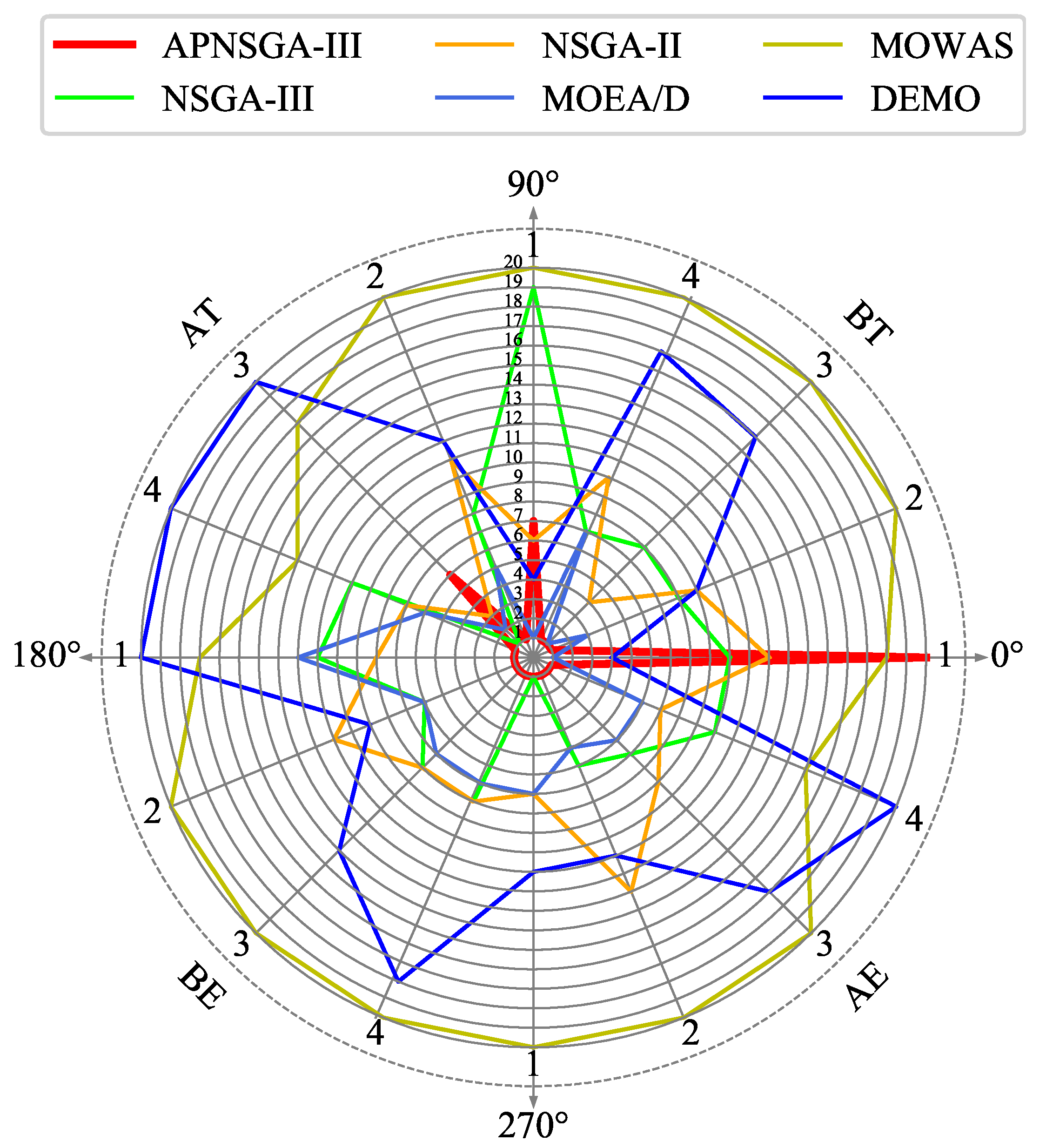
4.1. Result Show and Analysis

The final comparison results of I n s t a n c e 1 , 2 are placed in Table 11, while the final comparison results of I n s t a n c e 3 , 4 are placed in Table 12. BT and BE denotes the minimum completion time and minimum processing energy consumption, respectively. AT and AE implies the average completion time and average processing energy consumption, respectively. For I n s t a n c e 1 , APNSGA-III obtains the optima on BE and AE, while APNSGA-III can get the optima on BT, BE, and AE for I n s t a n c e 3 . Better, APNSGA-III can obtain the optima on BT, AT, BE, and AE for I n s t a n c e 2 and I n s t a n c e 4 . The performance of APNSGA-III far exceeds the other five comparison algorithms. In order to show the comparison of the algorithms in each goal more clearly, we rank the data in Table 11 and Table 12 on a level of 1–20 from big to small and visually show them in Figure 4. The area from 0 π / 2 , π / 2 π , π 3 π / 2 , 3 π / 2 2 π represents the ranking situation in B T , A T , B E , and A E , respectively. The Arabic numerals 1–4 around the circle represent I n s t a n c e 1–4. We can see that the area enclosed by the thick red line representing APNSGA-III is the smallest. Comprehensively, we can conclude that the DCS is valid and APNSGA-III is fit to solve the actual question we designed.

4.2. Two Independent Sample T-Tests

Due to the small sample size included in our experiment, we need to use two independent sample t-tests to test whether there is an accidental similarity between APNSGA-III and other comparison algorithms. We set 0.05 as the level of significance. The hypothesis is accepted when p > 0.05 , thus the test results indicate no significant difference between the two compared algorithms. The hypothesis is rejected when p < = 0.05 , thus the test results indicate significant differences between the APNSGA-III and contrasted algorithms. We will use the results of ten rounds of experiments that have been used to generate the average results in Table 11 and Table 12 as the test sample. The test results are shown in Table 13 and Table 14. We denote the value of p more than 0.05 as “+” and denote the value of p less than 0.05 as . ‘Same’ denotes the total number of APNSGA-III has no significant difference with other algorithms, while ’Better’ represents the total number of APNSGA-III that has significant differences with other algorithms.
From Table 13 and Table 14, we find that APNSGA-III and other algorithms are significantly different in almost all instances. Among the compared algorithms, NSGA-III is the closest to APNSGA-III, but there are still many differences between both. In general, we can conclude that APNSGA-III is significantly more excellent than the other algorithms.

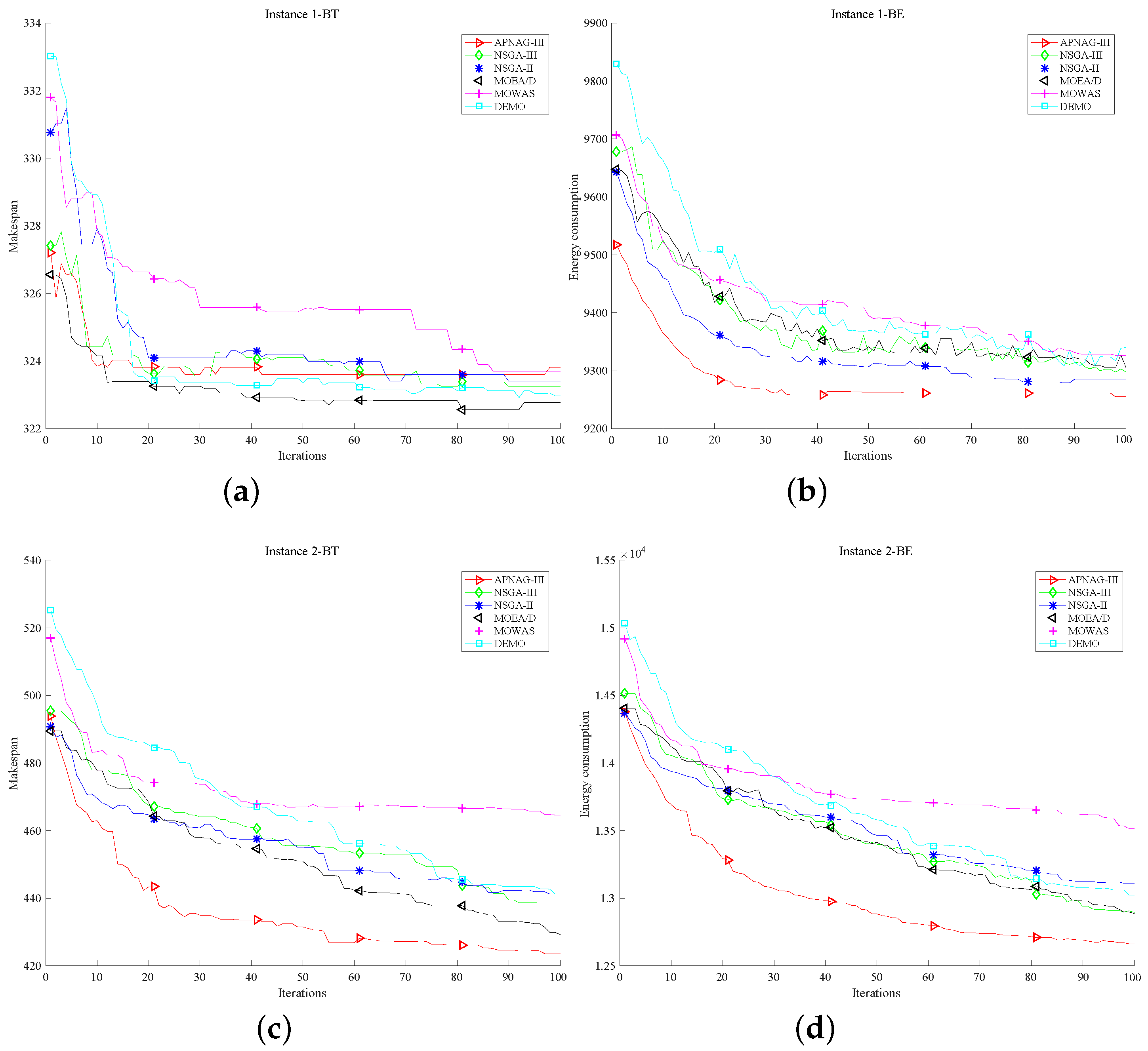
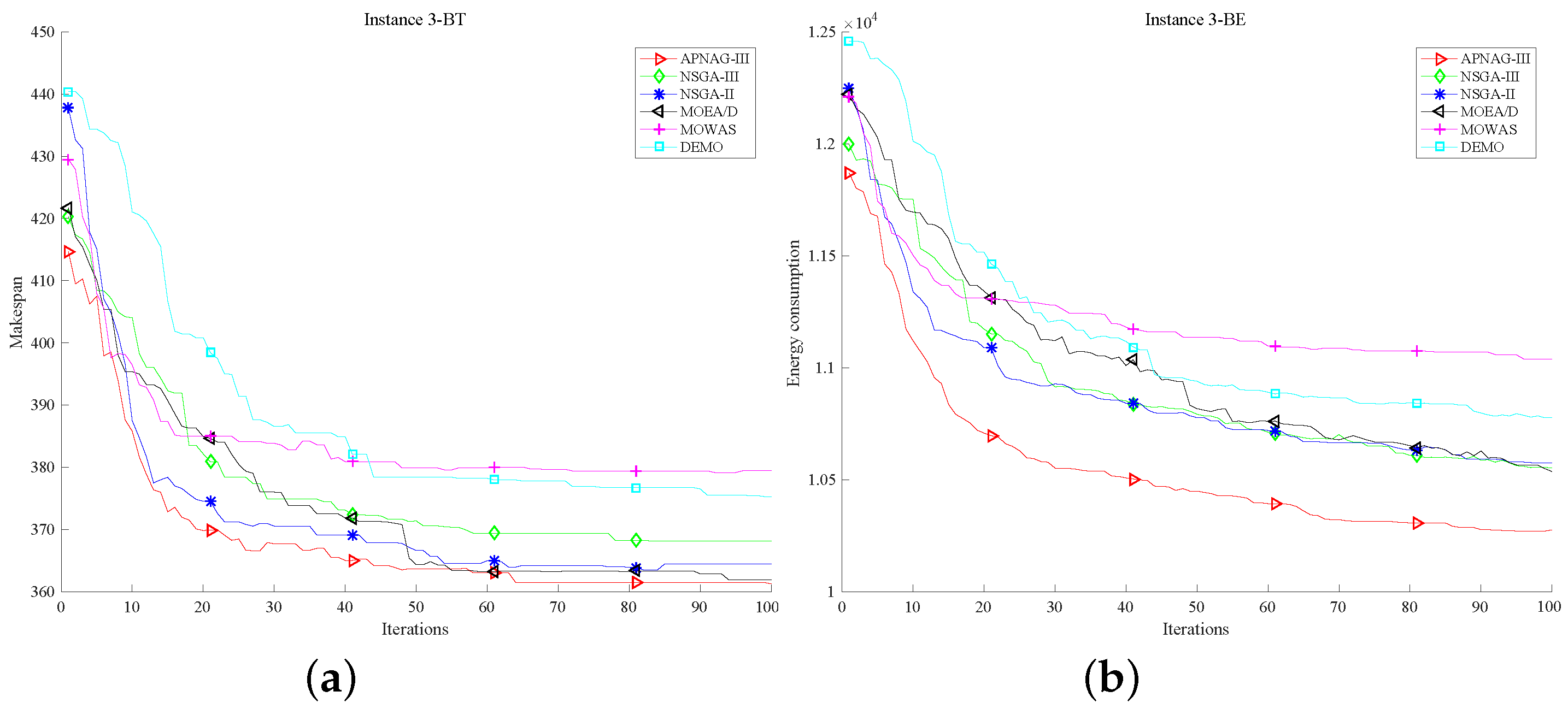
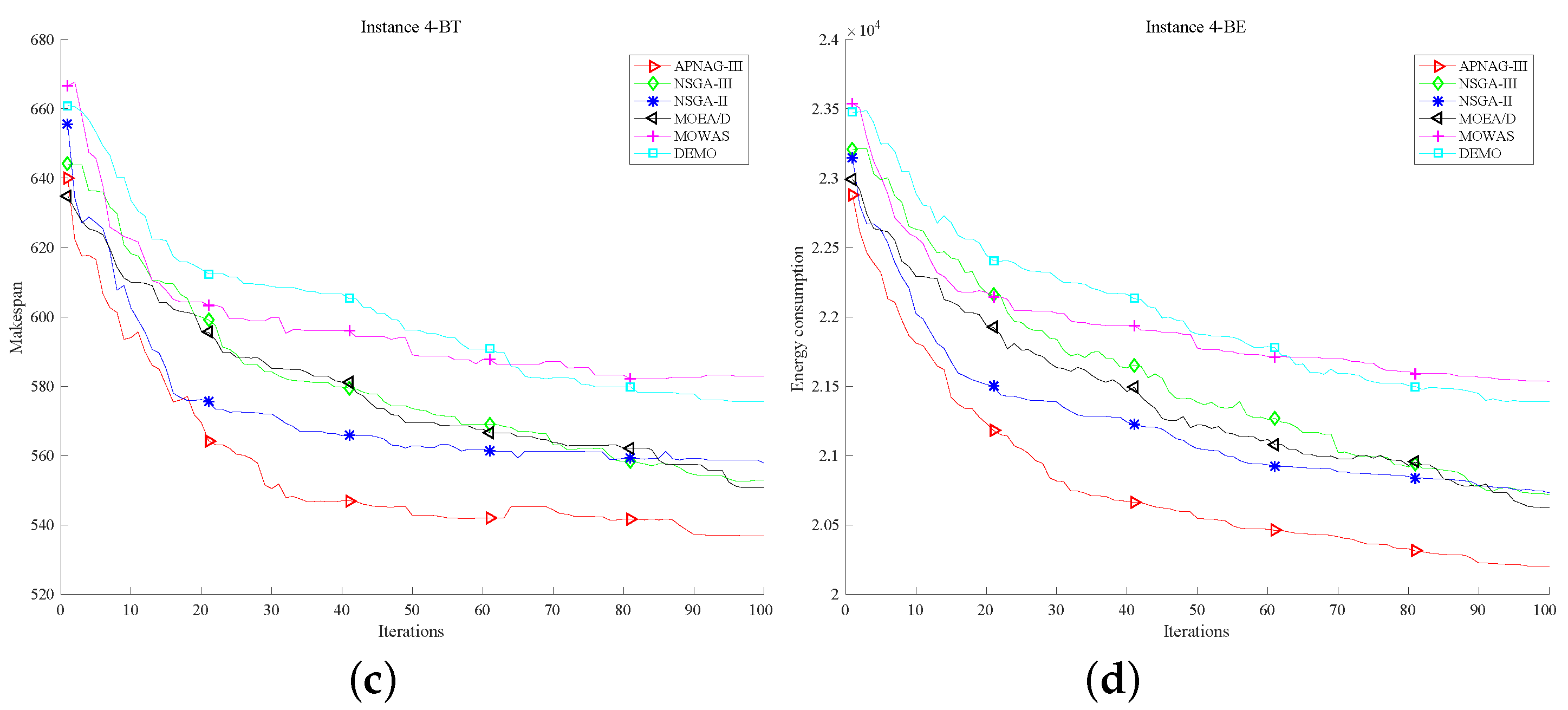
4.3. Convergence Analysis

This subsection shows the convergence of BT, ET for I n s t a n c e 1–4 in Figure 5 and Figure 6, respectively, and discusses the algorithm’s performance in the generation. The red line representing APNSGA-III always converges to the lowest position in the end except for part (a) of Figure 5. Moreover, the red line is almost below the other color lines in parts (b), (c), and (d) of Figure 5 and Figure 6. It means the performance of each stage of the entire optimization process of APNSGA-III is better than other comparison algorithms. It once again confirms the improvement of DCS and the excellent applicability of APNSGA-III.

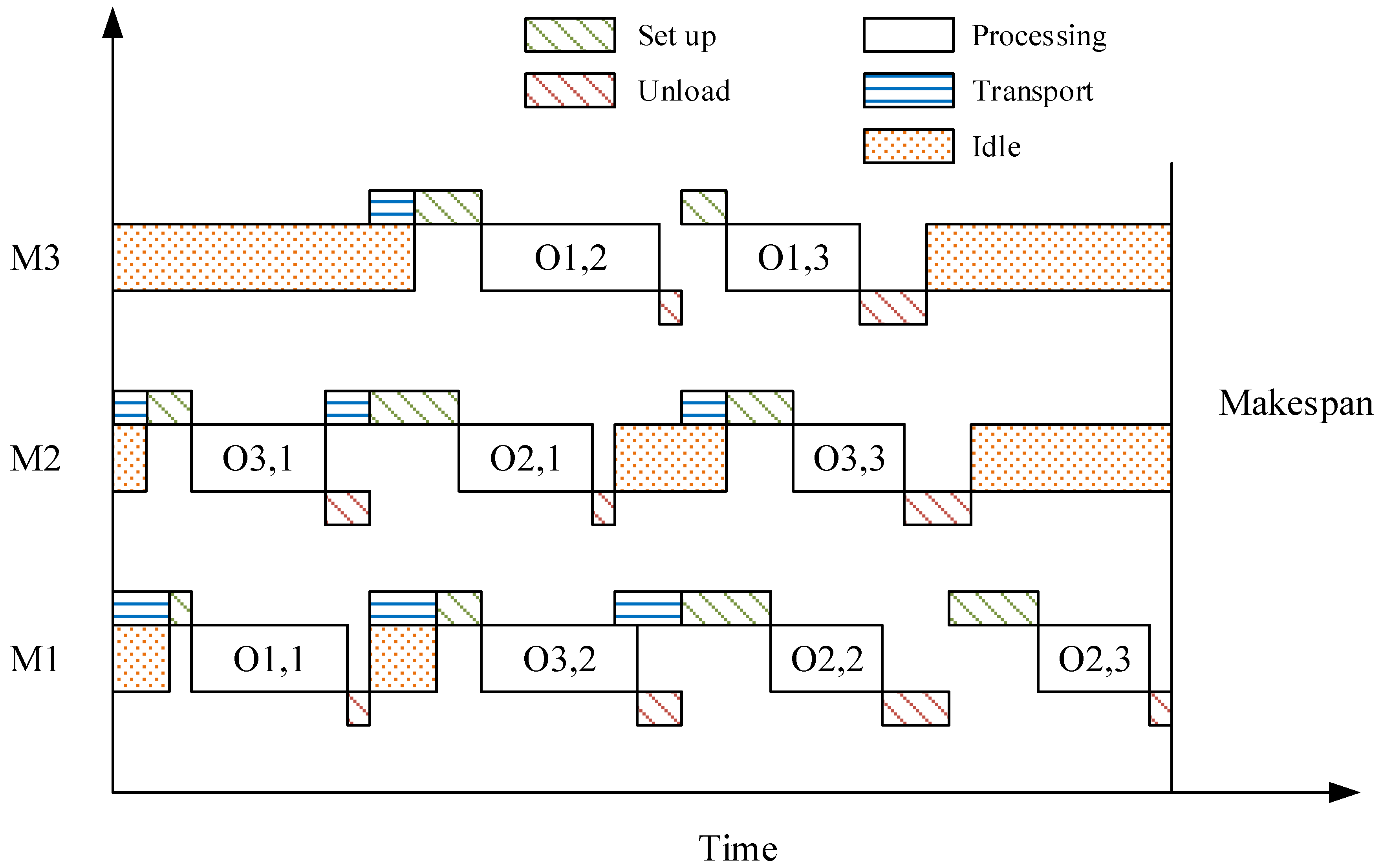
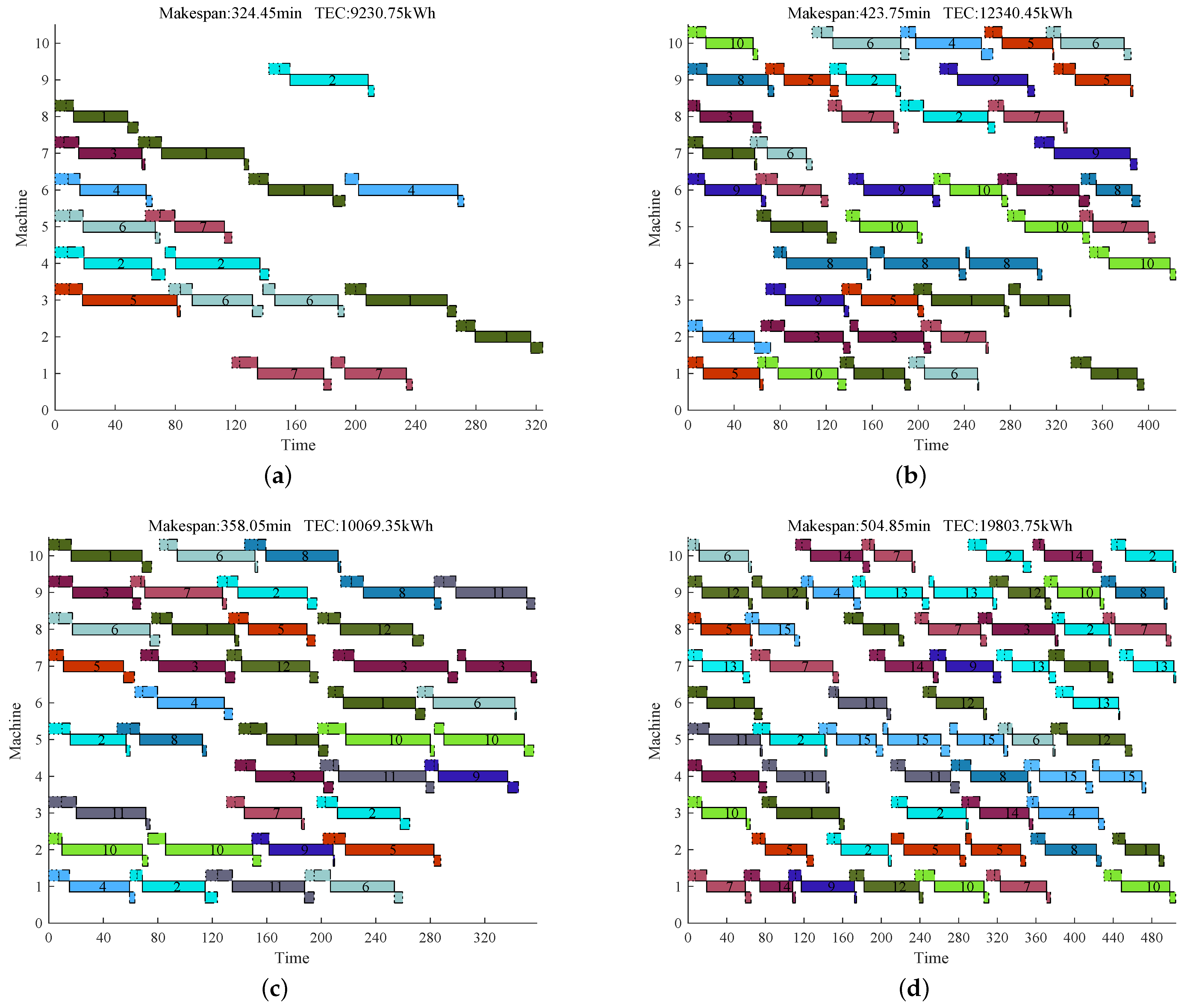
4.4. Gantt Chart Display and Analysis

The Gantt chart of I n s t a n c e 1–4 with the smallest energy consumption is shown in Figure 7. For I n s t a n c e 1 , the M a k e s p a n and T E C is 324.45 min and 9230.75 kWh, respectively. For I n s t a n c e 2 , the M a k e s p a n and T E C is 423.75 min and 12,340.45 kWh, respectively. For I n s t a n c e 3 , the M a k e s p a n and T E C is 358.05 min and 10,069.35 kWh, respectively. For I n s t a n c e 4 , the M a k e s p a n and T E C is 504.85 min and 19,803.75 kWh, respectively. There are few gaps for I n s t a n c e 2–4. It means that our method is effective, and the final scheduling plan has considerable advantages. In addition to the processing stage, the other three stages, set up, unload, and idle, also occupy a large proportion in the Gantt chart, especially in part (a); a large number of gaps means that the machine is at no load many times. This is also a large part of the energy consumption. If this part of energy consumption is not counted as the total energy consumption, it is impossible to make an accurate energy consumption analysis based on the existing scheduling situation, and thus it is impossible to achieve effective energy conservation.

5. Conclusions

Considering the previous research which mostly concentrates more on efficiency and ignores energy consumption, this paper designs the FJSP model with consideration of energy consumption. Meanwhile, the work includes non-negligible energy consumption, including the transport, set up, unload, and idle stage. The weight property of the job is also considered in our model. Besides, a dual control strategy for multi-objective optimization is designed to enhance the performance of NSGA-III when faced with multi-objective FJSP. Four FJSP instances are formulated to examine the metrics of our algorithm. The results obtained by APNSGA-III are compared with another five classic multi-objective optimization algorithms. All of the results reply that Diagonal Orthant Latent Dirichlet Allocation (DOLDA) owns a competitive superiority in solving the global optimization of these FJSP instances. In conclusion, the proposed algorithm shows a performance improvement compared with other multi-objective optimization algorithms, but further studies on the model accuracy and computation time are required through investigating more energy-efficient scheduling problem. On the other hand, unexpected events, such as machine failure, rush orders, and job cancellation, which may occur in the practical applications of a manufacturing system, should be considered in our FJSP. Reducing the energy consumption in a dynamic scheduling problem should also be studied in the future.

Author Contributions

Conceptualization, Z.Y.; Data curation, M.W. and B.Z.; Funding acquisition, D.Y.; Investigation, M.W. and T.L.; Methodology, Z.Y.; Project administration, D.Y.; Resources, B.Z., L.L., Z.W. and K.H.; Software, M.W.; Writing—original draft, M.W.; Writing—review & editing, Z.Y. All authors have read and agreed to the published version of the manuscript.

Funding

This research was funded by [National Key R&D Program of China] grant number [2018YFB1700500] and [National Science Foundation of China under grants] grant number [52077213 and 62003332]. The APC was funded by [National Key R&D Program of China] grant number [2018YFB1700500] and [National Science Foundation of China under grants] grant number [52077213 and 62003332].

Institutional Review Board Statement

Not applicable.

Informed Consent Statement

Not applicable.

Data Availability Statement

Not applicable.

Acknowledgments

This work was supported by the National Key R&D Program of China (2018YFB1700500) and the National Science Foundation of China under grants (52077213 and 62003332).

Conflicts of Interest

The authors declare no conflict of interest.

References

  1. Dai, M.; Tang, D.; Giret, A.; Salido, M.A. Multi-objective optimization for energy-efficient flexible job shop scheduling problem with transportation constraints. Robot. Comput.-Integr. Manuf. 2019, 59, 143–157. [Google Scholar] [CrossRef]
  2. Caldeira, R.H.; Gnanavelbabu, A.; Vaidyanathan, T. An effective backtracking search algorithm for multi-objective flexible job shop scheduling considering new job arrivals and energy consumption. Comput. Ind. Eng. 2020, 149, 106863. [Google Scholar] [CrossRef]
  3. Gong, X.; De Pessemier, T.; Martens, L.; Joseph, W. Energy-and labor-aware flexible job shop scheduling under dynamic electricity pricing: A many-objective optimization investigation. J. Clean. Prod. 2019, 209, 1078–1094. [Google Scholar] [CrossRef] [Green Version]
  4. Zhang, Z.; Wu, L.; Peng, T.; Jia, S. An improved scheduling approach for minimizing total energy consumption and makespan in a flexible job shop environment. Sustainability 2019, 11, 179. [Google Scholar] [CrossRef] [Green Version]
  5. Salido, M.A.; Escamilla, J.; Giret, A.; Barber, F. A genetic algorithm for energy-efficiency in job-shop scheduling. Int. J. Adv. Manuf. Technol. 2016, 85, 1303–1314. [Google Scholar] [CrossRef]
  6. Bányai, T. Optimization of Material Supply in Smart Manufacturing Environment: A Metaheuristic Approach for Matrix Production. Machines 2021, 9, 220. [Google Scholar] [CrossRef]
  7. Li, M.; Lei, D. An imperialist competitive algorithm with feedback for energy-efficient flexible job shop scheduling with transportation and sequence-dependent setup times. Eng. Appl. Artif. Intell. 2021, 103, 104307. [Google Scholar] [CrossRef]
  8. Gordillo, A.; Giret, A. Performance Evaluation of Bidding-Based Multi-Agent Scheduling Algorithms for Manufacturing Systems. Machines 2014, 2, 233–254. [Google Scholar] [CrossRef] [Green Version]
  9. Liu, Y.; Dong, H.; Lohse, N.; Petrovic, S.; Gindy, N. An investigation into minimising total energy consumption and total weighted tardiness in job shops. J. Clean. Prod. 2014, 65, 87–96. [Google Scholar] [CrossRef]
  10. Feng, Y.; Liu, M.; Zhang, Y.; Wang, J. A Dynamic Opposite Learning Assisted Grasshopper Optimization Algorithm for the Flexible JobScheduling Problem. Complexity 2020, 2020, 8870783. [Google Scholar] [CrossRef]
  11. Yin, L.; Li, X.; Gao, L.; Lu, C.; Zhang, Z. Energy-efficient job shop scheduling problem with variable spindle speed using a novel multi-objective algorithm. Adv. Mech. Eng. 2017, 9, 1687814017695959. [Google Scholar] [CrossRef] [Green Version]
  12. Gabriel, F.; Baars, S.; Römer, M.; Dröder, K. Grasp Point Optimization and Leakage-Compliant Dimensioning of Energy-Efficient Vacuum-Based Gripping Systems. Machines 2021, 9, 149. [Google Scholar] [CrossRef]
  13. Zhu, Z.; Lu, L.; Zhang, W.; Liu, W. EIA’s International Energy Outlook Analyzes Electricity Markets in India, Africa, and Asia. 2020. Available online: https://www.eia.gov/outlooks/ieo/ (accessed on 10 November 2021).
  14. Pereira, A.C.; Romero, F. A review of the meanings and the implications of the Industry 4.0 concept. Procedia Manuf. 2017, 13, 1206–1214. [Google Scholar] [CrossRef]
  15. Zhang, S.; Du, H.; Borucki, S.; Jin, S.; Hou, T.; Li, Z. Dual Resource Constrained Flexible Job Shop Scheduling Based on Improved Quantum Genetic Algorithm. Machines 2021, 9, 108. [Google Scholar] [CrossRef]
  16. Gadaleta, M.; Pellicciari, M.; Berselli, G. Optimization of the energy consumption of industrial robots for automatic code generation. Robot. Comput.-Integr. Manuf. 2019, 57, 452–464. [Google Scholar] [CrossRef]
  17. Del Pero, F.; Berzi, L.; Antonacci, A.; Delogu, M. Automotive Lightweight Design: Simulation Modeling of Mass-Related Consumption for Electric Vehicles. Machines 2020, 8, 51. [Google Scholar] [CrossRef]
  18. Hong, E.; Yeneneh, A.M.; Sen, T.K.; Ang, H.M.; Kayaalp, A. A comprehensive review on rheological studies of sludge from various sections of municipal wastewater treatment plants for enhancement of process performance. Adv. Colloid Interface Sci. 2018, 257, 19–30. [Google Scholar] [CrossRef]
  19. Wu, M.; Yang, D.; Yang, Z.; Guo, Y. Sparrow Search Algorithm for Solving Flexible Jobshop Scheduling Problem. In Proceedings of the International Conference on Swarm Intelligence, Qingdao, China, 17–21 July 2021; pp. 140–154. [Google Scholar]
  20. Gholami, O.; Sotskov, Y.N. A fast heuristic algorithm for solving parallel-machine job-shop scheduling problems. Int. J. Adv. Manuf. Technol. 2014, 70, 531–546. [Google Scholar] [CrossRef]
  21. Chaudhry, I.A.; Khan, A.A. A research survey: Review of flexible job shop scheduling techniques. Int. Trans. Oper. Res. 2016, 23, 551–591. [Google Scholar] [CrossRef]
  22. Gu, X.; Huang, M.; Liang, X. An improved genetic algorithm with adaptive variable neighborhood search for FJSP. Algorithms 2019, 12, 243. [Google Scholar] [CrossRef] [Green Version]
  23. Meng, L.; Zhang, C.; Shao, X.; Ren, Y. MILP models for energy-aware flexible job shop scheduling problem. J. Clean. Prod. 2019, 210, 710–723. [Google Scholar] [CrossRef]
  24. Zeng, Q.; Wang, M.; Shen, L.; Song, H. Sequential scheduling method for FJSP with multi-objective under mixed work calendars. Processes 2019, 7, 888. [Google Scholar] [CrossRef] [Green Version]
  25. Manne, A.S. On the job-shop scheduling problem. Oper. Res. 1960, 8, 219–223. [Google Scholar] [CrossRef] [Green Version]
  26. Yang, D.; Wu, M.; Yang, Z.; Guo, Y.; Feng, W. Dragonfly algorithm for Solving Flexible Jobshop Scheduling Problem. In Proceedings of the 2020 35th Youth Academic Annual Conference of Chinese Association of Automation (YAC), Zhanjiang, China, 16–18 October 2020; pp. 867–872. [Google Scholar]
  27. Zhang, H.; Xu, G.; Pan, R.; Ge, H. A novel heuristic method for the energy-efficient flexible job-shop scheduling problem with sequence-dependent set-up and transportation time. In Engineering Optimization; Taylor & Francis: Abingdon, UK, 2021; pp. 1–22. [Google Scholar]
  28. Park, J.S.; Ng, H.Y.; Chua, T.J.; Ng, Y.T.; Kim, J.W. Unified genetic algorithm approach for solving flexible job-shop scheduling problem. Appl. Sci. 2021, 11, 6454. [Google Scholar] [CrossRef]
  29. Lei, D.; Li, M.; Wang, L. A two-phase meta-heuristic for multiobjective flexible job shop scheduling problem with total energy consumption threshold. IEEE Trans. Cybern. 2018, 49, 1097–1109. [Google Scholar] [CrossRef]
  30. Luan, F.; Cai, Z.; Wu, S.; Liu, S.Q.; He, Y. Optimizing the low-carbon flexible job shop scheduling problem with discrete whale optimization algorithm. Mathematics 2019, 7, 688. [Google Scholar] [CrossRef] [Green Version]
  31. Mouzon, G.; Yildirim, M.B.; Twomey, J. Operational methods for minimization of energy consumption of manufacturing equipment. Int. J. Prod. Res. 2007, 45, 4247–4271. [Google Scholar] [CrossRef] [Green Version]
  32. Lei, D.; Zheng, Y.; Guo, X. A shuffled frog-leaping algorithm for flexible job shop scheduling with the consideration of energy consumption. Int. J. Prod. Res. 2017, 55, 3126–3140. [Google Scholar] [CrossRef]
  33. Wu, X.; Shen, X.; Li, C. The flexible job-shop scheduling problem considering deterioration effect and energy consumption simultaneously. Comput. Ind. Eng. 2019, 135, 1004–1024. [Google Scholar] [CrossRef]
  34. Wu, X.; Sun, Y. A green scheduling algorithm for flexible job shop with energy-saving measures. J. Clean. Prod. 2018, 172, 3249–3264. [Google Scholar] [CrossRef]
  35. Wang, F.; Liao, F.; Li, Y.; Wang, H. A new prediction strategy for dynamic multi-objective optimization using Gaussian Mixture Model. Inf. Sci. 2021, 580, 331–351. [Google Scholar] [CrossRef]
  36. Zhang, G.; Shao, X.; Li, P.; Gao, L. An effective hybrid particle swarm optimization algorithm for multi-objective flexible job-shop scheduling problem. Comput. Ind. Eng. 2009, 56, 1309–1318. [Google Scholar] [CrossRef]
  37. Gao, K.Z.; Suganthan, P.N.; Pan, Q.K.; Chua, T.J.; Cai, T.X.; Chong, C.S. Discrete harmony search algorithm for flexible job shop scheduling problem with multiple objectives. J. Intell. Manuf. 2016, 27, 363–374. [Google Scholar] [CrossRef]
  38. Li, J.q.; Pan, Q.k.; Liang, Y.C. An effective hybrid tabu search algorithm for multi-objective flexible job-shop scheduling problems. Comput. Ind. Eng. 2010, 59, 647–662. [Google Scholar] [CrossRef]
  39. Lu, C.; Li, X.; Gao, L.; Liao, W.; Yi, J. An effective multi-objective discrete virus optimization algorithm for flexible job-shop scheduling problem with controllable processing times. Comput. Ind. Eng. 2017, 104, 156–174. [Google Scholar] [CrossRef]
  40. Álvarez-Gil, N.; Rosillo, R.; de la Fuente, D.; Pino, R. A discrete firefly algorithm for solving the flexible job-shop scheduling problem in a make-to-order manufacturing system. Cent. Eur. J. Oper. Res. 2021, 29, 1353–1374. [Google Scholar] [CrossRef]
  41. Chen, R.; Yang, B.; Li, S.; Wang, S. A self-learning genetic algorithm based on reinforcement learning for flexible job-shop scheduling problem. Comput. Ind. Eng. 2020, 149, 106778. [Google Scholar] [CrossRef]
  42. Li, J.q.; Deng, J.w.; Li, C.y.; Han, Y.y.; Tian, J.; Zhang, B.; Wang, C.g. An improved Jaya algorithm for solving the flexible job shop scheduling problem with transportation and setup times. Knowl.-Based Syst. 2020, 200, 106032. [Google Scholar] [CrossRef]
  43. Caldeira, R.H.; Gnanavelbabu, A. A Pareto based discrete Jaya algorithm for multi-objective flexible job shop scheduling problem. Expert Syst. Appl. 2021, 170, 114567. [Google Scholar] [CrossRef]
  44. Wang, Z.Y.; Lu, C. An integrated job shop scheduling and assembly sequence planning approach for discrete manufacturing. J. Manuf. Syst. 2021, 61, 27–44. [Google Scholar] [CrossRef]
  45. Wang, F.; Zhang, H.; Zhou, A. A particle swarm optimization algorithm for mixed-variable optimization problems. Swarm Evol. Comput. 2021, 60, 100808. [Google Scholar] [CrossRef]
  46. Feng, W.A.; Yl, A.; Fl, A.; Hy, B. An ensemble learning based prediction strategy for dynamic multi-objective optimization-ScienceDirect. Appl. Soft Comput. 2020, 96, 106592. [Google Scholar]
  47. Gong, G.; Deng, Q.; Gong, X.; Huang, D. A non-dominated ensemble fitness ranking algorithm for multi-objective flexible job-shop scheduling problem considering worker flexibility and green factors. Knowl.-Based Syst. 2021, 231, 107430. [Google Scholar] [CrossRef]
  48. Deb, K.; Jain, H. An evolutionary many-objective optimization algorithm using reference-point-based nondominated sorting approach, part I: Solving problems with box constraints. IEEE Trans. Evol. Comput. 2013, 18, 577–601. [Google Scholar] [CrossRef]
  49. Zhang, G.; Gao, L.; Shi, Y. An effective genetic algorithm for the flexible job-shop scheduling problem. Expert Syst. Appl. 2011, 38, 3563–3573. [Google Scholar] [CrossRef]
  50. Ishikawa, S.; Kubota, R.; Horio, K. Effective hierarchical optimization by a hierarchical multi-space competitive genetic algorithm for the flexible job-shop scheduling problem. Expert Syst. Appl. 2015, 42, 9434–9440. [Google Scholar] [CrossRef]
  51. Zhang, X.; Zhan, Z.H.; Zhang, J. Adaptive Population Differential Evolution with Dual Control Strategy for Large-Scale Global optimization Problems. In Proceedings of the 2020 IEEE Congress on Evolutionary Computation (CEC), Glasgow, UK, 19–24 July 2020; pp. 1–7. [Google Scholar]
  52. Deb, K.; Pratap, A.; Agarwal, S.; Meyarivan, T. A fast and elitist multiobjective genetic algorithm: NSGA-II. IEEE Trans. Evol. Comput. 2002, 6, 182–197. [Google Scholar] [CrossRef] [Green Version]
  53. Zhang, Q.; Li, H. MOEA/D: A multiobjective evolutionary algorithm based on decomposition. IEEE Trans. Evol. Comput. 2007, 11, 712–731. [Google Scholar] [CrossRef]
  54. Wang, G.; Gao, L.; Li, X.; Li, P.; Tasgetiren, M.F. Energy-efficient distributed permutation flow shop scheduling problem using a multi-objective whale swarm algorithm. Swarm Evol. Comput. 2020, 57, 100716. [Google Scholar] [CrossRef]
  55. Han, Y.; Li, J.; Sang, H.; Liu, Y.; Pan, Q. Discrete evolutionary multi-objective optimization for energy-efficient blocking flow shop scheduling with setup time. Appl. Soft Comput. 2020, 93, 106343. [Google Scholar] [CrossRef]
Figure 1. Main structure of our FJSP model.
Machines 09 00344 g001
Figure 2. The Gantt chart of the instance mentioned before.
Machines 09 00344 g002
Figure 3. The flowchart of APNSGA-III.
Machines 09 00344 g003
Figure 4. Ranking of six algorithm.
Machines 09 00344 g004
Figure 5. The convergence curve of BT and BE for I n s t a n c e 1 and I n s t a n c e 2 . (a) BT of I n s t a n c e 1 ; (b) BE of I n s t a n c e 1 ; (c) BT of I n s t a n c e 2 ; (d) BE of I n s t a n c e 2 .
Machines 09 00344 g005
Figure 6. The convergence curve of BT and BE for I n s t a n c e 3 and I n s t a n c e 4 . (a) BT of I n s t a n c e 3 ; (b) BE of I n s t a n c e 3 ; (c) BT of I n s t a n c e 4 ; (d) BE of I n s t a n c e 4 .
Machines 09 00344 g006aMachines 09 00344 g006b
Figure 7. The Gantt chart of I n s t a n c e 1–4 with the smallest energy consumption. (a) The Gantt chart of I n s t a n c e 1; (b) the Gantt chart of I n s t a n c e 2; (c) the Gantt chart of I n s t a n c e 3; (d) the Gantt chart of I n s t a n c e 4.
Machines 09 00344 g007
Table 1. The processing information of the instance mentioned before (unit: min/kWh).
JobOperationMachine(Processing Time/Energy, Set Up Time/Energy, Unload Time/Energy)
O 11 M 2 , M 3 (40/46,9/21,2/11) (46/65,7/21,8/16)
J 1 O 12 M 3 , M 1 (53/46,7/9,7/6)(55/55,13/14,5/7)
O 13 M 2 , M 1 (55/64,8/18,6/4)(55/59,9/10,2/11)
O 21 M 1 , M 2 (56/79,7/11,2/11) (53/77,10/48,8/7)
J 2 O 22 M 2 , M 3 (62/76,4/17,5/7)(54/77,4/26,5/16)
O 23 M 2 , M 3 (62/59,6/21,8/2)(52/59,12/17,7/10)
O 31 M 3 , M 2 (50/50,10/21,5/4) (32/52,7/21,7/4)
J 3 O 32 M 3 , M 1 (35/71,7/20,6/13)(41/83,8/23,9/15)
O 33 M 3 , M 1 (49/89,5/18,6/16)(63/76,12/16,9/14)
Table 2. The transportation times of AGV between machines (unit: s).
Machine NumberMachine 1 ( M 1 )Machine 2 ( M 2 )Machine 3 ( M 3 )
Machine 1 ( M 1 )01518
Machine 2 ( M 2 )15012
Machine 3 ( M 3 )18120
Table 3. The FJSP instances generation rules.
ObjectiveStageaprocmot
TimeProcess40–60 [ 10 , 9 , 8 , 7 , 6 , 5 , 4 , 3 , 2 , 1 , 0 , 1 , 2 , 3 , 4 , 5 , 6 , 7 , 8 , 9 , 10 ]
Set up5–10 [ 2 , 1 , 0 , 1 , 2 , 3 ]
Unload3–6 [ 3 , 2 , 1 , 0 , 1 , 2 , 3 ]
EnergyProcess50-80 [ 10 , 9 , 8 , 7 , 6 , 5 , 4 , 3 , 2 , 1 , 0 , 1 , 2 , 3 , 4 , 5 , 6 , 7 , 8 , 9 , 10 ]
Set up10–20 [ 6 , 5 , 4 , 3 , 2 , 1 , 0 , 1 , 2 , 3 , 4 , 5 , 6 ]
Unload5–10 [ 4 , 3 , 2 , 1 , 0 , 1 , 2 , 3 , 4 , 5 , 6 ]
aproc: time or energy consumption per operation; mot: offset time or energy consumption boundaries on per machine.
Table 4. The general information of four instances.
Instancenjobnmacnopmeq
Instance 1610[1,2,3,4,5][1,2,3,4,5]
Instance 21010[2,3,4,5,6][1,2,3,4,5]
Instance 31210[2,3,4,5][1,2,3,4,5]
Instance 41510[2,3,4,5,6][1,2,3,4,5]
njob: number of jobs; nmac: number of machines; nop: minimum and maximum number of operation per job; meq: maximum number of available machine per operation.
Table 5. The weight information of the job in each instance (unit: kg).
Instance NameJobs
J 1 J 2 J 3 J 4 J 5 J 6 J 7 J 8 J 9 J 10 J 11 J 12 J 13 J 14 J 15
Instance 185962103--------
Instance 211042772393-----
Instance 3531321173988---
Instance 410736710387884639
Table 6. The transport time between machines (unit: s).
MachineOrigin M 1 M 2 M 3 M 4 M 5 M 6 M 7 M 8 M 9 M 10
Origing0144134185165194172116146149150
M 1 1440152170193100112173165142133
M 2 1341520131138152169120170162143
M 3 1851701310160151140132171122140
M 4 1651931381600140140165170140198
M 5 1941001521511400103102170180192
M 6 1721121691401401030142140148150
M 7 1161731201321651021420150162160
M 8 1461651701711701701401500141120
M 9 1491421621221401801481621410153
M 10 1501331431401981921501601201530
Table 7. The job shop information of I n s t a n c e 1 .
JobOperationMachineSet Up Time
(min)
Set Up Energy
Consumption (kWh)
Processing Time
(min)
Processing Energy
Consumption (kWh)
Unload Time
(min)
Unlaod Energy
Consumption (kWh)
J 1 O 11 [6,1,7,8,4][10,4,4,5,10][8,13,15,5,6][43,48,47,36,53][62,70,71,58,71][5,3,7,7,3][14,11,13,7,5]
O 12 [4,7,9,1][11,8,8,11][19,10,18,17][69,55,58,51][64,58,54,64][7,3,5,4][5,9,5,12]
O 13 [6,8,1][6,9,9][12,19,21][43,52,46][48,60,58][8,3,8][8,16,16]
O 14 [3][7][12][54][74][6][9]
O 15 [6,2,1,7][4,6,3,5][11,19,23,21][55,37,49,48][66,55,64,67][6,8,3,5][8,8,4,9]
J 2 O 21 [4][11][10][45][54][9][6]
O 22 [4,1,3][7,12,12][23,15,24][56,44,56][80,89,71][6,6,8][11,7,4]
O 23 [9,7,3][7,9,5][13,18,16][52,57,55][52,52,59][4,4,4][11,13,6]
J 3 O 31 [7,4,10][17,15,17][15,18,17,12,16][42,55,40][77,79,70][2,2,5][9,12,10]
J 4 O 41 [6,4][8,7][16,24][44,58][70,82][4,5][2,12]
O 42 [5,6,4,9,1][8,9,4,5,9][10,6,13,7,18][52,66,63,56,51][54,64,51,63,49][5,4,8,2,6][7,11,13,13,11]
J 5 O 51 [4,6,3,8][5,3,9,3][18,22,19,22][59,61,63,55][64,48,53,62][5,2,2,7][7,10,4,6]
J 6 O 61 [5][9][15][48][65][3][14]
O 62 [3,6][8,10][10,19][40,42][65,56][7,7][14,10]
O 63 [1,10,7,3,8][5,10,11,8,6][17,16,7,10,7][43,45,52,42,46][72,70,80,77,71][8,7,8,4,5][14,9,12,10,13]
J 7 O 71 [9,5][8,10][17,15][34,33][53,49][5,5][12,11]
O 72 [1,5][12,6][11,18][44,33][62,66][5,3][13,12]
O 73 [9,1][10,9][21,17][54,41][74,63][7,4][9,10]
Table 8. The job shop information of I n s t a n c e 2 .
JobOperationMachineSet Up Time
(min)
Set Up Energy
Consumption (kWh)
Processing Time
(min)
Processing Energy
Consumption (kWh)
Unload Time
(min)
Unlaod Energy
Consumption (kWh)
J 1 O 11 [7,2,6][7,6,11][15,11,21][45,54,55][59,76,58][2,8,7][10,6,12]
O 12 [7,5][6,7][12,11][61,49][67,59][7,8][11,5]
O 13 [1][7][8][44][51][5][12]
O 14 [5,1,3,10][5,9,7,8][9,18,8,10][53,52,63,56][79,69,83,87][4,4,4,3][2,11,12,9]
O 15 [3,2,6][10,13,7][19,22,21][43,42,44][54,49,49][1,7,3][3,9,8]
O 16 [1,7][9,11][15,11][40,48][47,48][6,9][5,2]
J 1 O 21 [2,3,9,10,7][8,11,7,10,8][19,21,22,23,17][53,43,43,54,47][59,52,62,68,63][2,1,4,2,1][4,10,2,3,11]
O 22 [8,4][13,8][14,22][56,47][74,59][6,4][5,9]
J 3 O 31 [10,8][6,3][14,18][37,46][64,50][3,7][9,7]
O 32 [9,6,8,10,2][7,9,9,9,12][12,14,10,22,13][52,45,56,48,51][68,63,52,51,56][8,8,8,6,6][14,2,14,13,7]
O 33 [2][7][14][57][50][6][3]
O 34 [6][8][18][54][76][9][7]
J 4 O 41 [2][6][14][45][88][14][11]
O 42 [1,10,5,8,4][10,6,7,8,8][12,10,19,20,21][59,57,53,44,40][51,70,69,50,54][12,10,19,20,21][14,10,4,3,11]
J 5 O 51 [5,9,1,8][9,7,6,10][15,9,10,6][47,49,49,52][84,84,70,77][3,2,3,3][16,9,7,14]
O 52 [7,3,4,9,5][6,8,3,9,4][24,24,22,13,13][31,45,37,40,35][73,65,80,79,80][8,4,4,7,3][5,11,2,5,9]
O 53 [3,8][11,6][18,13][49,52][71,62][5,9][8,13]
O 54 [10,1][8,9][9,15][44,32][83,69][1,5][6,12]
O 55 [9,2][11,8][14,25][48,48][62,52][2,7][8,3]
J 6 O 61 [2,9,8,3,7][6,6,11,6,9][12,18,11,18,7][52,39,45,49,34][75,65,68,75,66][5,8,3,4,5][7,10,8,8,10]
O 62 [2,1,7,3,10][11,13,11,7,10][19,16,16,12,18][50,53,53,54,59][75,77,75,64,70][9,7,3,7,7][14,9,4,14,4]
O 63 [1,7][7,7][14,16][46,59][57,56][1,2][5,10]
O 64 [10,7,4][6,10,9][23,24,25][55,47,51][48,46,45][6,9,6][7,9,5]
J 7 O 71 [7,10,5,6,4][12,8,7,10,11][5,7,15,13,6][45,33,52,38,47][80,82,63,72,80][9,8,5,6,8][4,4,7,1,9]
O 72 [2,4,8,3,6][4,9,5,9,6][11,11,11,12,11][38,45,45,51,53][61,64,52,59,56][1,4,4,5,5][10,15,15,10,12]
O 73 [6,10,8,2,4][10,11,7,9,10][13,11,15,13,18][41,37,39,39,44][52,63,63,59,46][3,2,2,2,5][8,2,9,5,5]
O 74 [8,4,6][5,9,8][12,6,12][52,38,35][57,64,59][3,3,5][13,11,6]
O 75 [7,5][4,3][7,7][40,48][60,43][4,6][7,15]
J 8 O 81 [9,10][9,10][23,21][53,63][79,89][5,3][4,7]
O 82 [1,4,5,7,8][4,4,6,9,7][17,16,9,7,14][54,70,62,52,52][53,54,57,56,49][4,3,5,4,4][14,6,9,9,15]
O 83 [6,4,8,1,7][12,12,8,7,8][15,8,14,17,12][59,65,50,60,50][56,57,61,64,45][2,6,1,3,1][12,10,8,14,13]
O 84 [4,5,7,2,3][3,6,5,5,3][11,17,22,13,17][59,50,43,47,45][66,55,62,55,57][4,5,5,4,4][9,7,7,4,10]
O 85 [6][6][18][31][74][7][9]
J 9 O 91 [6][6][13][49][77][4][12]
O 92 [1,8,3][6,8,10][13,21,15][53,54,51][61,64,51][7,7,4][13,2,7]
O 93 [6][6][16][60][63][6][4]
O 94 [1,4,9,7][8,6,8,7][8,14,12,9][46,48,61,49][68,69,58,71][8,3,6,2][15,6,5,14]
O 95 [7,8,1,10][9,7,9,10][7,17,16,11][66,53,58,64][65,73,72,61][6,4,6,3][5,10,12,10]
J 10 O 101 [9,10][12,8][9,16][48,41][67,62][6,4][14,8]
O 102 [7,1][6,11][26,20][34,52][55,61][3,7][9,2]
O 103 [2,5,7,10,6][7,7,10,9,6][21,18,17,16,16][40,50,38,42,53][65,78,64,70,76][6,4,5,4,1][7,5,12,13,4]
O 104 [9,6,8][5,9,6][13,9,9][55,45,56][65,73,70][8,5,6][10,4,12]
O 105 [3,5][7,10][19,20][37,50][63,68][4,6][7,4]
O 106 [2,8,9,1,4][11,10,8,11,10][16,16,17,17,10][66,59,53,51,53][72,77,69,79,75][8,4,6,6,5][4,3,1,3,11]
Table 9. The job shop information of I n s t a n c e 3 .
JobOperationMachineSet Up Time
(min)
Set Up Energy
Consumption (kWh)
Processing Time
(min)
Processing Energy
Consumption (kWh)
Unload Time
(min)
Unlaod Energy
Consumption (kWh)
J 1 O 11 [10][9][9][52][69][7][15]
O 12 [8,3,4,9][9,6,4,8][12,15,13,13][46,48,46,44][71,68,78,69][3,6,3,4][4,9,12,9]
O 13 [6,1,5][10,12,12][17,11,8][42,56,38][58,52,57][3,6,7][11,11,11]
O 14 [6][6][8][53][64][7][13]
J 2 O 21 [6,5][6,6][15,9][45,41][78,68][8,3][4,3]
O 22 [1][4][18][46][50][9][10]
O 23 [8,4,9,6][7,8,8,9][15,16,19,18][56,42,51,52][52,68,59,56][3,5,7,8][10,7,6,10]
O 24 [3][9][12][46][71][7][3]
J 3 O 31 [7,10,8,9][10,9,8,10][15,12,20,21][51,56,58,44][68,56,50,61][4,7,3,6][8,13,3,13]
O 32 [2,1,7,9][6,8,5,9][11,11,21,16][60,68,49,58][68,79,75,85][8,5,7,7][9,11,12,8]
O 33 [4][7][12][50][68][7][3]
O 34 [7][7][16][69][59][7][11]
O 35 [5,3,6,1,7][9,6,10,11,6][8,13,15,9,11][43,42,52,42,48][87,82,75,89,76][5,5,9,8,4][6,4,5,8,2]
J 4 O 41 [10,7,8,5,1][6,4,4,7,8][20,12,19,20,19][41,49,37,50,44][54,65,50,45,54][5,6,6,4,4][6,8,4,0,6]
O 42 [5,8,4,6][6,10,10,11][15,19,12,10][39,49,40,49][69,76,65,71][5,5,4,6][11,6,12,11]
J 5 O 51 [10,9,2,7][10,9,9,5][16,12,12,9][41,36,42,44][60,55,61,58][7,3,8,8][12,6,4,5]
O 52 [8][7][14][43][83][6][11]
O 53 [8,2][10,8][14,13][58,65][88,86][3,5][5,1]
J 6 O 61 [8,9,2][10,11,11][18,19,18][57,53,61][59,60,71][7,1,7][14,12,4]
O 62 [3,5,10,1][7,9,7,6][8,13,15,16][42,51,57,41][50,60,64,48][2,4,2,2][8,1,8,7]
O 63 [5,1,6,9][13,12,9,9][15,23,13,18][36,47,37,48][52,52,65,72][5,6,9,5][6,6,14,11]
O 64 [3,5,2,6][9,10,5,6][16,17,17,17][42,42,40,60][83,72,86,74][4,1,1,1][10,3,8,3]
J 7 O 71 [4,9,10,7,1][6,3,3,8,8][10,17,11,11,19][51,57,61,59,60][78,79,79,66,76][5,3,3,3,4][13,9,13,11,15]
O 72 [3][7][22][42][70][2][2]
J 8 O 81 [5,2,6][7,5,5][14,24,22][46,45,38][80,76,65][3,4,4][8,9,9]
O 82 [10,2,5,4,3][6,5,3,5,6][10,16,13,17,15][53,49,40,48,49][62,59,56,51,54][2,2,5,2,6][2,13,13,12,5]
O 83 [8,9,2][8,9,9][14,7,11][57,52,40][79,62,63][3,5,8][10,2,10]
J 9 O 91 [1,9,10,3,2][7,9,9,10,6][20,16,17,15,11][50,50,40,43,47][80,82,85,69,80][2,5,6,5,1][6,9,12,16,9]
O 92 [4,7][3,9][18,23][51,51][46,43][8,8][9,11]
J 10 O 101 [2][3][13][59][80][4][3]
O 102 [6,4,2][10,10,13][19,21,17][50,55,64][62,60,55][5,3,6][10,13,3]
O 103 [2,5,4,1,10][11,13,7,8,13][13,7,12,16,11][49,62,49,48,55][67,78,80,69,71][6,3,3,6,8][4,2,11,9,12]
O 104 [4,9,3,5][9,6,3,7][17,25,21,13][51,60,60,59][77,74,86,79][6,7,5,7][9,5,4,5]
J 11 O 111 [1,3][11,11][22,19][64,51][58,66][4,3][10,1]
O 112 [1,10,5,4,2][11,12,10,8,9][8,15,17,14,18][53,41,53,46,39][74,78,69,74,72][7,7,7,6,6][3,2,10,8,8]
O 113 [4][4][18][64][69][6][10]
O 114 [10,9,3,2][12,9,11,13][16,10,18,15][46,52,51,50][72,71,64,69][6,6,4,4][8,13,8,11]
J 12 O 121 [4,10,2,7,5][10,7,10,5,8][15,18,12,13,19][53,55,59,50,62][56,65,62,60,74][5,5,3,6,9][4,8,1,1,6]
O 122 [6,8,5,7][11,9,10,9][20,21,20,18][54,53,56,66][64,55,56,61][5,8,3,5][14,13,13,14]
Table 10. The job shop information of I n s t a n c e 4 .
JobOperationMachineSet Up Time
(min)
Set Up Energy
Consumption (kWh)
Processing Time
(min)
Processing Energy
Consumption (kWh)
Unload Time
(min)
Unlaod Energy
Consumption (kWh)
J 1 O 11 [6][11][12][49][69][8][14]
O 12 [4,3][7,8][21,13][55,65][79,59][2,5][10,2]
O 13 [3,8,1][13,11,8][22,22,25][46,37,50][63,61,59][8,5,6][10,11,8]
O 14 [7,8,5,6][9,5,8,5][13,7,8,10][45,46,56,45][56,70,61,60][5,9,3,8][2,1,11,10]
O 15 [2,5][7,7][12,18][35,46][66,79][5,5][1,9]
J 2 O 21 [8,5,3][10,8,9][23,21,17][50,57,56][65,60,58][8,2,7][7,10,9]
O 22 [2,9,4][7,10,9][16,16,14][49,59,53][73,66,82][3,6,1][0,6,9]
O 23 [1,3][7,10][23,12][65,61][81,67][6,2][9,13]
O 24 [10,2,3][12,9,13][8,13,9][38,44,38][60,58,45][8,2,7][0,5,8]
O 25 [7,6,8,5][5,8,7,7][21,18,22,22][44,46,46,59][65,53,51,56][2,4,2,3][4,13,5,11]
O 26 [10][9][10][49][70][3][15]
J 3 O 31 [4][6][17][59][66][8][3]
O 32 [8][6][5][65][65][3][10]
J 4 O 41 [5,9,8][5,5,9][22,22,17][52,42,54][52,63,45][7,7,5][10,9,8]
O 42 [5,1,3][7,12,6][21,23,11][63,49,62][66,64,65][2,3,6][7,6,5]
J 5 O 51 [5,4,8,6][9,7,6,5][14,8,7,13][58,54,51,42][64,73,61,75][5,7,2,5][12,4,1,10]
O 52 [2,4][5,11][22,17][43,54][63,71][7,4][6,6]
O 53 [10,2][8,13][19,11][41,58][54,52][1,6][9,12]
O 54 [2,9][6,10][23,15][51,36][62,64][5,5][15,5]
J 6 O 61 [10,3][4,6][12,18][51,48][59,54][3,9][14,15]
O 62 [5][5][9][42][74][2][7]
J 7 O 71 [1][12][10][40][63][6][5]
O 71 [1,8,10,4,7][11,8,9,11,11][14,19,22,12,19][53,68,50,56,65][70,71,64,61,71][4,4,4,2,6][5,14,10,14,3]
O 73 [10,9,7,4][5,6,11,6][13,22,13,11][39,35,32,48][57,62,67,59][3,9,5,3][5,3,3,6]
O 74 [9,1,10,8][7,3,7,8][11,12,9,9][43,45,50,54][72,61,63,58][6,8,5,6][2,12,4,6]
O 75 [5,1,10,4,3][10,6,8,6,12][17,11,20,14,9][56,48,51,59,60][61,66,58,46,60][8,4,7,9,6][11,10,11,5,10]
O 76 [3,5,1,8][10,6,8,4][10,15,8,16][63,54,49,53][72,79,79,65][6,3,1,5][9,6,6,7]
J 8 O 81 [9,4,10][11,12,11][18,18,7][58,59,67][62,77,76][4,3,6][10,9,13]
O 82 [1,8,2,5][8,4,8,9][12,15,14,14][36,37,53,53][60,42,45,51][6,2,5,3][4,2,4,13]
O 83 [4,9][4,7][9,11][50,50][62,69][5,3][11,15]
J 9 O 91 [9,2,1][11,6,6][19,19,21][51,43,55][65,59,57][4,2,2][7,15,10]
O 92 [8,7,9,10][5,8,9,4][7,12,7,17][63,49,55,61][68,75,71,67][6,8,5,3][7,7,7,15]
J 10 O 101 [9,3,5,6][10,5,10,5][7,13,15,16][41,46,47,45][72,78,68,76][3,4,3,7][5,11,14,16]
O 102 [1][12][16][51][76][5][9]
O 103 [3,9][6,7][11,19][45,44][67,59][4,4][9,12]
O 104 [5,1,7,6][6,11,7,6][18,15,16,23][50,50,61,51][63,49,51,48][3,6,6,6][10,3,2,9]
J 11 O 111 [7,2,1,6,5][12,12,9,11,12][22,14,15,22,10][48,52,56,44,53][64,54,55,67,47][6,2,7,8,2][13,5,8,10,3]
O 112 [4][8][16][51][70][3][5]
O 113 [1,6,5][5,3,6][17,23,15][52,50,55][73,76,86][2,4,3][13,13,11]
O 114 [4,1,3,2,10][8,4,4,7,8][21,14,18,22,21][47,62,53,54,54][52,50,53,45,57][9,8,7,3,8][3,4,3,4,8]
J 12 O 121 [9,10,6][7,6,9][19,12,16][48,59,53][77,75,69][4,2,2][11,14,3]
O 122 [4,9][13,10][24,14][40,46][70,64][2,2][3,9]
O 123 [1,3,5][8,8,13][21,13,14][57,54,64][52,54,44][4,7,5][3,12,5]
O 124 [6,8][8,11][13,16][49,43][65,57][3,5][12,10]
O 125 [9,3,7,10,8][12,6,6,12,11][18,19,13,9,10][38,55,48,54,39][44,43,43,56,44][6,7,8,8,3][13,6,12,2,8]
O 126 [5,8][8,13][16,18][60,60][72,67][7,4][10,3]
J 13 O 131 [10,1,4,2,7][4,9,6,4,9][5,11,5,8,8][53,54,48,35,42][60,58,56,65,65][4,6,4,7,7][12,3,11,4,6]
O 132 [3,8,1,10,9][8,9,9,6,5][18,13,10,15,15][51,55,54,60,59][64,50,51,65,53][4,5,5,7,7][2,9,1,1,0]
O 133 [10,5,9][8,4,5][22,16,23][58,57,61][67,79,78][3,8,4][5,6,7]
O 134 [7,1,2][8,10,10][20,12,13][38,47,39][77,77,78][7,5,6][8,10,8]
O 135 [9,6,3,2,10][9,11,7,10,10][13,18,12,11,10][35,47,41,37,52][64,45,58,63,60][4,1,4,7,6][3,13,12,12,10]
O 136 [5,7,3][6,7,11][17,19,9][46,42,52][63,64,65][8,2,6][14,6,9]
J 14 O 141 [1][9][15][34][81][3][15]
O 142 [10][9][13][54][65][7][6]
O 143 [8,5,1,3,7][4,5,4,5,8][9,12,9,17,15][51,59,53,61,50][59,68,72,70,58][7,3,5,8,5][4,6,4,4,1]
O 144 [1,3,10][8,12,11][14,23,23][60,51,43][76,65,80][8,4,9][3,0,10]
O 145 [10,8,7][5,6,9][17,18,19][50,50,41][69,81,71][9,7,3][11,8,9]
J 15 O 151 [9,8,5,10,1][10,7,10,11,11][10,7,15,13,12][38,37,38,42,54][64,71,61,61,54][2,5,3,2,2][13,3,8,2,12]
O 152 [5,1,3][10,9,9][23,25,17][41,39,35][55,60,69][7,6,3][11,6,2]
O 153 [7,9,5,6][9,9,5,7][8,10,14,15][62,56,55,48][86,87,80,86][5,3,9,8][14,4,12,13]
O 154 [1,5,8][8,8,9][18,13,21][53,48,46][75,56,59][2,4,1][13,4,6]
O 155 [9,7,10,8,4][8,8,9,8,9][15,18,9,8,15][47,42,41,48,48][55,63,59,63,59][8,4,4,6,7][1,10,0,10,5]
O 156 [4][7][9][44][69][4][11]
Table 11. The results of I n s t a n c e 1 and I n s t a n c e 2 (* represents the optimal result).
AlgorithmInstance 1Instance 2Best Num
BTATBEAEBTATBEAE
APNSGA-III323.8323.39255.0 *9271.8 *423.6 *424.4 *12,663.0 *12,701.9 *6 *
NSGA-III323.2324.09297.79272.4438.5439.912,894.612,921.60
NSGA-II323.4323.39285.29296.4441.2446.413,109.613,223.10
MOEA/D322.7 *322.9 *9305.69299.2429.2432.712,886.712,909.52
MOWAS323.7324.19326.79352.0464.6464.713,516.313,558.80
DEMO322.9323.29340.29312.2441.2448.013,022.413,167.00
Table 12. The results of I n s t a n c e 3 and I n s t a n c e 4 (* represents the optimal result).
AlgorithmInstance 3Instance 4Best Num
BTATBEAEBTATBEAE
APNSGA-III361.2 *368.110,275.5 *10,300.2 *536.9 *537.7 *20,202.1 *20,236.3 *7 *
NSGA-III368.1361.2 *10,552.310,552.3552.9573.420,717.621,080.81
NSGA-II364.5364.710,574.310,626.3557.8561.520,731.220,794.40
MOEA/D361.9363.110,536.110,520.3550.7559.620,624.720,772.80
MOWAS379.4381.411,038.811,084.0582.9583.221,534.821,584.90
DEMO375.3385.010,776.210,962.8575.5611.421,388.722,095.50
Table 13. The p values of APNSGA-III and other algorithms on I n s t a n c e 1 and I n s t a n c e 2 .
AlgorithmInstance 1Instance 2SameBetter
BTATBEAEBTATBEAE
NSGA-III++26
NSGA-II08
MOEA/D+17
MOWAS+17
DEMO+17
Table 14. The p values of APNSGA-III and other algorithms on I n s t a n c e 3 and I n s t a n c e 4 .
AlgorithmInstance 3Instance 4SameBetter
BTATBEAEBTATBEAE
NSGA-III++26
NSGA-II+17
MOEA/D+17
MOWAS08
DEMO08
Publisher’s Note: MDPI stays neutral with regard to jurisdictional claims in published maps and institutional affiliations.

