1. Introduction
Electrical machines play an essential role in the industry and the development of society, they make up an efficient means of electromechanical conversion. The industrial modernization process increasingly requires the application of electric motors in drive systems, which often requires control of torque, acceleration, speed or position.
Variable speed drives are mainly used in applications, such as electrical vehicles, pumps, elevators, fans, ventilation, heating, robotics, ship propulsion, and air conditioning [
1,
2,
3]. The benefits of squirrel-cage induction motors—high robustness and low maintenance—make it widely used through various industrial modern processes, with growing economical and performing demands [
1,
4].
Previously, the use of motors in industrial applications that required good performance in position and speed control were limited to DC machines. Such use was due to the inherent decoupling characteristics of the machine: one electrical circuit to impose magnetic flux on the machine (field) and another to impose torque (power), which simplifies the control of torque, position, and speed of the machine [
5].
The advancement of power electronics, control theory, growth of studies in the field of microelectronics and the advancement of digital processor technology, allowed the efficient use of the electric motor in the activation of the most varied industrial loads, enabling the use of alternating current machines in applications of high dynamic performance [
6,
7].
Thus, the alternating current motor has become widely used in the industry since it presents characteristics such as robustness, low manufacturing cost, absence of sliding contacts and possibility of operating a wide range of torque and speed [
8].
The scalar control technique is simple to implement. Although the constant voltage/frequency control method is the simplest, the performance of this method is not good enough [
9,
10,
11]. Vector-based control methods enable the control of voltage and frequency amplitude unlike the scalar method. They also provide the instantaneous position of the current, voltage and flux vectors [
12].
The dynamic behavior of the IM drives is also improved significantly using the vector-based control method. However, the existence of the coupling between the electromagnetic torque and the flux increases the complexity of the control. To deal with this inherent disadvantage, several methods have been proposed for the decoupling of the torque and flux.
One difficulty of its use for position or speed control is its complex mathematical modeling, requiring greater computational effort for its implementation [
5]. In addition, in induction machines there is no unique physical circuit for the field, and this makes its control more complex [
13,
14].
In Induction Machines (IM), the power phases of the machine each contribute to maintaining the concatenated magnetic flux of the machine and are thus coupled to each other through mutual inductances. To solve the problem of induction machine control, axis transformation techniques are used, which make it possible to transform the electrical and mechanical model of an induction machine so that the flux and torque of the machine can be controlled independently, known as field-oriented control or vector control [
15].
The field-oriented control technique is widely used in high-performance motion control applications of induction motors. However, in real applications, accurate decoupling of torque and flux cannot be achieved with accuracy due to the uncertainties of the machine parameters present in the model. These uncertainties are associated with external disturbances, unpredictable parameter variations, and unmodeled nonlinear plant dynamics. Consequently, this deteriorates the dynamic performance of flux and speed significantly. In general, the performance of this technique is dependent on the accuracy of the mathematical model of the induction motor [
16].
Field oriented control consists of concentrating the rotor flux on the direct axis of the synchronous reference system, thus achieving decoupling of the flux and torque loops, like DC machines. It is a highly computational technique that involves many mathematical transformations and requires powerful microcontrollers such as Digital Signal Processors (DSPs) and Digital Signal Controllers (DSC) [
17].
In general, the field-oriented control performance is sensitive to the deviation of motor parameters, particularly the rotor time constant [
7,
18,
19]. To deal with this problem, there are many fluxes measurement and estimation mechanisms in the published literature [
18,
19,
20,
21].
Speed information is required for the operation of vector-controlled IM drive. The rotor speed can measure through a mechanical sensor or can be estimated using voltage, current signals, and machine parameters [
22,
23]. The use of speed sensors is associated with some drawbacks, such as noise present in the measurement, requirement of shaft extension, reduction of mechanical robustness of the motor drive, not suitable for hostile environments and more expensive [
24]. On the other hand, using the sensorless strategy reduces hardware complexity, reduces costs, elimination of the sensor cable, better noise immunity, higher reliability, and less maintenance requirements [
22].
In this context, the work presents the design and commissioning steps of a three-phase frequency inverter for the activation of a small three-phase induction machine. In addition, the simulation and control of the machine will be addressed through the Indirect Oriented Field Control strategy (IFOC). In this work, the main components that make up the power circuit, current, voltage and speed measurement circuits will be presented. It is also presented the models used for the design of the current and speed controllers of the vector control and, later, the validation in the simulation environment and the experimental bench. In addition, in this work an encoder attached to the machine shaft is used to measure the position and speed of the rotor to prevent parametric variations and speed estimation errors from affecting the quality of the indirect field control. Also, the tests performed in this work are for lower speeds and without a load attached to the machine shaft.
The main contribution of this paper is to propose the design and commissioning of a low-cost converter to drive an induction machine using the indirect field control strategy with a sensor attached to the shaft.
The work is organized as follows:
Section 2 will deal with the description of all the hardware used in the construction of the prototype.
Section 3 will describe the dynamic modeling of the field oriented directly to the three-phase induction motor.
Section 4 will describe the concepts related to Space Vector Pulse Width Modulation (SVPWM).
Section 5 will display the tuning of the controllers for the current and speed loops.
Section 6 is responsible for presenting the results obtained in the computational simulation as well as the practical tests performed in the prototype developed. Finally,
Section 7 presents the conclusions of the work.
2. Hardware Description
The designed converter is based on the FNA41560 IC (Integrated Circuit) produced by Fairchild Semiconductor’s. This Insulated Gate Bipolar Transistor (IGBT) module is designed for low-power AC (Alternating Current) motor drive applications, cooler and air conditioning. The device responsible for the data acquisition, processing and execution of the vector control algorithm is the C2000 Delfino MCU TMS320F28379D LaunchPad microprocessor from Texas Instruments.
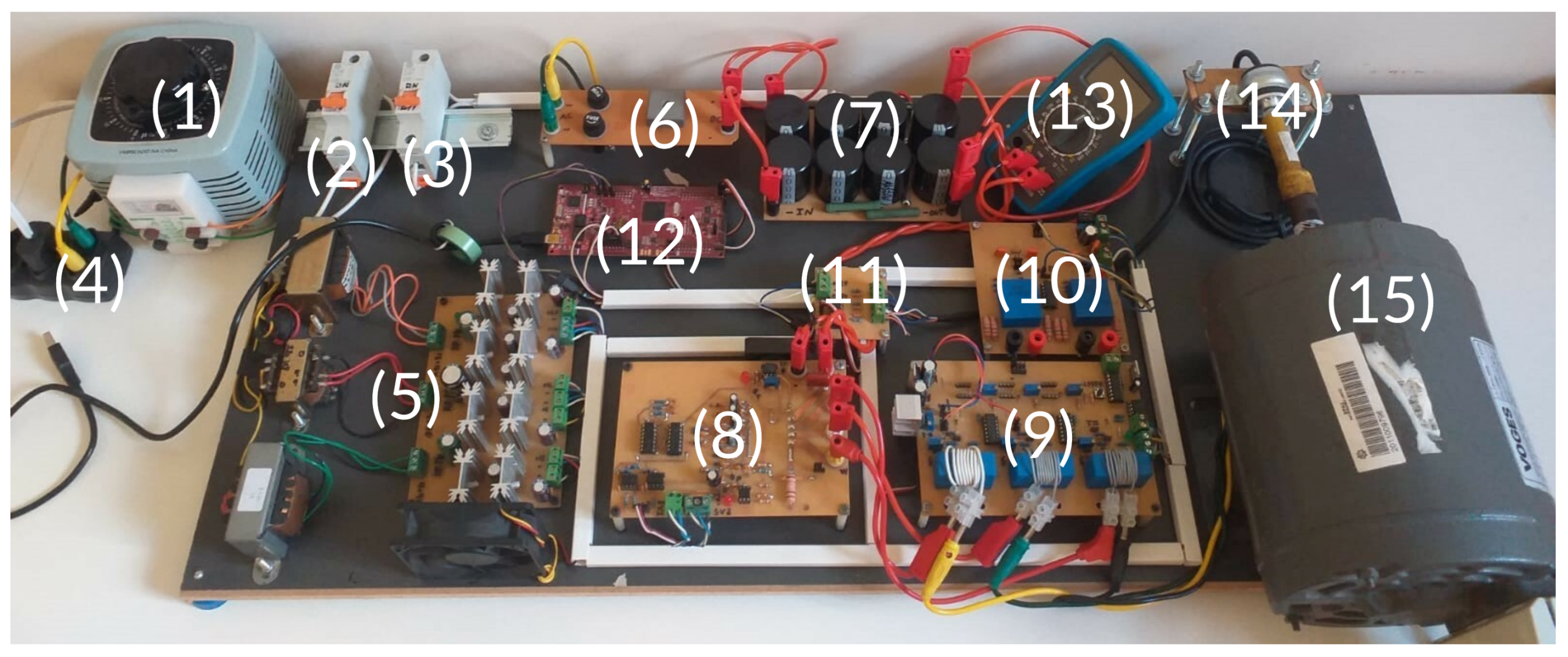
Figure 1 presents the system built to perform the experimental tests.
The experimental bench is composed of:
Variable auto transformer;
Auxiliary source power supply circuit breaker;
Circuit breaker of the capacitor bank pre-charge circuit;
AC power input;
Auxiliary voltage source;
Rectifier circuit;
DC link;
Three-phase inverter;
Current acquisition board;
Voltage acquisition board;
Encoder signal conditioning board;
TMS320F28379D DSP (Digital Signal Processor);
Digital multimeter;
Incremental encoder;
Three-phase induction motor.
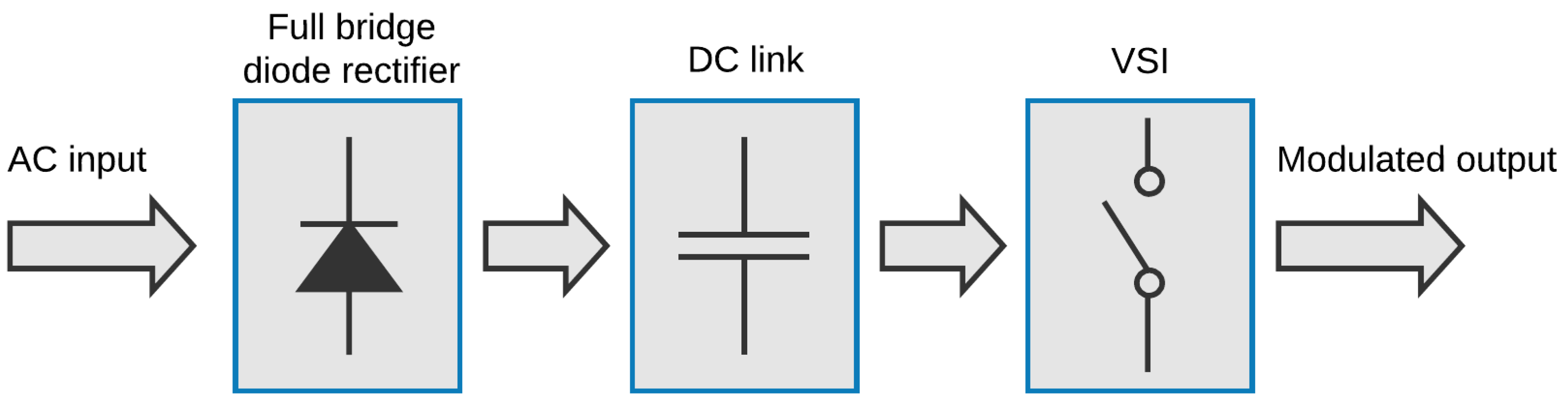
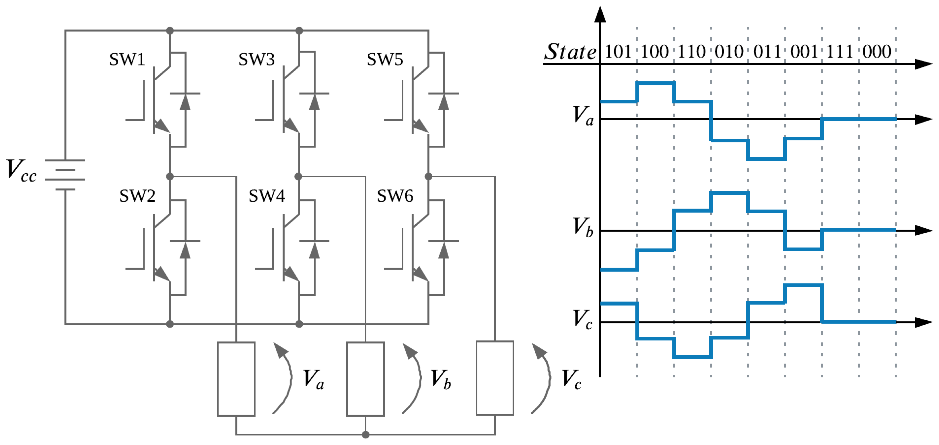
There are two basic types of inverters, Voltage Source Inverter (VSI), powered by a voltage source, and Current Source Inverters (CSI) powered by a current source. VSI topology is more common and synthesizes a well-defined voltage in the machine terminals while CSI provides a current signal in the machine terminals [
5].
Figure 2 presents the simplified schematic diagram of a VSI. This setting uses a rectifier to transform the AC input signal into DC. After rectification, the signal is filtered by the DC link to obtain a signal without oscillations. Next, the DC signal is applied to the three-phase IGBT bridge with the sole purpose of creating an alternating signal at the output by switching the semiconductor frequently defined by the modulation technique employed.
2.1. Digital Signal Processor
The TMS320F28379D microcontroller is designed for application in control systems, drive drivers, signal detection and processing. The DSP has two Central Processing Units (CPU), two Control Law Accelerator (CLA) and a maximum adjustable clock of 200 MHz [
25,
26].
LaunchPad features 32-bit architecture, 1 MB of flash memory, 204 kB of RAM, 14 analog-to-digital conversion channels (ADC) with 16/12-bit resolution and 14 channels designated for PWM function [
25,
27,
28].
2.2. Rectifier
Rectifiers can be classified according to the number of phases of the input AC voltage source, i.e., single-phase or three-phase. Depending on the semiconductors used, they can be classified as uncontrolled, semi-controlled, or fully controlled. Also, concerning topology, they can be classified as half-wave or full-wave rectifiers [
29]. The three-phase uncontrolled full-wave rectifier topology is common in converter drive applications because it uses diodes as the rectifying element, connected in a full-bridge arrangement.
In this configuration, the entire cycle of the alternating voltage of the power supply is rectified, providing in the voltage output a constant average value and with smaller oscillations [
29]. For this work, the full-wave bridge rectifier configuration encapsulated in the KBPC3510 IC is used. This rectifier allows a maximum current of 10 A, enough to supply the consumption of the three-phase induction motor used.
2.3. DC Link
The design of the DC link capacitors considers the power of the converter load, the maximum permissible voltage variation, and the hold-up time of the load, which is defined as the time that the output voltage should remain constant in the event of a momentary fault in the capacitor bank’s input voltage. The Equation (
1) is used to design the capacitor bank, given by
where
,
,
represent the rated power, hold-up time, and rated feed voltage of the machine, respectively. The variation of the output voltage was defined at 10% and the hold-up time of 8.33 ms, that is, a half cycle of the nominal frequency of the load. Thus, the capacitance value of the projected DC link is 4.4 mF, in which a total of eight EPCOS B43845 capacitors of 2200
F and voltage of 200
were used. The designed DC link can work with voltages up to 400
, enabling AC voltage connection at the rectifier input of 127
or 220
.
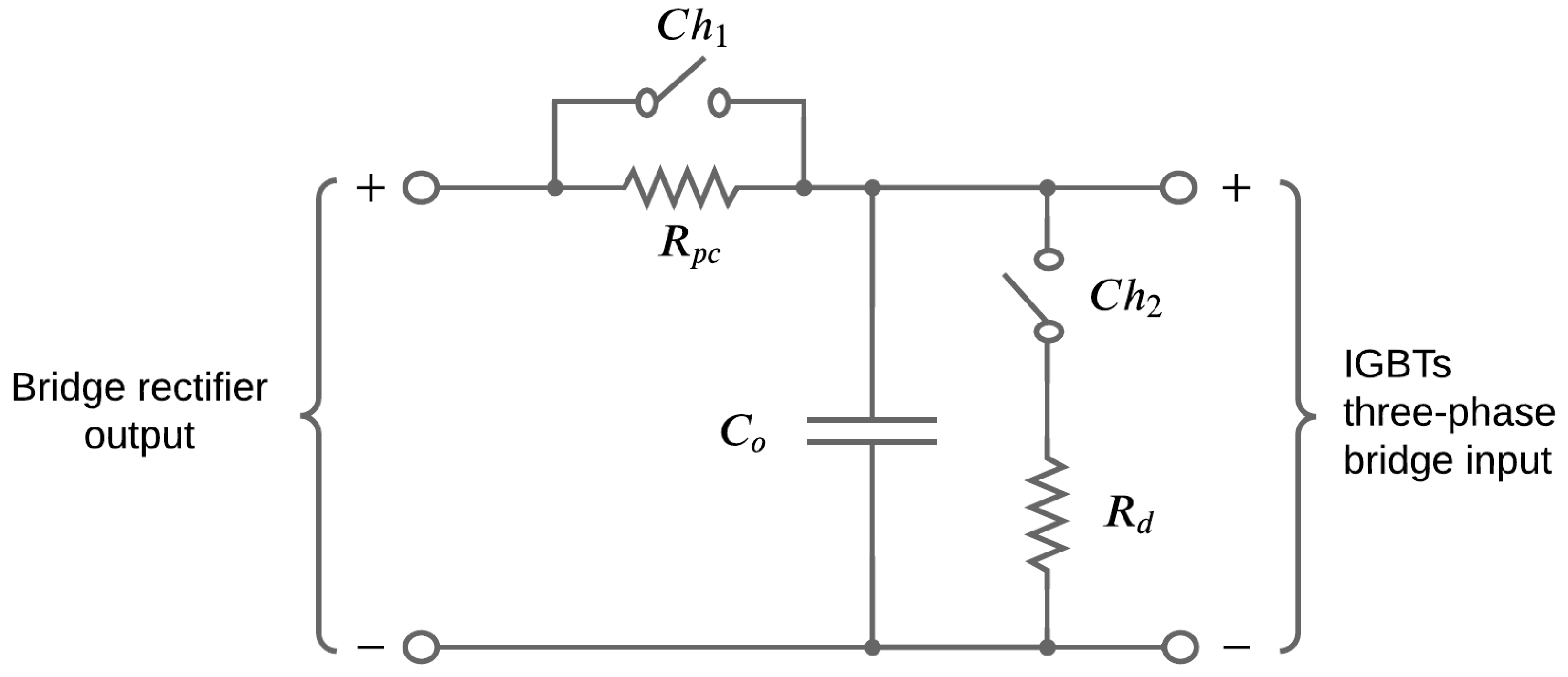
The DC link also contains pre-charge and bank discharge resistors. The pre-charge resistor is responsible for preventing a high in-rush current from flowing through the converter elements and damaging the components when the rectifier’s AC supply circuit breaker is tripped. The single-phase variable autotransformer at the input of the rectifier circuit was also employed for this purpose, allowing the input AC voltage to rise gradually to the value of 220 .
The discharge resistor has the function of draining the energy stored in the capacitors when the converter is switched off, ensuring that the voltage reduces to zero slowly, also avoiding accidents. Another function of the discharge resistor is to work as a braking resistor when the machine starts to work as a generator due to the type of load it drives. In this context, the DC link voltage tends to rise due to the reverse power flow.
Figure 3 illustrates the simplified DC link circuit with the pre-charge (
) and discharge (
) resistors.
The AC voltage at the input of the rectifier circuit is 220 . Thus, the DC voltage at the output of the rectifier corresponds to the maximum value of the input voltage, i.e., 311 . The pre-charge resistor was chosen so that the link voltage reaches the maximum value (311 ) in 5 s, while the discharge resistor was chosen so that the bank voltage is zero in 132 s. The switch is open only at the beginning of bank charging, and after the bank voltage stabilizes the switch is closed since the pre-charge resistor is no longer needed. Similarly, the switch () is closed when the converter is switched off, allowing the stored energy in the bank to be drained, and when in the normal operation of the converter, is open.
2.4. Power Module
The choice of Fairchild Semiconductor’s FNA41560 driver is a consequence of the need for a compact and high-performance solution for the frequency inverter. The chip features optimized circuit protection and a combined IGBT drive to reduce losses. The module is also equipped with overcurrent protection, under-voltage interlocks, temperature monitoring output, bootstrap diodes and features gate drive circuits and internal dead-time.
The FNA41560 must be powered with a voltage of 15
, supports 600
(drain-source voltage) in the IGBT while dissipating 41 W of power in each semiconductor. The module operates with a maximum switching frequency of 20 kHz, a maximum current of 15 A at 25 °C, an insulation rating of 2000
/min and terminals for individual current monitoring of each phase [
31].
The power module has six PWM outputs to drive the IGBTs, which can be controlled by the DSP via optocoupler ICs. The PWM modules of the DSP have complementary outputs and internal dead-time production. However, a gate drive circuit was designed to receive the command signals from the upper switches of the three-phase IGBT bridge and, from these, the command signals of the lower switches and the dead-time between the switches of the same arm are produced via hardware. In this way, configuration errors of the PWM channels and dead-time of the DSP that could damage the FNA41560 are avoided.
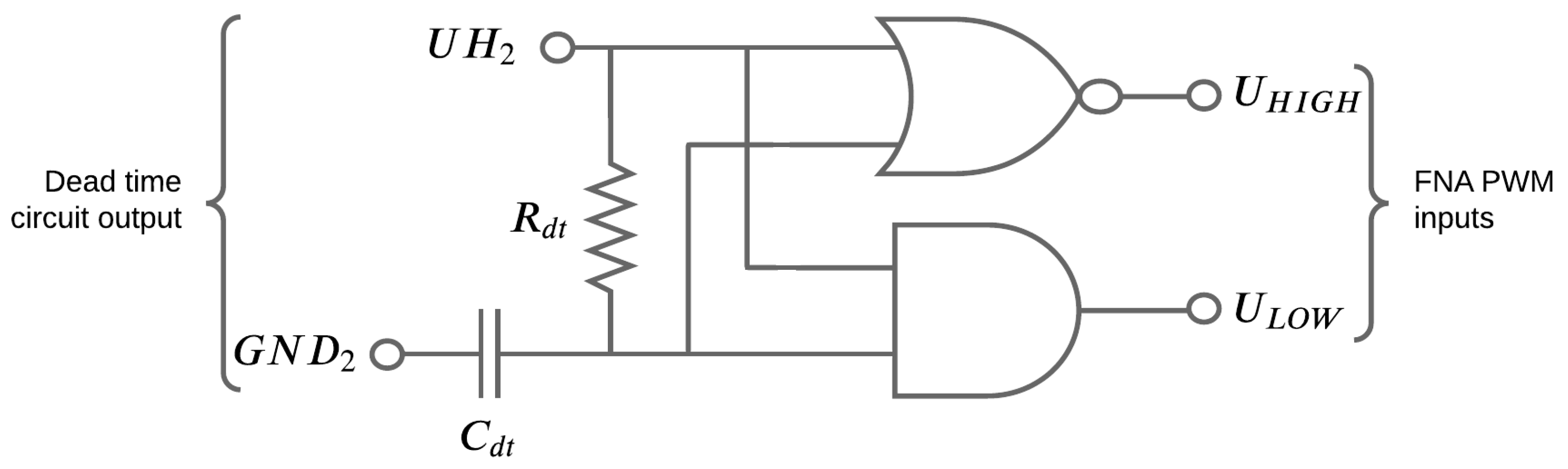
Figure 4 illustrates the dead-time generation circuit for the U-arm of the three-phase IGBT bridge.
From
Figure 4 it is noted that the circuit to generate the complementary signals has a resistor (
) and a capacitor (
) to generate the dead-time between the switches of the same arm along with AND and NOR logic gates. The switching frequency chosen is 10 kHz, within the operating range of the FNA41560. Thus, the resistor and capacitor were set to guarantee a dead-time of 1
s equivalent to 1% of the switching period.
The designed PCB of the IGBT module contains three dead-time generation circuits and complementary signals. Looking at
Figure 4, when applying a high logic level signal to the
input of the first arm, the
output also assumes high logic level. However, the
output, which drives the lower IGBT, has a low logic level with the addition of the time delay, preventing simultaneous driving of the switches. The same principle is extended to the switches of the V and W arms of the three-phase IGBT bridge.
In addition, to drive the module’s switches, optical isolation circuits or optocoupler circuits were used. These are circuits used with the purpose of electrical decoupling, the PWM channels of the DSP do not have a direct electrical connection with the inputs of the FNA41560. Its working principle is based on a Light Emitting Diode (LED) that, when energized, emits a light that puts a phototransistor in a conduction state [
32].
The necessity for electrical isolation comes from the fact that there are voltages and currents in the power stage that could cause damage to the control and data acquisition circuits. For this reason, the reference of the power module is different from the reference of the DSP and the data acquisition boards, ensuring the isolation of the control and measurement circuits from the power circuits.
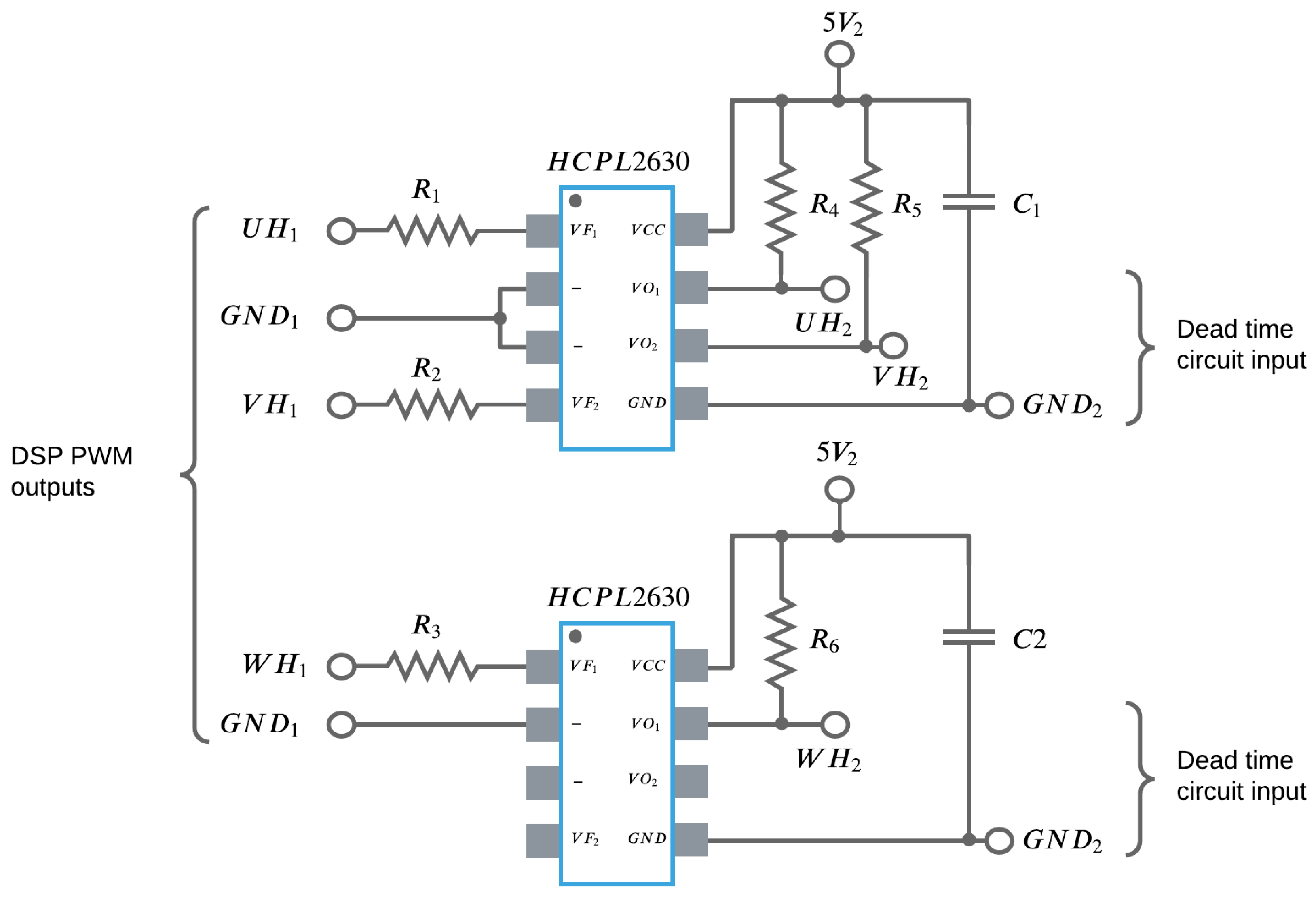
For this project, it was chosen to use optocouplers of the HCPL2630 type. These ICs work with Transistor-Transistor Logic (TTL) logic level, considerable electrical isolation, 12 ns delay time and have two independent channels in the same encapsulation [
33].
Figure 5 illustrates the circuit developed to isolate PWM signals from the DSP to the FNA41560 driver.
The PWM signals coming from the DSP have as reference , while at the output of the optocouplers (power stage), the reference is . At the output of the isolation circuit, the PWM signals are injected into the dead-time circuits and there is the generation of the complementary PWM to drive the IGBTs of the power module.
To monitor the temperature of the power module, a voltage comparator circuit with a variable resistor was designed to adjust the maximum temperature limit of the FNA41560. The IGBT module has an internal thermistor that changes its resistance according to the temperature change. If the module temperature exceeds the set limit, the circuit containing the operational amplifier LM2904 changes the state of the output from logic level low to high. In this context, the signal at a logic high level triggers an LED as a visual alert, in addition to sending a pulse to the DSP to interrupt the PWM signals from the IGBTs.
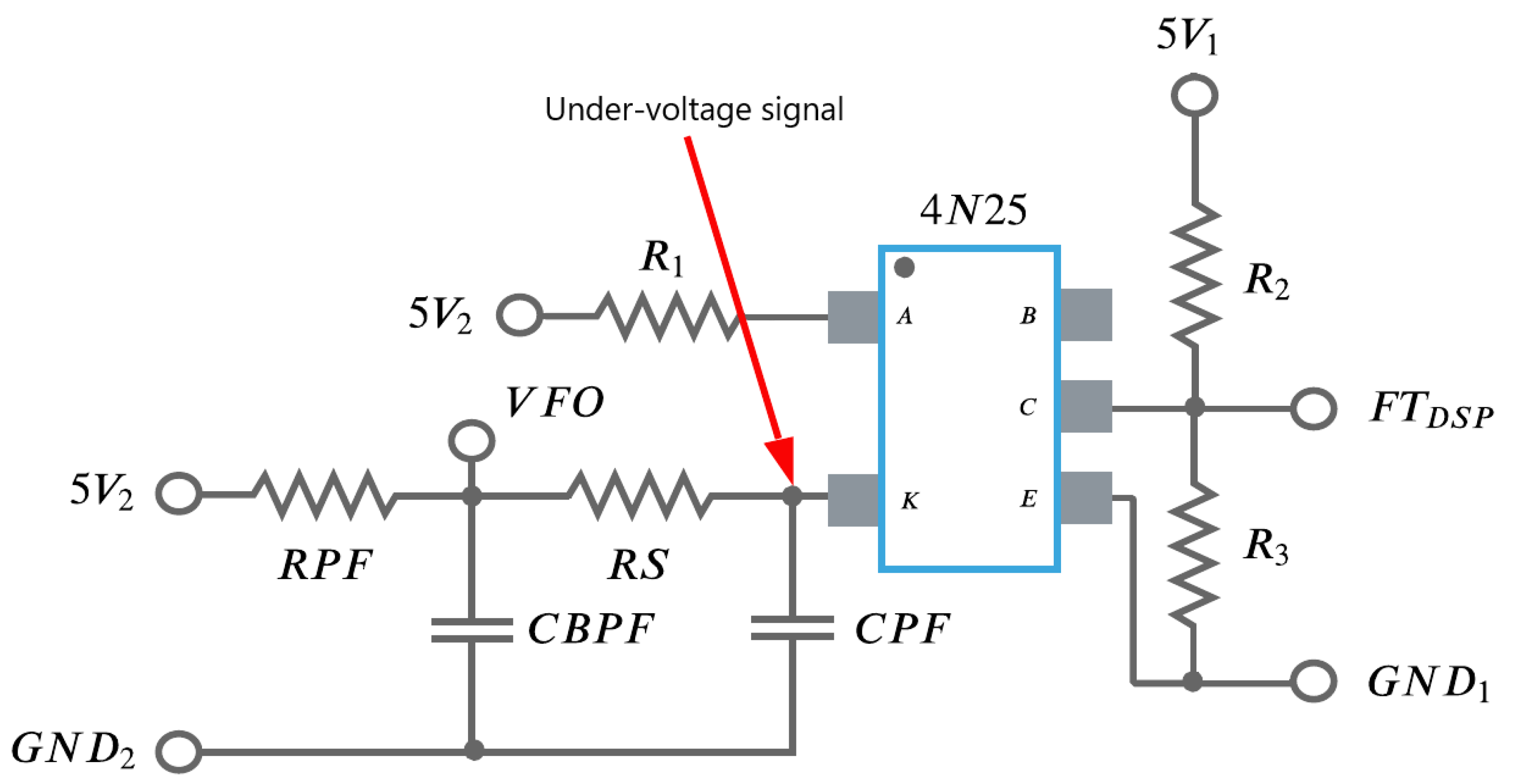
Figure 6 presents the circuit used for under-voltage blocking recommended by the FNA41560 manufacturer. Also, a 4N25 optocoupler and a voltage divider circuit were used to transmit the signal to the DSP.
The resistors RPF, RS and the capacitors CPF, CBPF are defined according to the module datasheet. The resistor is used to limit the current of the optocoupler LED, the resistors and are the voltage divider resistors. The values of 200 , 10 k and 20 k respectively have been set. The terminals “A” and “K” of the 4N24 IC indicate the Anode and Cathode terminals of the LED. The terminals “C”, “B” and “E” represents the collector, base and emitter terminals of the phototransistor, respectively.
Short-circuit current detection of the FNA41560 is provided by a shunt resistor located at the source terminals of the lower IGBTs of the three-phase bridge. If the voltage across the resistor exceeds the short-circuit threshold voltage trip level (0.5
) at the
input of the module, a fault signal is assigned and the lower arm IGBTs are turned off [
34].
The protection circuit contains a low-pass filter, formed by resistors and capacitor . The module manufacturer suggests values for these components in such a way that the time constant is between 1 s and 2 s. A 15 resistor and 100 nF capacitor were used, i.e., filter time constant of 1.5 s. A shunt resistor with a value of 0.1 was sized. Thus, for the protection to operate, a current greater than or equal to 5 A circulating through the module is required.
2.5. Current Measurement
The current measurement of the converter was made using the LA 55-P Hall-effect sensor from the LEM manufacturer.
Table 1 presents the characteristics of the transducer.
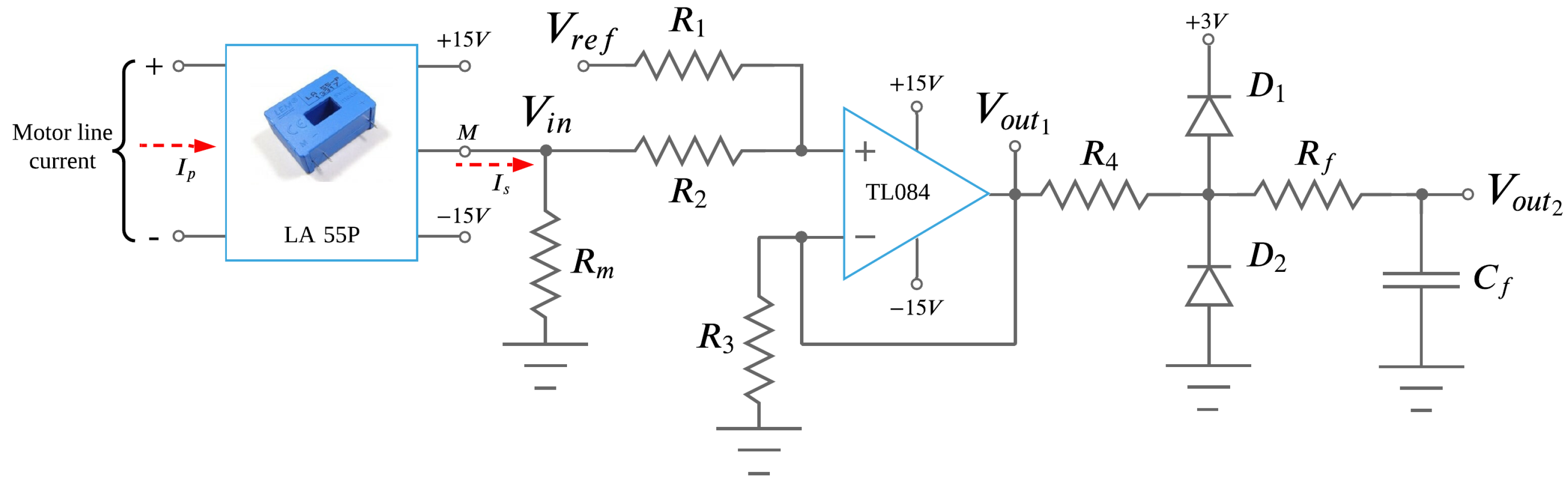
When an electrical current circulates through the primary winding (
) of the current sensor, a current also circulates in the secondary (
) proportional to the conversion ratio of the transducer. The current in the secondary in turn produces a voltage (
) on the shunt resistor
and thus this voltage signal is fed into the non-inverting adder circuit. In the design of the current acquisition circuit, it was chosen to use the TL084 operational amplifier and the
resistor was set to a value of 100
. The current conditioning circuit is shown in
Figure 7.
The voltage signal
is responsible for adding an offset voltage to the signal. Since the analog-to-digital conversion channels of the DSP operate with input voltages between 0 and 3
, an offset voltage must be added to the input signal such that this voltage represents the null measurements of the sensor, while voltages above the offset value represent positive measurements of the sensor and voltages below the offset voltage represent negative measurements. The Equation (
2) presents the relationship between output voltage
with inputs
and
, given by
Therefore, the output voltage is given by half of the reference voltage and half of the input voltage. The output signal of the non-inverting adder circuit passes through a clipper circuit, composed of two diodes and a resistor, whose function is to limit the output voltage of the operational amplifier between 0 and 3 .
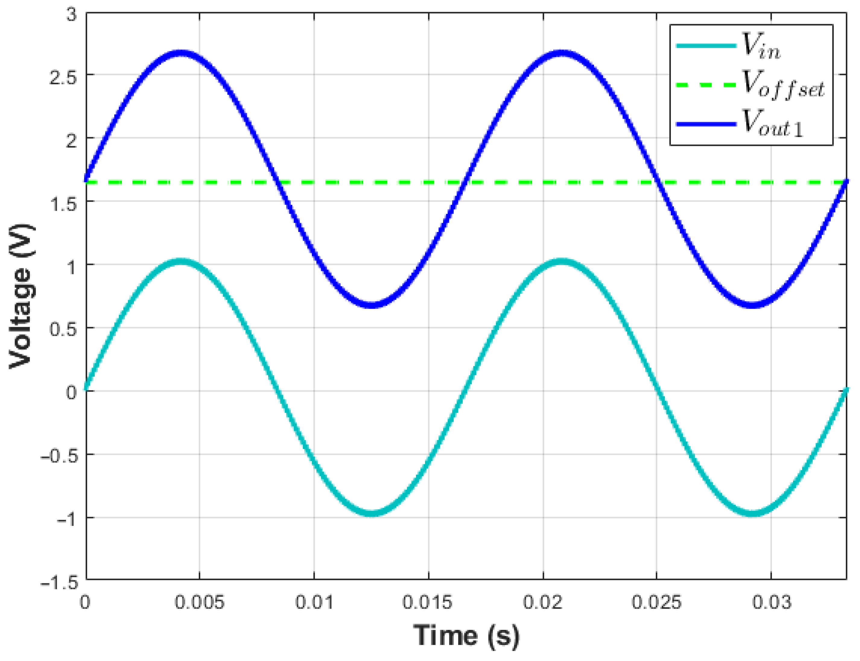
A simulation was developed to evaluate the operation of the current conditioning circuit. Considering a current in the secondary of the transducer of 10 mA and reference voltage of 3 , i.e., offset voltage of 1.65 to ensure that the post-processing signal remains in the middle of the reading range. In addition, a signal with a frequency of 10 kHz and amplitude of 0.05 V was added to the input signal to represent the noise present in the current measurement as a function of power module switching.
Figure 8 shows the result of the current conditioning circuit simulation.
By inspecting
Figure 8, it is possible note that the
voltage signal oscillates over the offset voltage value and remains between 0 and 3
. However, the voltage signal representing the current is not exclusively sinusoidal, it contains a high-frequency component, coming from the switching of the power module. Thus, it is desirable to remove the ripple caused by switching. The RC loop consisting of
and
, operating as a passive anti-aliasing low-pass filter was inserted into the output of the conditioning circuit, as presented in
Figure 7. The Equation (
3) is used to calculate the filter cutoff frequency, given by
A cutoff frequency of 2.4 kHz was adopted for the filter and, thus, the value of the resistor used was 2 k
and the capacitor of 33 nF.
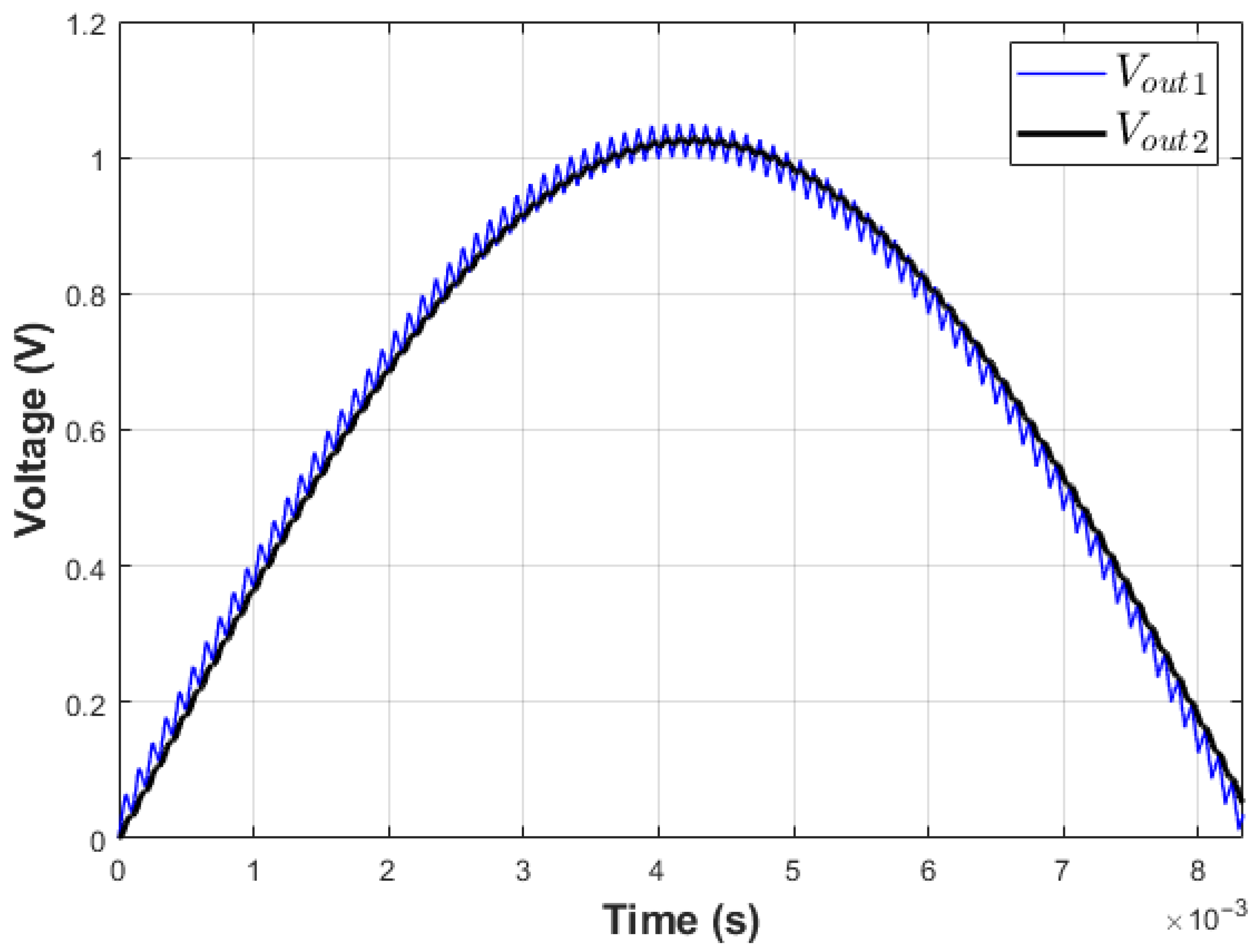
Figure 9 shows the comparison between the input voltage signal and the voltage signal after the low-pass filter.
From
Figure 9 it is noted that the ripple caused by switching has been considerably attenuated by the filter used. It can also be seen that a delay has been incorporated into the signal, but not very significantly.
2.6. Voltage Measurement
The LV 20-P voltage transducer from the manufacturer LEM was used for voltage measurement.
Table 2 shows the characteristics of the sensor.
When applying a voltage to the sensor measuring terminals, a current () is produced in the primary winding. Thus, in the secondary, the current () is produced due to the transducer conversion ratio. In turn, the current in the secondary produces a voltage on the shunt resistor () which reflects the voltage applied to the primary of the sensor.
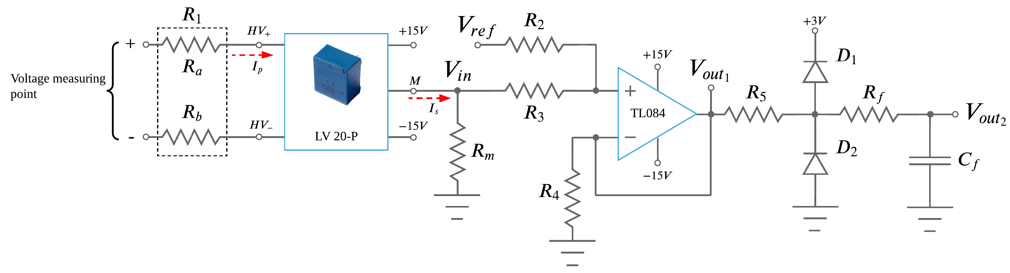
The voltage conditioning circuit is like the current conditioning circuit, shown in
Figure 10.
From
Figure 10 it is noted the presence of resistors on the primary side of the voltage sensor. The function of this resistor is to limit the transducer primary current according to the information presented in
Table 2. Thus, it was adopted for the
resistor a value of 75 k
, enabling the measurement of voltages up to 500 V. For the shunt resistor
a value of 100
was adopted.
2.7. Measurement of Rotor Position and Speed
The measurement of the machine’s speed, position and direction of rotation can be accomplished through the encoder. The encoder used, called incremental with quadrature output, is a device capable of converting shaft rotation information into pulse train signals. State-of-the-art encoders mostly operate on potentiometric, capacitive, magnetic, or optical principles [
37].
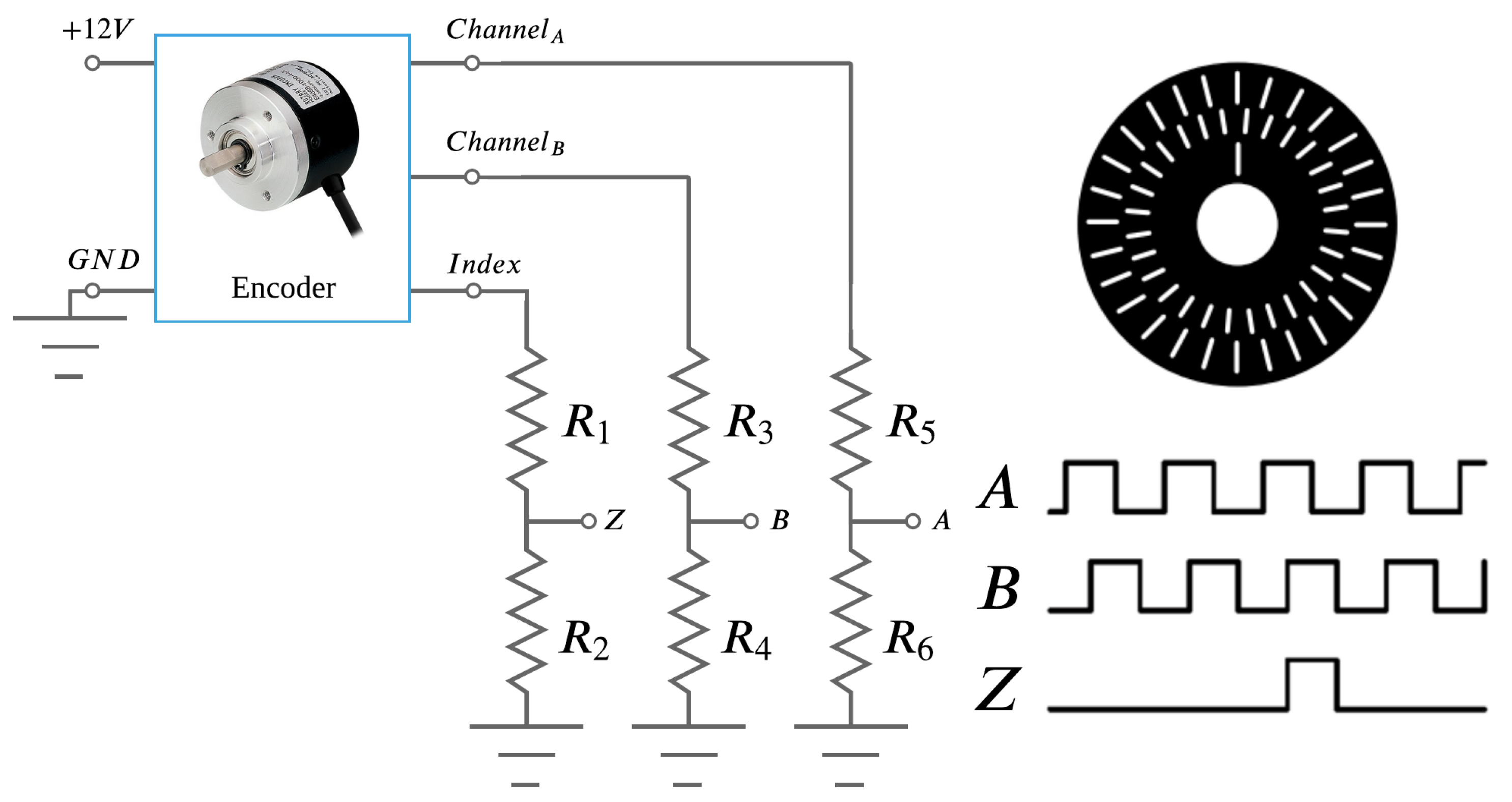
The incremental encoder is composed of a disk with a series of slots, an infrared light source, and a photoelectric sensor that produce the electrical pulses of channel A. The direction of rotation is obtained by the second strip of slots, channel B, positioned such that they produce an electrical 90
lag concerning channel A. The frequency of the pulse train of channels A and B are directly proportional to the rotational speed of the machine’s rotor. The third channel (index) outputs a high logic level signal with each complete revolution of the encoder disk.
Figure 11 shows the encoder conditioning circuit and the pulse train of each output channel.
The output voltage of the channels is , as a function of the encoder supply which is . To connect these signals to the DSP’s eQEP (Enhanced Quadrature Encoder Pulse) inputs, voltage divider circuits were used to reduce the voltage of the three output channels. In addition, operational amplifiers were used in the voltage buffer configuration, isolating the input signal from the DSP.
The encoder model used for the development of this work is the E30S4 and has an output with a resolution of 360 pulses per revolution.
2.8. Auxiliary Voltage Source
The auxiliary voltage source has multiple outputs: ±15 , ±12 , 5 and 3.3 . These voltages are required to power the integrated circuits and sensors of the current measurement boards, voltage measurement, encoder, and complementary power driver circuits. It is also important to mention the need to use voltage sources isolated concerning the sources that power the power driver, to prevent short circuits in the power step damage the inverter measurement and control circuits.
2.9. Induction Motor Parameters
For the experiments, an induction motor from the manufacturer Voges was used.
Table 3 shows the electrical and mechanical parameters of the machine.
Some parameters were collected directly from the motor board data and others were obtained through the blocked-rotor and no-load tests.
3. Dynamic Modeling of the Indirect Field Oriented for the MIT
The field-oriented control strategy is classified according to the method of acquisition of the rotor flux angle. In the direct method (Direct Field Oriented Control—DFOC), sensors installed in the machine’s air gap are used to measure the flux. In the indirect method (IFOC), there is no flux measurement, the position and slip are used to obtain the position of the rotor flux angle [
5].
The IFOC makes use of the fact that satisfying the relationship between slipping and stator current is a necessary and sufficient condition to produce field orientation [
5].
In Field Oriented Control (FOC), one can make a direct analogy with the field-independent DC machine control [
38]. In DC machines, the magnetic flux established by the armature and field currents is orthogonal to each other, regardless of the rotor’s position and mechanical load. Thus, for a constant field current level, the armature current is responsible for the machine’s torque production. In asynchronous machine FOC, the same principle applies, where the direct axis current is responsible to establish the machine’s magnetic flux and quadrature axis current is responsible for the torque level.
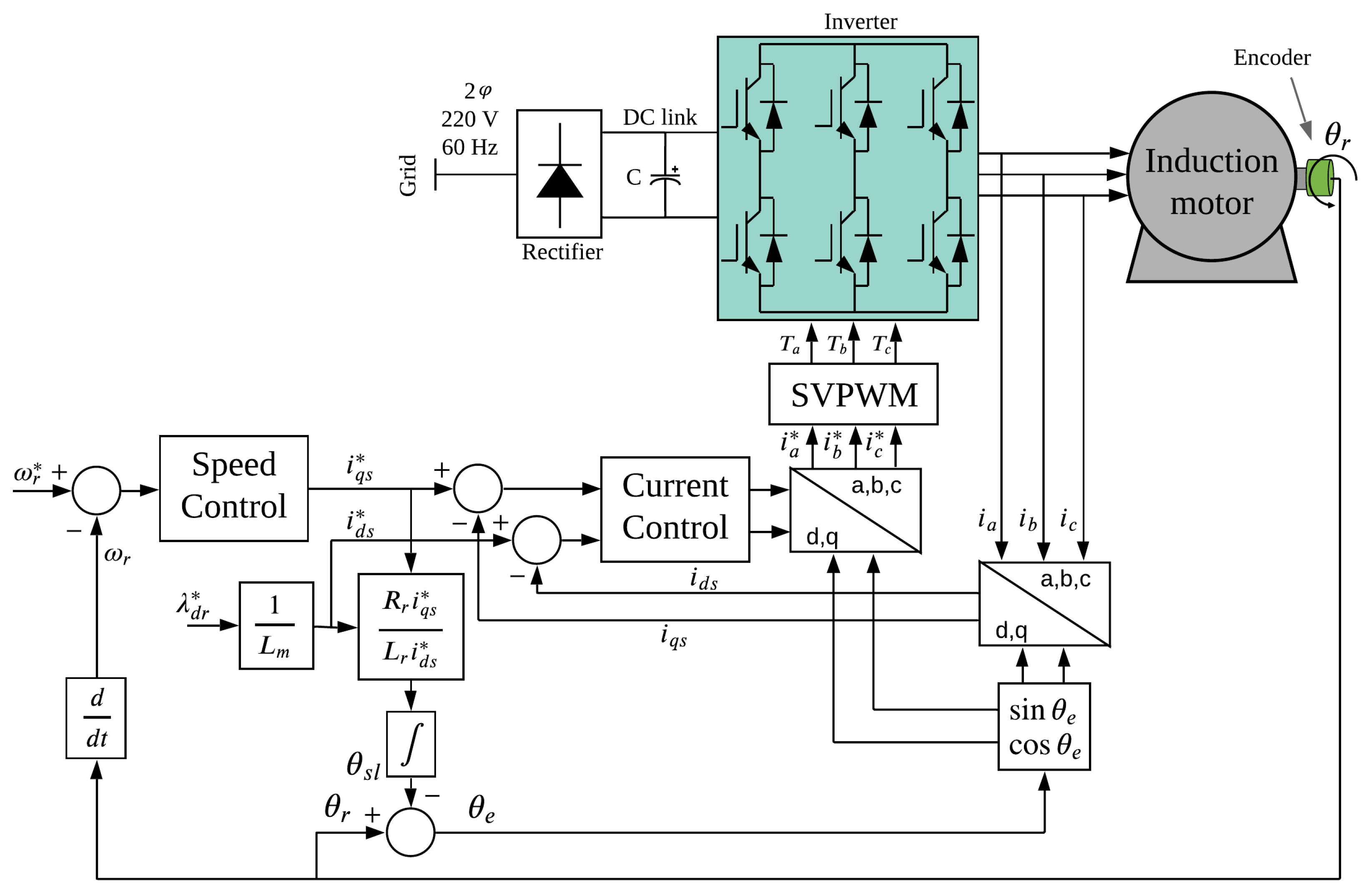
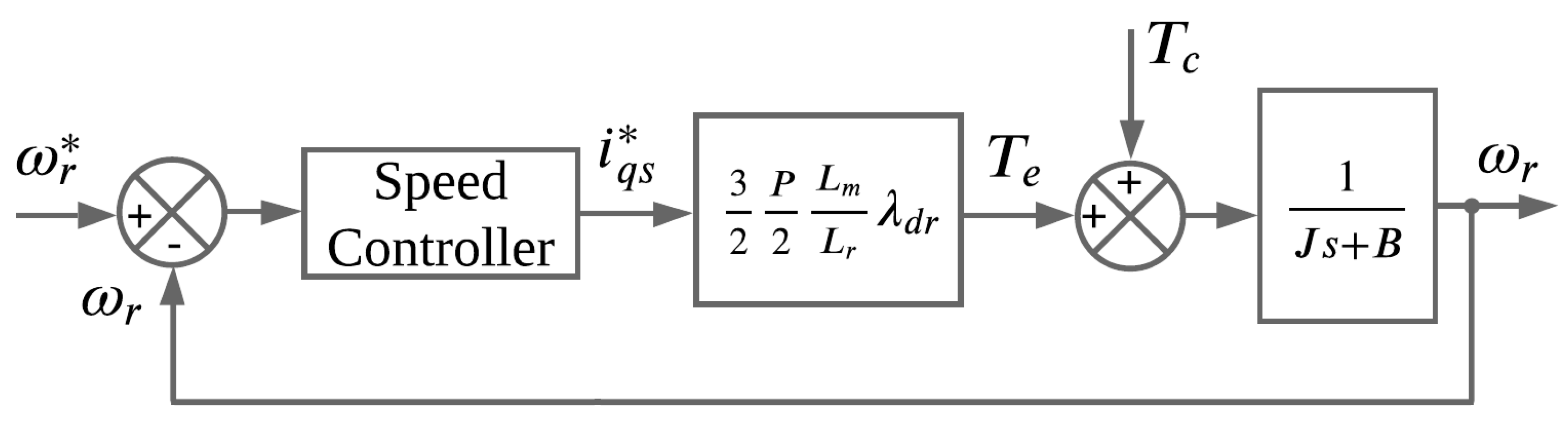
Figure 12 presents the block diagram of the proposed speed control system using the indirect oriented field control strategy for the three-phase induction machine [
39]. The system consists of an induction motor with a three-phase inverter, SVPWM modulation block, orientation block in which the rotor flux angle is calculated, block for the referential transformations (ABC to dq0) through Clarke and Park transformations, current control loop, speed control loop and position control loop. In this paper, only the design and tuning of the current and speed control loops will be addressed.
The equation of the dynamic model of the induction machine with indirect orientation presented in this paper is supported on the models and simplifications described in [
5,
39,
40].
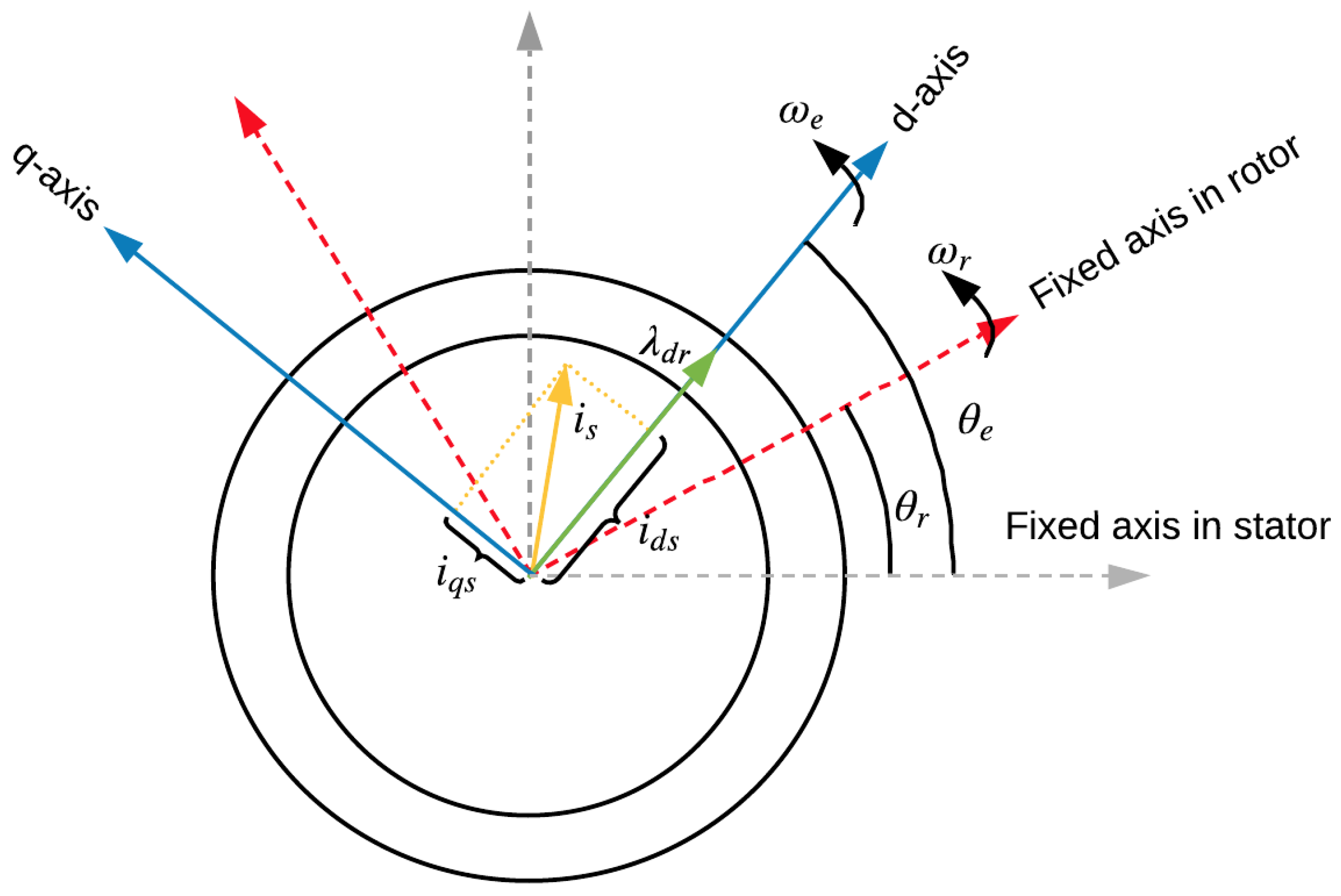
In an ideal field oriented of a three-phase induction machine, there is decoupling between the direct and quadrature axes, and the rotor flux is aligned to the direct axis (
Figure 13). Thus, the flux and its derivative on the quadrature axis are null.
Thus, the Equation (
4) is used to calculate the rotor flux, given by
where
,
,
and
represent mutual inductance, rotor inductance, rotor resistance, direct axis current, and
p represents the derivative in time (
), respectively.
The equation of the electromagnetic torque (Equation (
5)) can be found considering that the electrical time constant of the system is negligible concerning the mechanical constant in the Equation (
4), thus, it is obtained
where
is the electromagnetic torque,
P are the number of poles,
the direct axis flux and
the quadrature axis current that denotes the torque command of the machine. The Equation (
6) shows that the direct axis current is directly related to the magnetizing current of the machine, given by
In the indirect field-oriented method, the frequency needs to be calculated in dq0 coordinates. Thus, the Equation (
7), allows obtaining the slip frequency, given by
The Equation (
8) relates the torque, rotor velocity and angular position, given by
where
,
J,
B and
denote the rotor position, moment of inertia, viscous coefficient of friction and load torque, respectively.
4. Space Vector Pulse Width Modulation—SVPWM
The SVPWM is a modulation technique that presents reduced switching number and allows better utilization of DC link voltage, compared to the SPWM (Sinusoidal Pulse Width Modutalion), widely used in scalar V/F AC drives. In addition, the SVPWM presents reduced current harmonic distortion and relatively simple digital implementation [
3,
41,
42,
43].
Figure 14 presents the waveforms of the eight possible states for a two-level three-phase inverter. Furthermore, it is considered that at the instant when the upper switch of one arm of the converter is closed, the lower one is open and reciprocal.
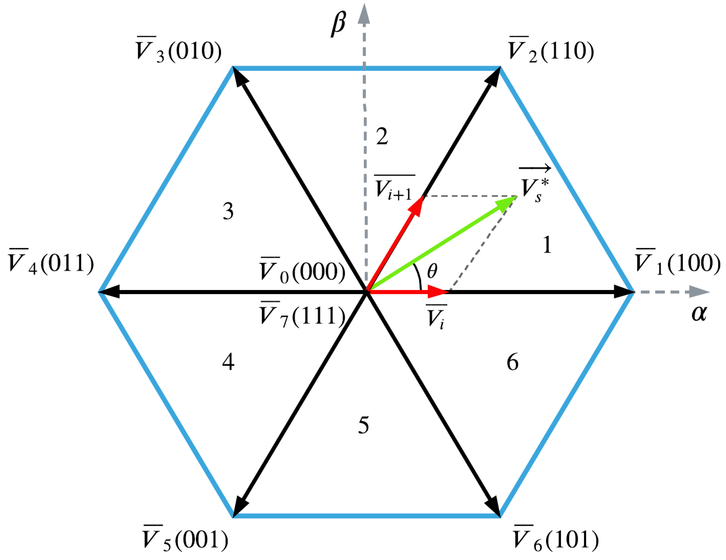
Each of the six nonzero states gives rise to a vector in the complex plane
(
Figure 15). The six active vectors have magnitude
and lagged from each other by an angle of 60°. The null vectors are represented at the origin of the complex plane.
To synthesize a reference voltage level (
) during a sampling time interval (
) it is necessary to use adjacent voltage vectors and null vectors. The Equation (
9) is used to calculate the reference voltage, given by
where
and
are adjacent vectors,
and
null vectors,
,
correspond to the length of time adjacent vectors are used, while
and
represent the duration of null vectors. The Equations (
10)–(
12) allow you to calculate the duration times of adjacent and null vectors, given by
To avoid over-modulation in SVPWM modulation, the amplitude of the reference vector cannot be larger than the magnitude of the largest circumscribed radius of the hexagon. In SPWM the use of the DC link voltage is restricted to
. In, SVPWM the maximum magnitude of the voltage reference is
, i.e., 15% increase in the utilization of the voltage available on the DC link [
44,
45].
6. Results
To analyze the behavior of control loops and vector control strategy, simulations were performed in the MATLAB/Simulink® software. Subsequently, the same tests were performed on the commissioned converter prototype. In this way, it is possible to examine the behavior of the converter both with regard to hardware operation and the practical implementation of the field-oriented control strategy on a real machine.
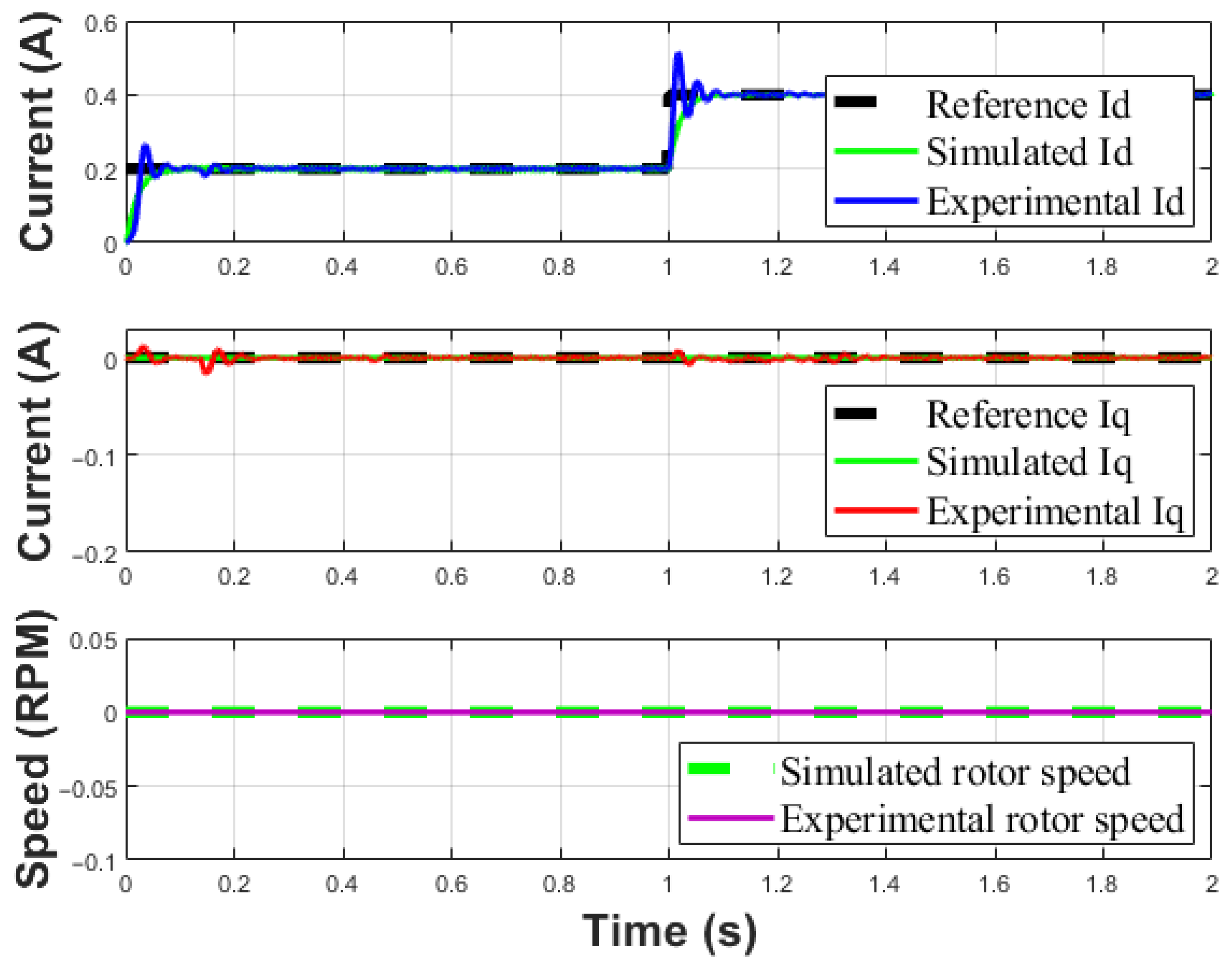
Initially, reference profiles were applied only to the direct axis current loop to evaluate the magnetization of the machine.
Figure 18 presents the behavior of the direct axis loop for references of
A and
A. In addition, the bottom part shows the rotor speed of the machine.
It is verified in
Figure 18 that the controller can keep the currents at the reference values. Furthermore, it is possible to analyze the behavior of the rotor speed, which due to the presence of only magnetizing current, the rotor stands still.
Table 6 presents the performance results of the direct axis current controller.
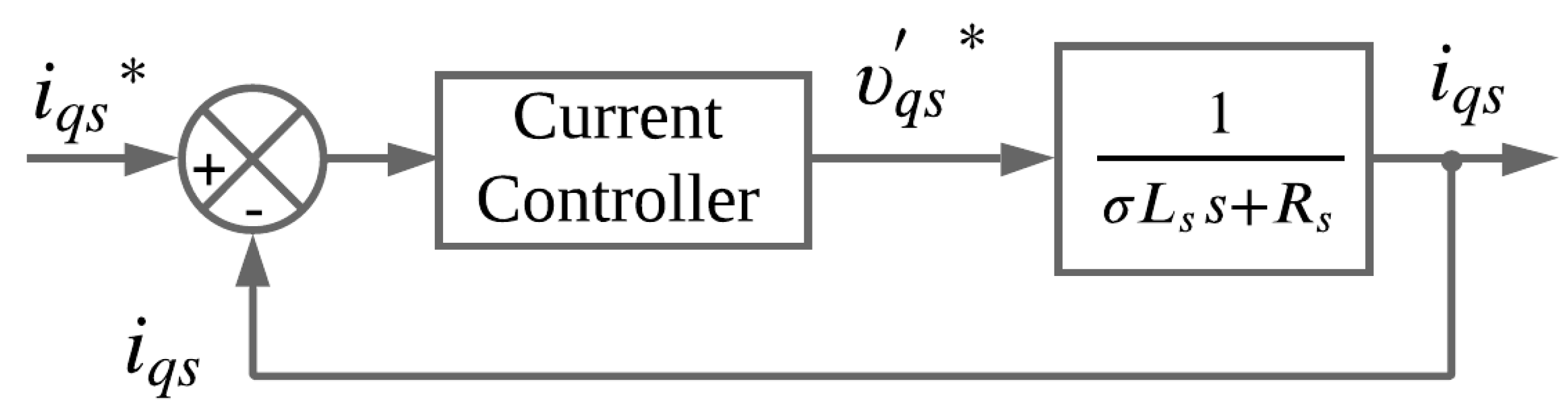
The overshoot present in the experimental signal is related to simplifications adopted for the current controller design. The closed-loop transfer function of the current plant presents a zero. This zero was disregarded to calculate the PI controller gains. Thus, in the real system, this zero will cause a proportional overshoot for fast responses, but the settling time will be preserved.
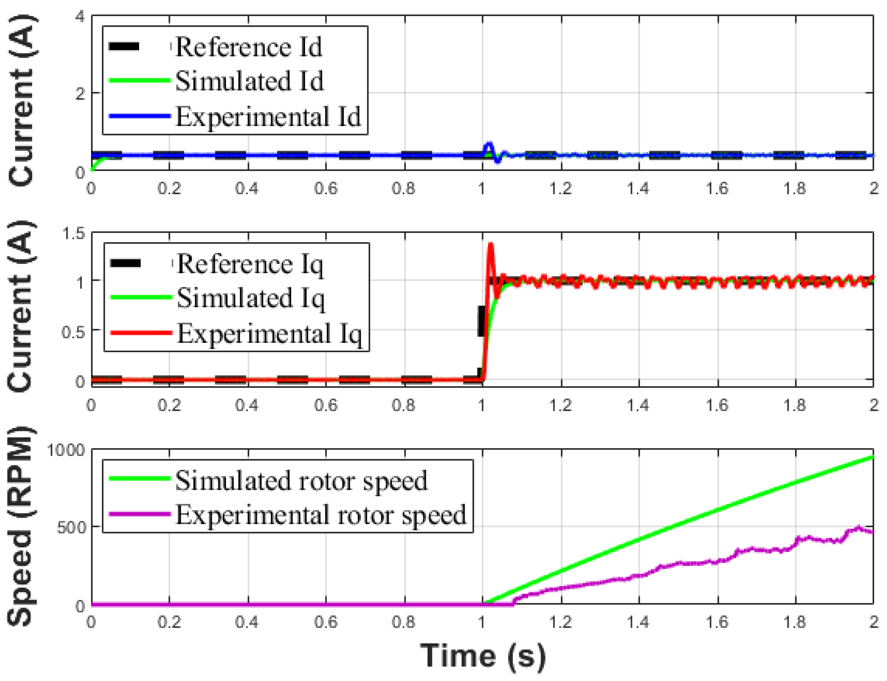
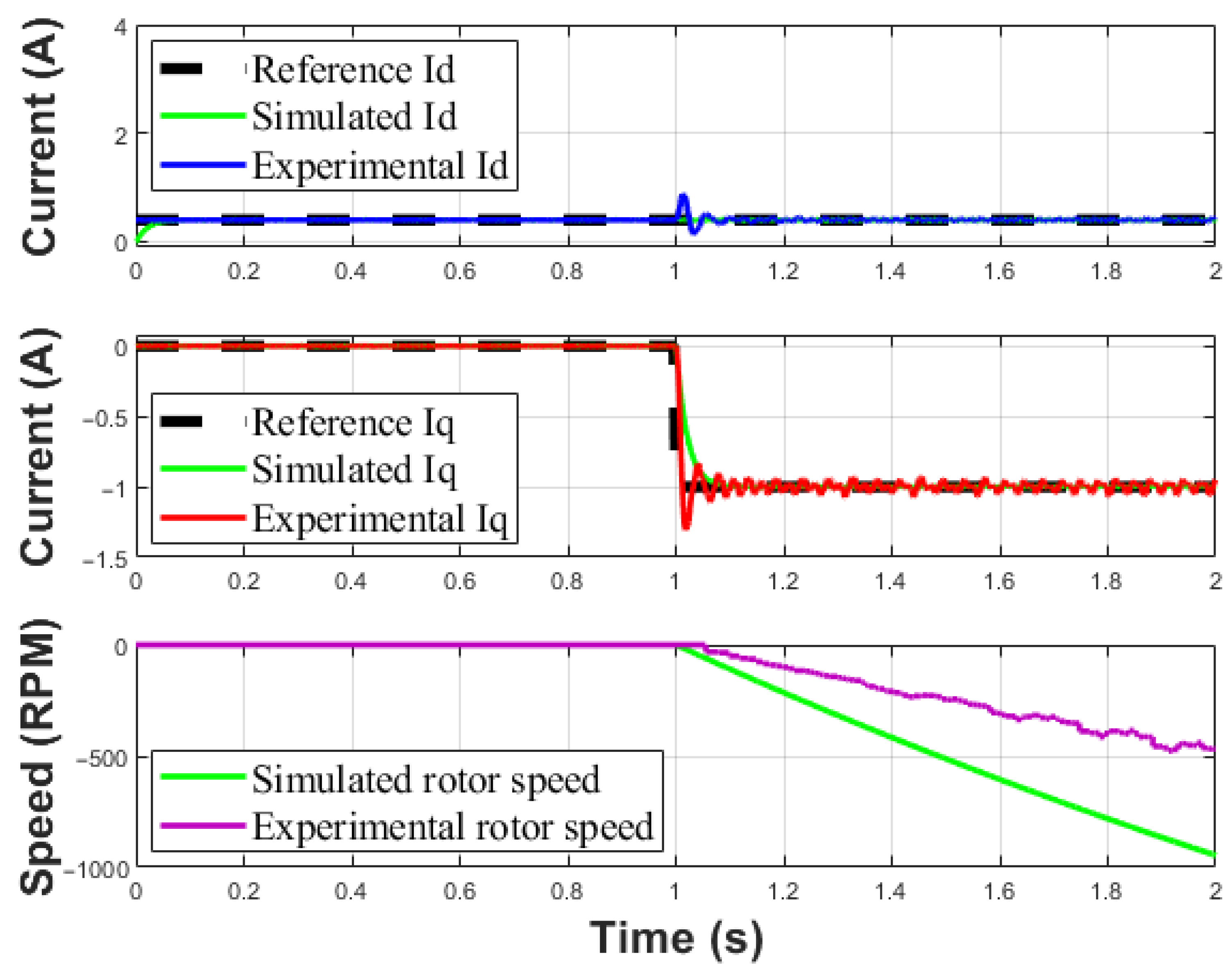
To verify the behavior of the quadrature axis current controller, reference profiles were applied in positive step of 1.0 A and negative step of −1.0 A, as shown in
Figure 19 and
Figure 20, respectively.
Analyzing the
Figure 19 and
Figure 20, the controller can maintain the imposed references. Still, it is possible to highlight that for positive current values in the quadrature axis, the machine rotor rotates clockwise. However, for negative values of current in the quadrature axis, the machine rotation is reversed, characterized by negative speed values.
For both situations, the speed of the machine increases wildly, because there is no speed control loop. It is also noted that the speed of the machine in simulation assumes higher values than those collected in the experiments. The explanation for this is since in simulation many electrical and mechanical elements are considered ideal or even not present in the machine model. Thus, they do not contribute to the speed behavior of the machine. In the same way as clarified for the current , the overshoot of the current control loop is justified.
Table 7 presents the performance parameters of the quadrature axis current controller.
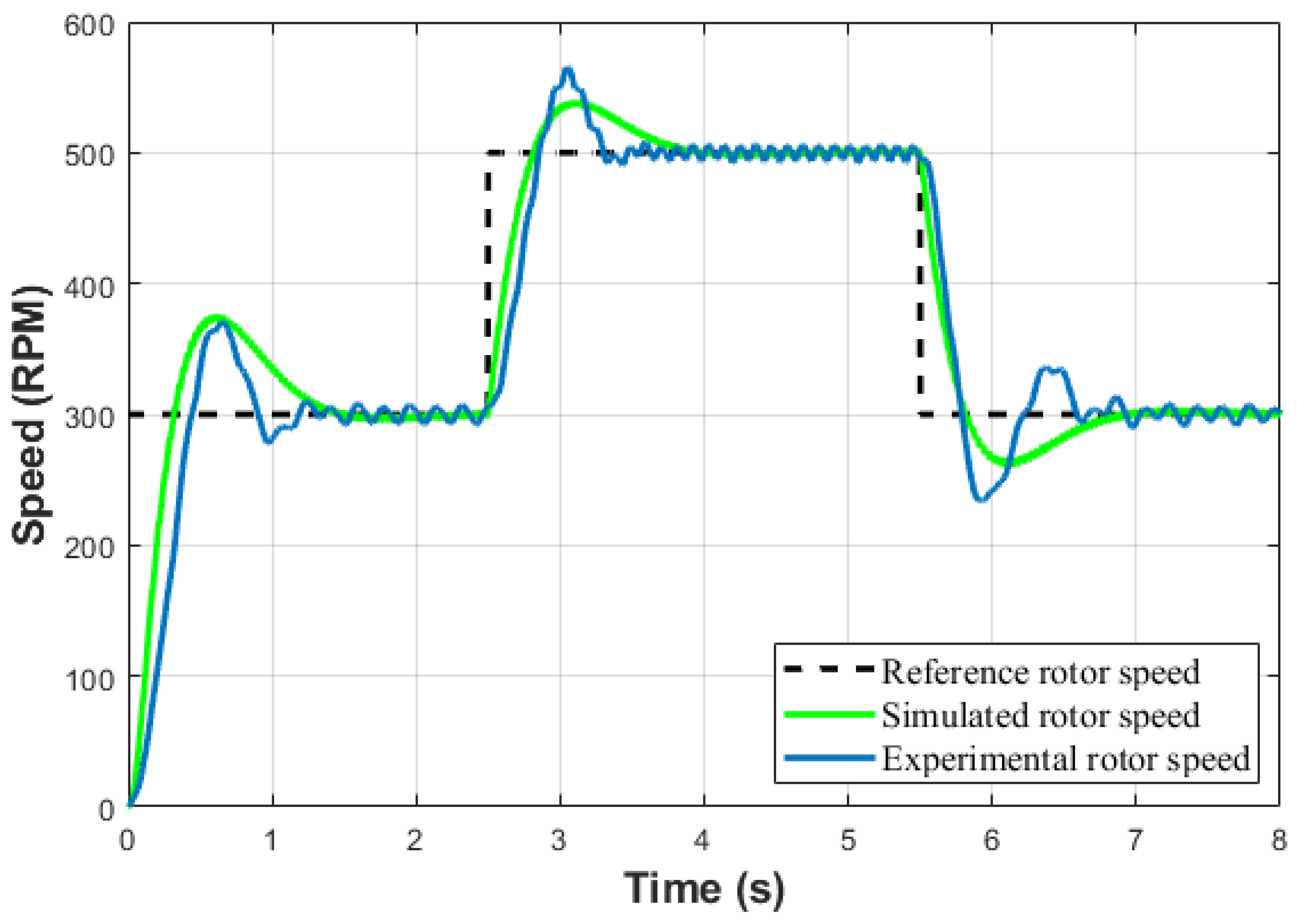
After validating the correct operation of the current control loop, the speed control loop controller was simulated and implemented in the digital signal processor. The direct axis current reference was set at a value of 0.4 A, which represents the magnetization of the machine, and experimentally was the value that presented the best speed and torque results. Tests were performed with step, trapezoidal, and sinusoidal references. For a positive step reference, initially with a reference of 300 RPM and then increasing to 500 RPM and returning to 300 RPM, as shown in
Figure 21.
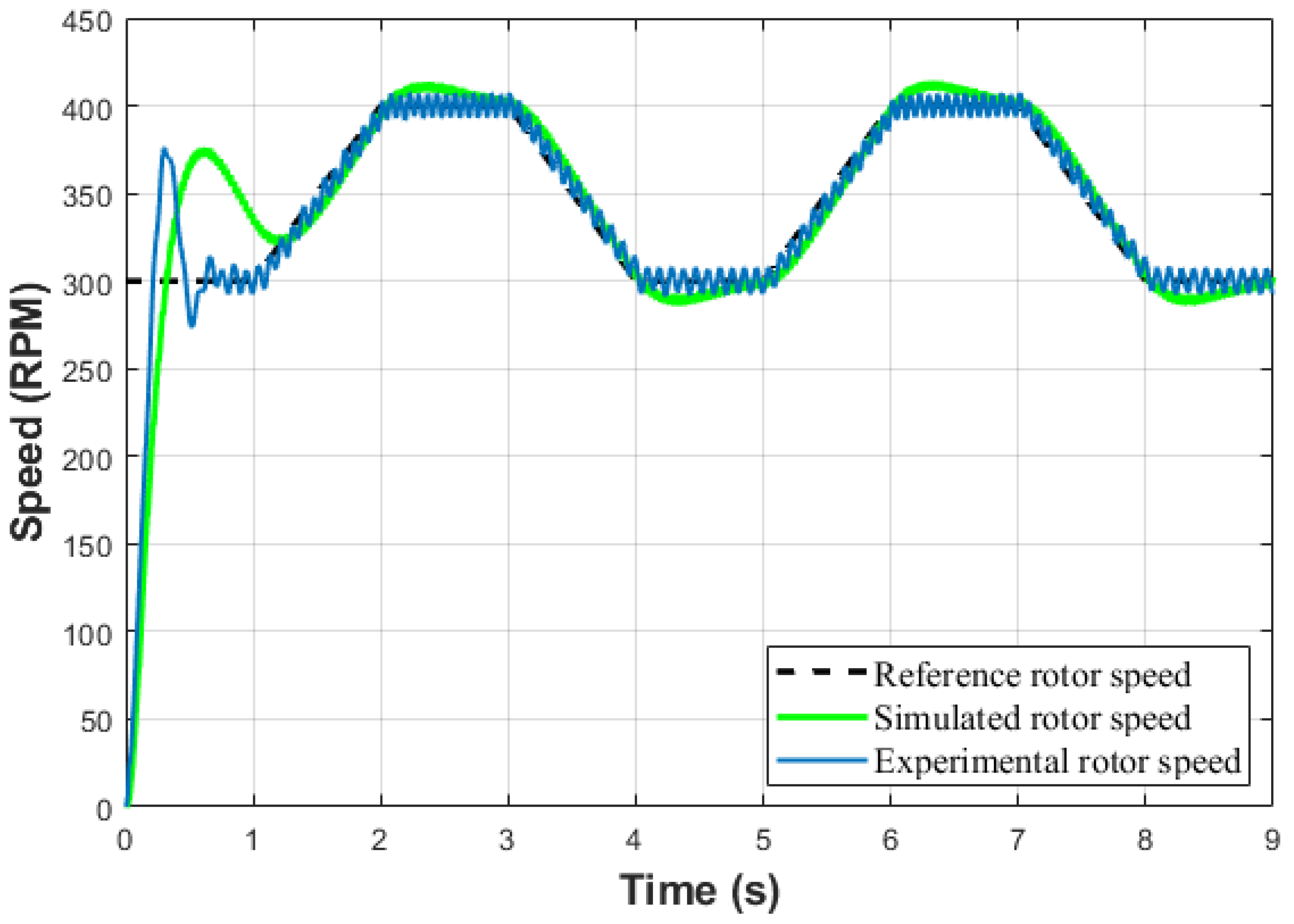
Figure 22 shows the machine speed behavior for a trapezoidal reference, with a lower reference of 300 RPM and higher than 400 RPM.
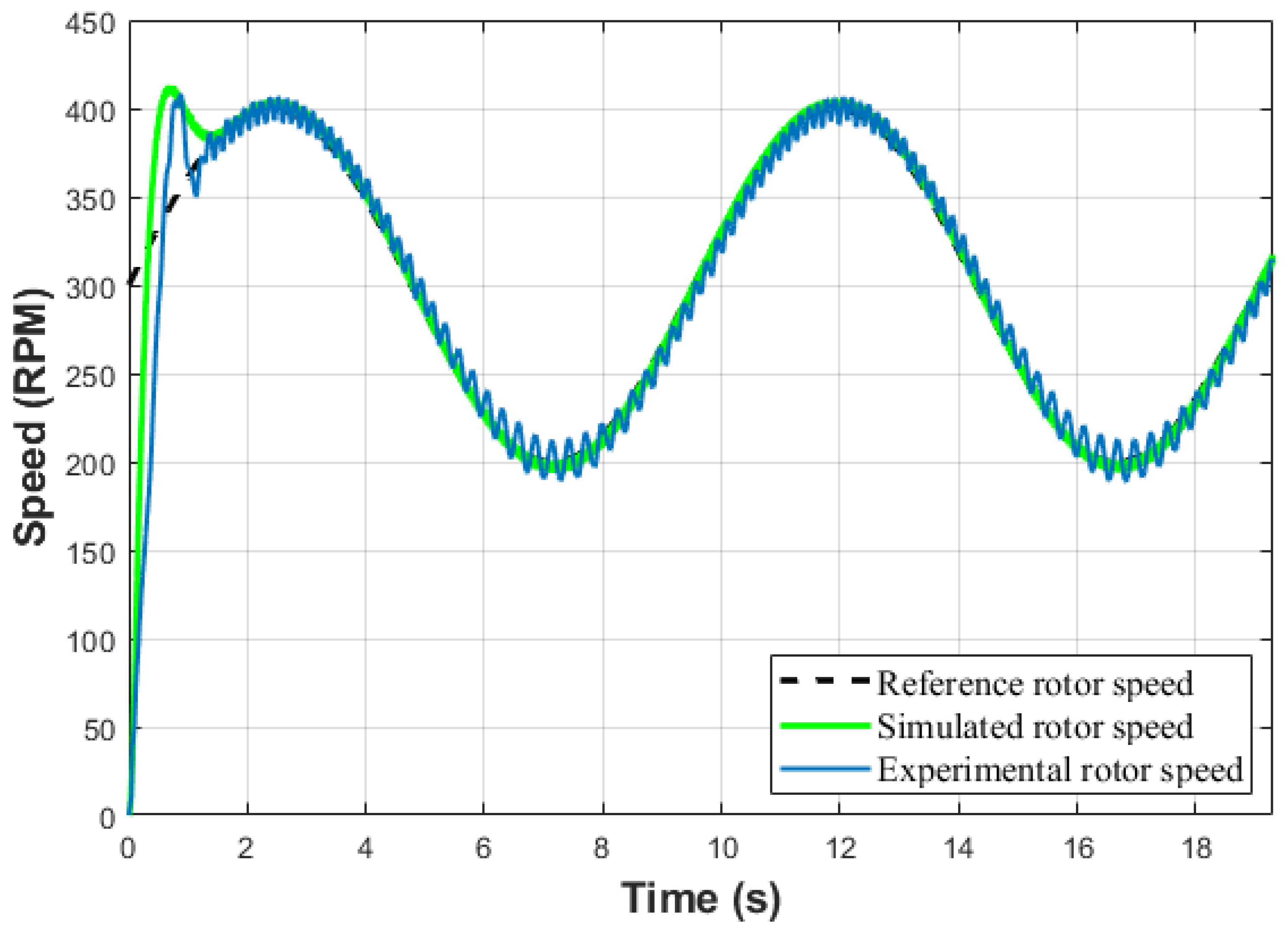
Figure 23 shows the behavior of the machine speed for a sine reference with a frequency of 0.1 Hz and amplitude of 200 RPM.
Analyzing the results for the different speed references, it is evident the correct functioning of the implemented speed control loop. It is important to highlight that due to the accuracy of the encoder available during the tests, the speed signal has low amplitude oscillations.
Table 8 presents the speed controller performance results for the three reference profiles.
The overshoot signal for the speed loop with different speed profiles shows little difference from the performance specifications. The closed loop of the speed controller has a zero that was disregarded for the calculation of the controller gains. In the experimental environment, this zero contributes to the divergence of the peak speed from the simulated speed signal.
Due to the accuracy of the electrical parameters obtained through routine tests to make up the machine model, the dynamic performance of the current and speed controllers both in simulation and in the experimental tests did not rigidly follow the design specifications. In addition, simplifications in the current loop were adopted concerning the coupling terms that influence the actual behavior of the machine. However, the divergences present in the compliance with the performance criteria did not compromise the operation of the indirect field-oriented control strategy. The results presented validate the correct operation of the hardware, control loops and the implemented strategy.
7. Conclusions
The built AC drive presented results within the expected range. Thus, the methodology adopted for the commissioning of the power circuit and acquisition system met the intended goals. The use of the FNA41560 power module made the construction of the converter more versatile and economically viable, and it can be used for different drive applications for small induction machines.
The results show that both current and speed controllers presented similar results to the results obtained during the simulation step. To solve the divergences in performance, settling time and overshoot, verified in the tests, it is proposed to implement feedforward compensation in the current control loop. Furthermore, as the machine used is of small size, it is difficult to obtain electrical parameters with good accuracy only with conventional blocked-rotor and no-load tests.
Vector control allows you to control the torque and flux of the machine independently. However, this technique is dependent on the angle of the rotor flux and the fidelity of the machine’s electrical and mechanical parameters. Thus, lines of research focus on approaches that use flux estimators or the use of controllers that are robust to parametric variations or adaptive or predictive type controllers.
SVPMW modulation proved to be an effective technique for driving the semiconductor switches of the IGBT bridge and relatively simplicity of implementation in the DSP. In addition, the use of this technique allows greater use of the voltage available on the DC link, reduced switching numbers and lower harmonic distortion in the machine line currents.
The developed test bench allows work focusing on other control strategies, activation of induction machines and PWM modulation techniques to be studied and validated.


 ,
, 


