Article

Multi-Frequency Weak Signal Decomposition and Reconstruction of Rolling Bearing Based on Adaptive Cascaded Stochastic Resonance

Key Laboratory of Advanced Manufacturing and Intelligent Technology, Harbin University of Science and Technology, Harbin 150080, China
*
Author to whom correspondence should be addressed.
Machines 2021, 9(11), 275; https://doi.org/10.3390/machines9110275
Submission received: 10 September 2021 / Revised: 30 October 2021 / Accepted: 3 November 2021 / Published: 8 November 2021
(This article belongs to the Section Machines Testing and Maintenance)

Abstract

:
In engineering practice, the bearing fault signal is composed of a series of complex multi-component signals containing multiple fault characteristics information. In the early stage of fault sprouting and evolution, the fault features are easily disturbed by noise and irrelevant signals, eliminating the fault signals in the strong background noise. To overcome the influence of noise on the signal, this study proposes multi-frequency weak signal decomposition and reconstruction of rolling bearing based on adaptive cascaded stochastic resonance. First, the original signal is passed through the Hilbert transform to obtain the envelope signal. The envelope signal is high-pass filtered to eliminate the interference of low-frequency components on the response of the stochastic resonance system. Secondly, cascaded stochastic resonance system parameters are adaptively optimized by the quantum particle swarm algorithm (QPSO). The high-pass filtered signal input to the adaptive cascaded stochastic resonance system (ACSRS) can further enhance the weak fault characteristics, allowing the gradual transfer of high-frequency noise energy to the low-frequency fault characteristic components. Finally, the signal is decomposed using the variational mode decomposition (VMD) method to jointly determine the location of the fault characteristic frequencies in the intrinsic mode functions (IMF) component by the energy loss coefficient and correlation coefficient to achieve the reconstruction of multi-frequency weak signals. Through simulation and experimental validation, the effectiveness and superiority of the method for multi-frequency weak signal detection in bearings are verified. The results show that the method not only achieves the adaptive optimization of the stochastic resonance system parameters gradually removing the high-frequency noise in the signal and improving the energy of the low-frequency signal but also reduces the number of decomposition layers of the VMD, enhances the fault characteristic information in the weak signal, and effectively identifies the early weak fault characteristics of rolling bearings.

1. Introduction

Rolling bearings, as the most important supporting parts of rotating machinery are called “industrial joints”; the application of rolling bearings covers almost all industrial fields. The operating condition of rolling bearings directly affects the efficiency, productivity, and life of the equipment. In rotating machinery failures, bearing failures account for about 30% of all failures [1,2,3]. In industrial sites, the complex working conditions of equipment bring great challenges for bearing fault diagnosis. There are more complex vibration disturbances between bearing components, and the collected vibration signals contain a large amount of interference noise, and the fault characteristics are difficult to be separated and easily drowned by the noise. Therefore, it is of great research value and practical significance to extract the weak signal characteristics of rolling bearings and grasp the operating status of bearings in time to realize early fault diagnosis. To solve this problem, many scholars have proposed different weak signal detection methods, such as Hilbert transform [4], wavelet transform (WT) [5], empirical mode decomposition (EMD) [6], and variational mode decomposition [7]. Morlet proposed the idea of “wavelet analysis” in 1984, and the wavelet transform can be used to analyze the signal to be measured in layers according to different scales, and to characterize the time-frequency properties of the signal locally [8,9]. The wavelet transform overcomes the limitation of the global nature of the traditional Fourier transform and solves the problem that the width of the window function of the Fourier transform is fixed. However, it is still limited by the difficulty of selecting the wavelet basis function and the difficulty of determining the scale range of wavelet decomposition. Empirical modal decomposition is an analysis method for adaptive processing of non-linear signals proposed by Dr. Huang et al. EMD decomposes the signal into several components of the basic model and one remaining item. The key to EMD is the ability to decompose a complex signal into a finite number of intrinsic mode functions (IMF), where the decomposed IMF components contain local features of the original signal at different time scales [10,11]. However, it still relies on the methods of finding extreme value points, envelope interpolation, and the selection of iterative termination criteria. Wu and Huang [12] proposed the ensemble empirical mode decomposition (EEMD) method. White noise is added to the original signal to automatically assign signals of different time scales to appropriate reference scales. Yaguo Lei et al. [13] used complete ensemble empirical mode decomposition with adaptive noise (CEEMDAN), which further reduces the modal effects by adding adaptive noise and has better convergence. Although both EEMD and CEEMDAN can effectively suppress the modal aliasing of EMD, they cannot effectively solve the endpoint effect problem. In 2014, Dragomiretskiy and Zosso proposed the variational mode decomposition (VMD) method. VMD uses an iterative search method to continuously update the center frequency and bandwidth of each BIMF component to obtain the optimal decomposition component and center frequency. Since VMD is influenced by the quadratic penalty factor and Lagrangian operator, the quadratic penalty factor can have good convergence characteristics and strict enforcement of constraints in the presence of noise [14,15]. VMD has a great advantage over EMD in that it has improved robustness to noise and can separate two similar frequencies from its construction and decomposition mode. Cancan Yi et al. [16] proposed a fault feature extraction method based on a combination of VMD and particle swarm optimization algorithms. The optimal penalty function and the number of decompositions in particle swarm optimization VMD are used, the ratio of the maximum value of the mean and the variance of the number of interrelationships is defined as the fitness function, the maximum correlation kurtosis is used to select the optimal component, which can effectively identify the weak fault information of rolling bearings. Ming Zhang et al. [17] proposed a new method for rolling bearing fault diagnosis based on VMD. The effects of gravity and unbalanced forces were considered, and the dynamic response models of faults at different locations were established. The performance of extracting bearing defect features in the simulated signals of rolling bearings with VMD and EMD was compared. The method was able to successfully diagnose rolling bearing faults. Tingkai Gong et al. [18] proposed a method based on VMD and trend filtering, which uses trend filtering to simplify the spectrum of the original signal, and the criterion of kurtosis adaptively selects the regularization parameters of trend filtering, which can effectively identify the compound faults of rolling bearings. Chunguang Zhang et al. [19] proposed a fault diagnosis method based on optimal VMD and resonant demodulation techniques. Combining genetic algorithms and non-linear programming algorithms, a new parameter optimization algorithm is designed to adaptively optimize two parameters of VMD. According to the maximum principle, the two most sensitive IMF components are selected for the reconstruction of the vibration signal. The reconstructed vibration signal is decomposed to obtain the envelope spectrum using the resonance demodulation technique, and the fault frequency of rolling bearings of locomotives is effectively identified. Xiwen Qin et al. [20] proposed a fault identification method based on VMD and iterative random forest (IRF) classifier. Comparing the fault recognition effects of EMD and EEMD new number decomposition and the combination of three mainstream classifier methods, VMD-IRF can better identify rolling bearing faults. Tao Liang [21] proposed a multi-objective multi-island genetic algorithm (MIGA) to optimize the VMD parameters and applied it to the feature extraction of bearing faults. The envelope entropy and renyi entropy are used as the fitness function to obtain the optimal solution of the VMD parameter using the MIGA algorithm. The two IMF with the most fault information is selected for reconstruction using the improved kurtosis and Holder coefficients. This method can extract the bearing fault characteristics more accurately. All of the above methods are based on noise suppression or elimination of noise in the vibration signal to identify fault characteristics. However, the process of denoising damages the weak fault features submerged in the strong noise background and cannot retain the complete fault signal, and its weak signal detection performance is limited. Stochastic resonance is the use of noise through a non-linear system to enhance the weak fault characteristics, which has certain advantages in weak signal detection.
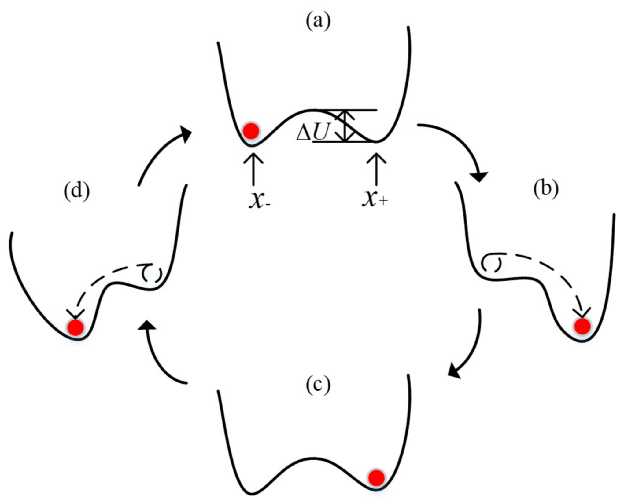
The concept of stochastic resonance (SR) was originally proposed by Benzi et al. [22] and used to explain the ancient glaciers meteorological issues, has since been used to describe non-linear systems in which the presence of internal or external noise can increase the response of the system output. In rotating machinery fault detection, the main research has focused on the application of a single stochastic resonance-enhanced single fault signal in weak feature extraction [23,24]. However, when the signal-to-noise ratio of the vibration signal is low, the detection effect of a single SR is difficult to identify multiple fault types of bearings. The actual bearing fault signal is composed of a series of complex multi-component signals containing multiple fault feature information, so multiple frequency components should be enhanced to distinguish different fault types in bearings. To solve the above problem, it is necessary to investigate the stochastic resonance enhancement technique of cascaded stochastic resonance [25]. Cascaded stochastic resonance is a single series-connected bistable system that achieves noise reuse through multiple filtering processes, further weakening high-frequency vibrations to make the output waveform smoother and the useful signal characteristics more obvious. Therefore, cascaded stochastic resonance is more advantageous than individual stochastic resonance in processing weak signals. Peiming Shi et al. [26] proposed an empirical mode decomposition method based on the denoising of cascaded multi-stable stochastic resonance systems. Using the cascaded multi-stable stochastic resonance system (CMSRS) as a denoising preprocessor, the energy is gradually transferred from high to low frequencies, and the denoised signal is decomposed using empirical mode decomposition. The method can gradually remove high-frequency noise, reduce the number of decomposition layers, improve low-frequency signal energy, and effectively identify bearing fault characteristic signals. Whether a single stochastic resonance method or a stochastic resonance enhancement method is used to extract useful characteristics in vibration signals, there is a common problem of how to select the appropriate system parameters to generate stochastic resonance. For this reason, adaptive stochastic resonance algorithms have been developed in the last decade [27,28]. Siqi Gong et al. [29] proposed a new method for weak signal detection based on wavelet transform and parameter optimization for bistable stochastic resonance. The wavelet coefficients are adjusted according to the variance of each detail and approximation coefficient and the frequency band in which the signal is located using the wavelet coefficients. The parameters of the stable stochastic resonance model are selected by the a priori information of the signal, and then the model parameters are adjusted according to the calculated local signal-to-noise ratio. This method can effectively detect weak signal characteristics hidden in strong noise. Z. H. Lai et al. [30] proposed an adaptive multi-parameter tuned stochastic resonance method for bistable systems based on particle swarm optimization algorithm, which generates optimal SR output by adaptively adjusting multiple parameters to achieve fault feature extraction and further fault diagnosis of rolling bearings. However, the cascaded bistable stochastic system involves multiple model parameters, the system parameters are difficult to adjust, the adjustment process is time-consuming, and engineers with insufficient experience may be unable to obtain the optimal SR output. Importantly, this makes the method of implementing stochastic resonance and fault diagnosis in practical engineering inefficient and unreliable. To solve these problems, various adaptive parameter tuning methods have been proposed and studied using multi-parameter optimization algorithms, such as particle swarm optimization [31] and genetic algorithms [32], which can implement stochastic resonance online in an efficient and highly reliable manner. To further improve the detection performance of the adaptive stochastic resonance method and extend its application in fault diagnosis, it is necessary to consider multiple parameters and propose the corresponding adaptive multi-parameter tuning cascaded stochastic resonance method.
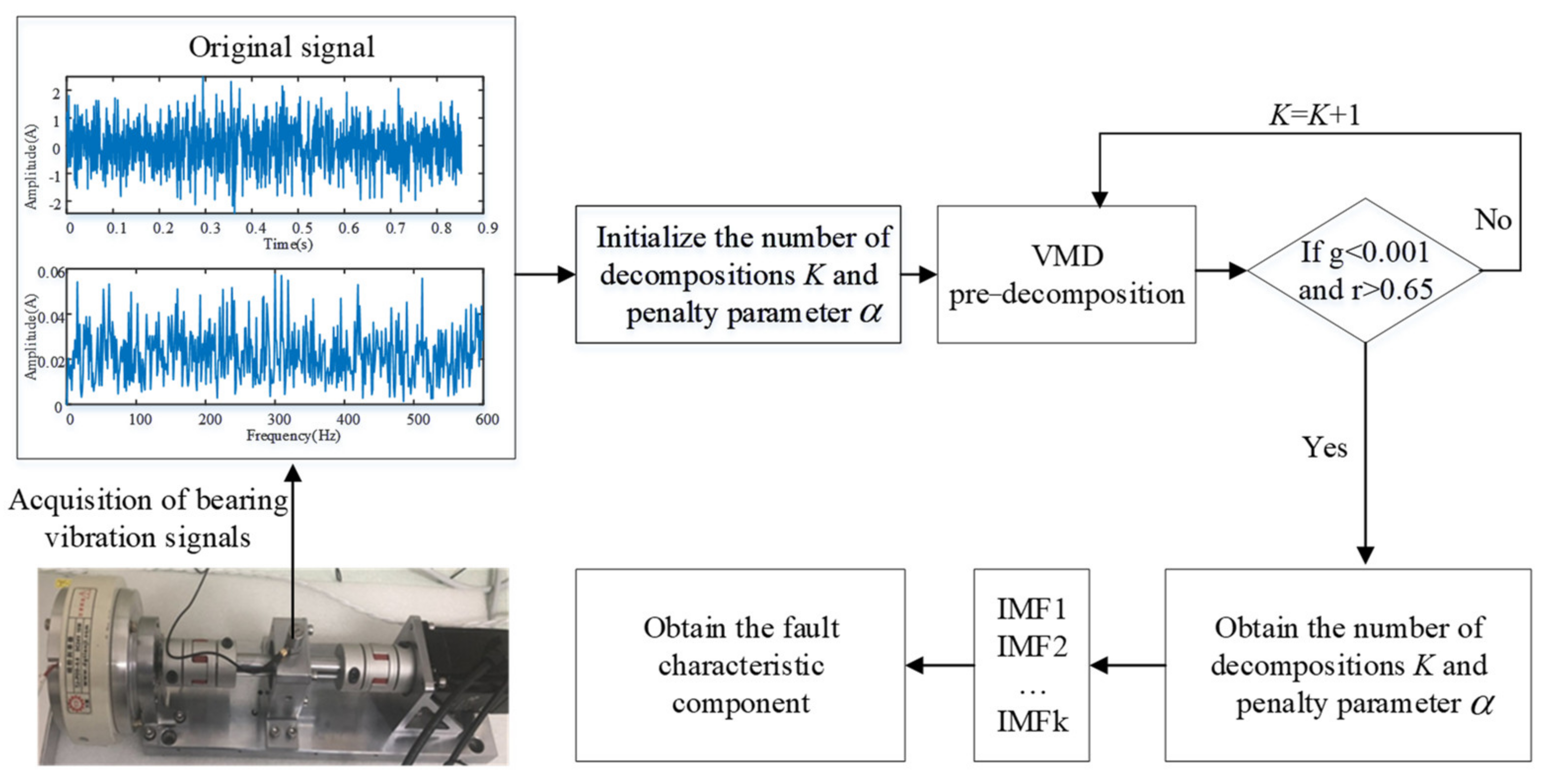
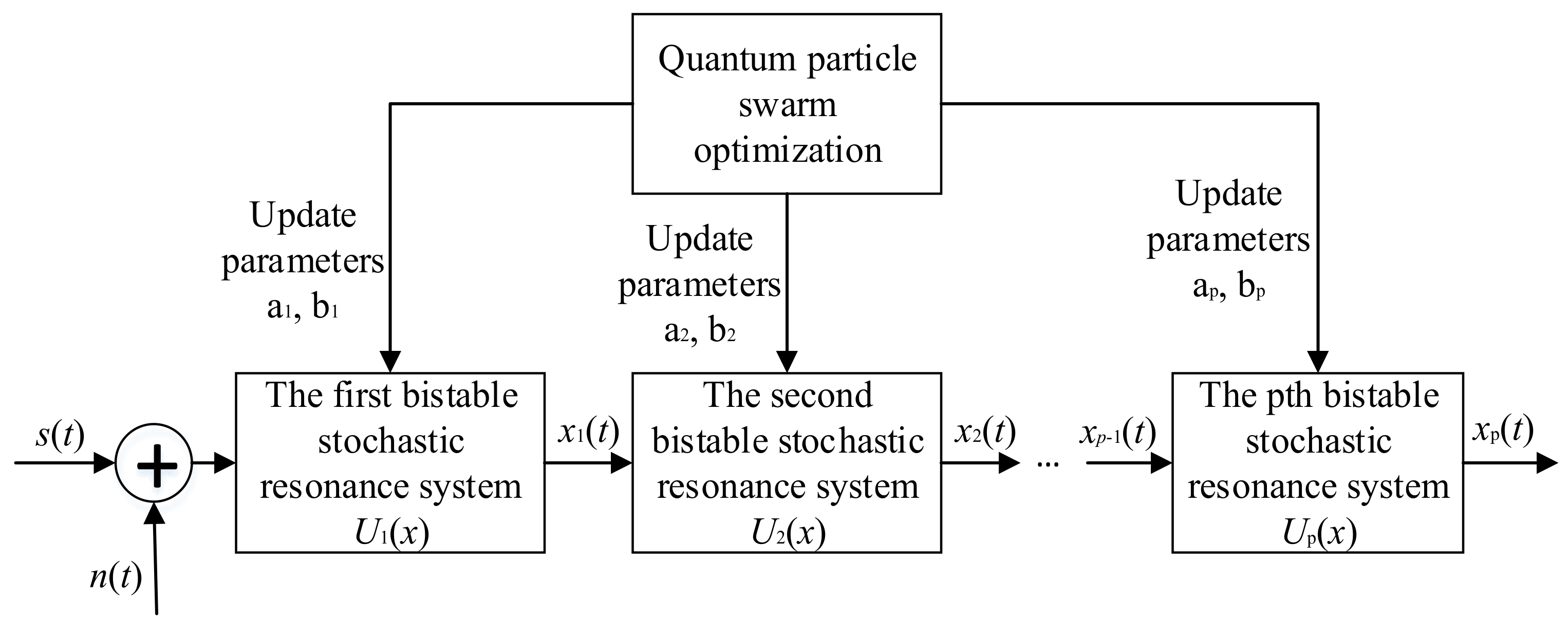
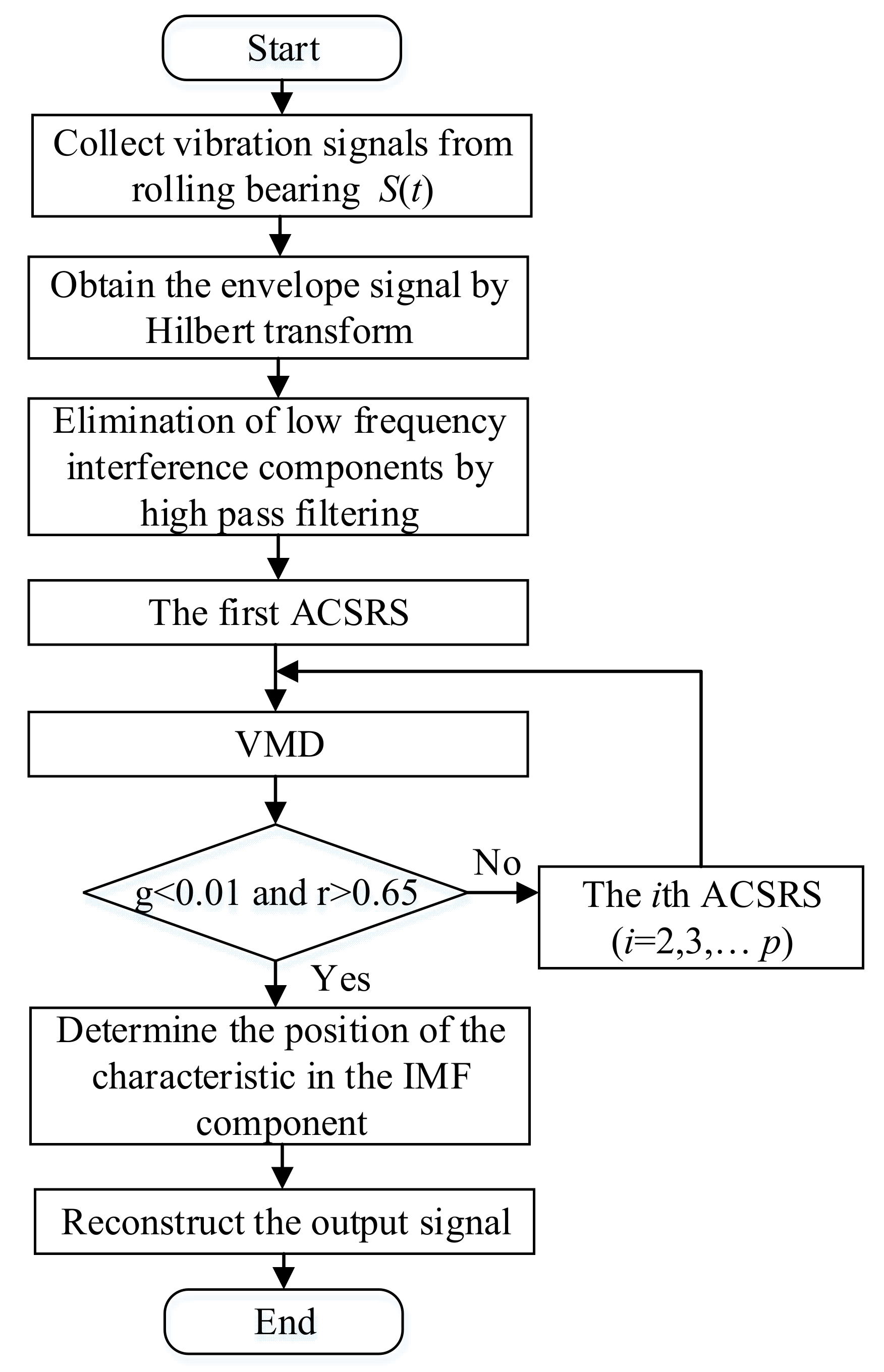
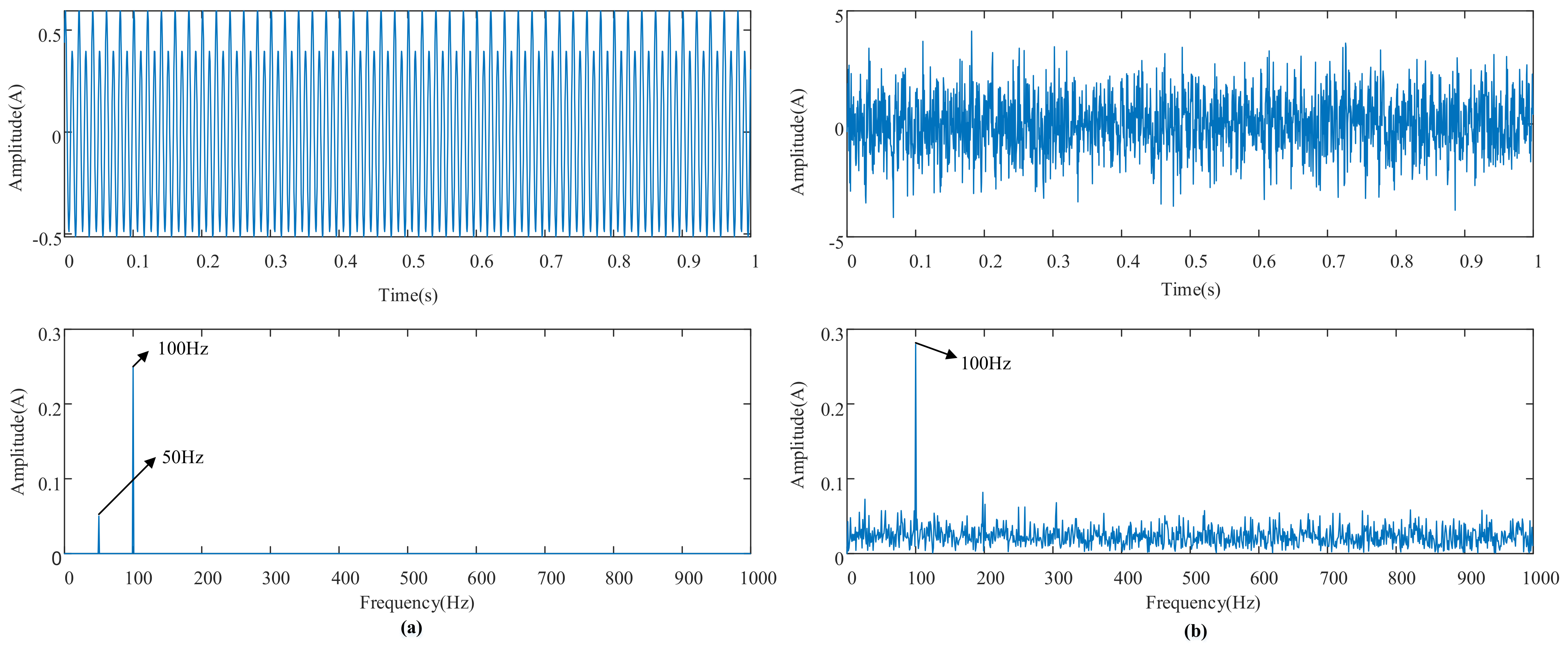
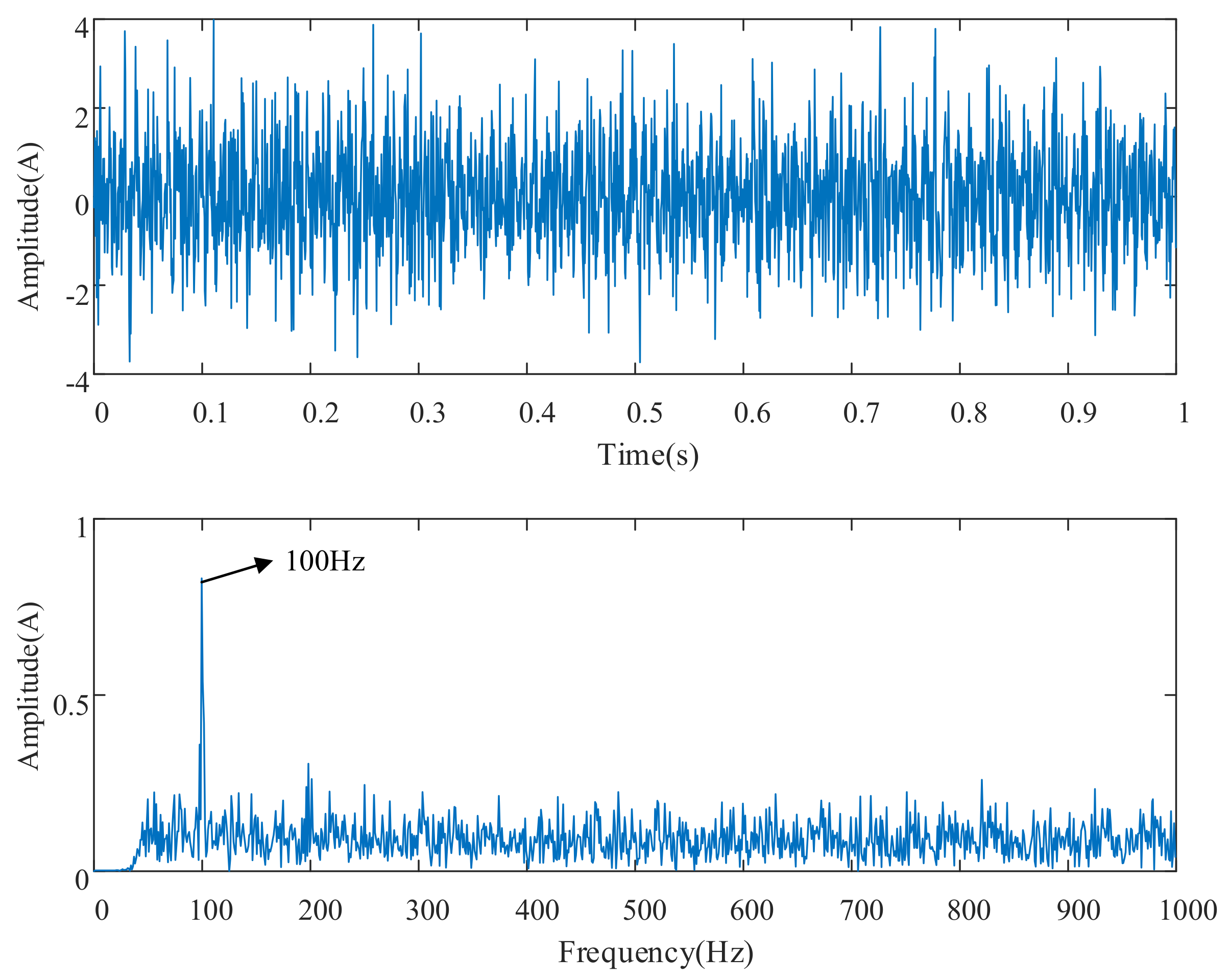
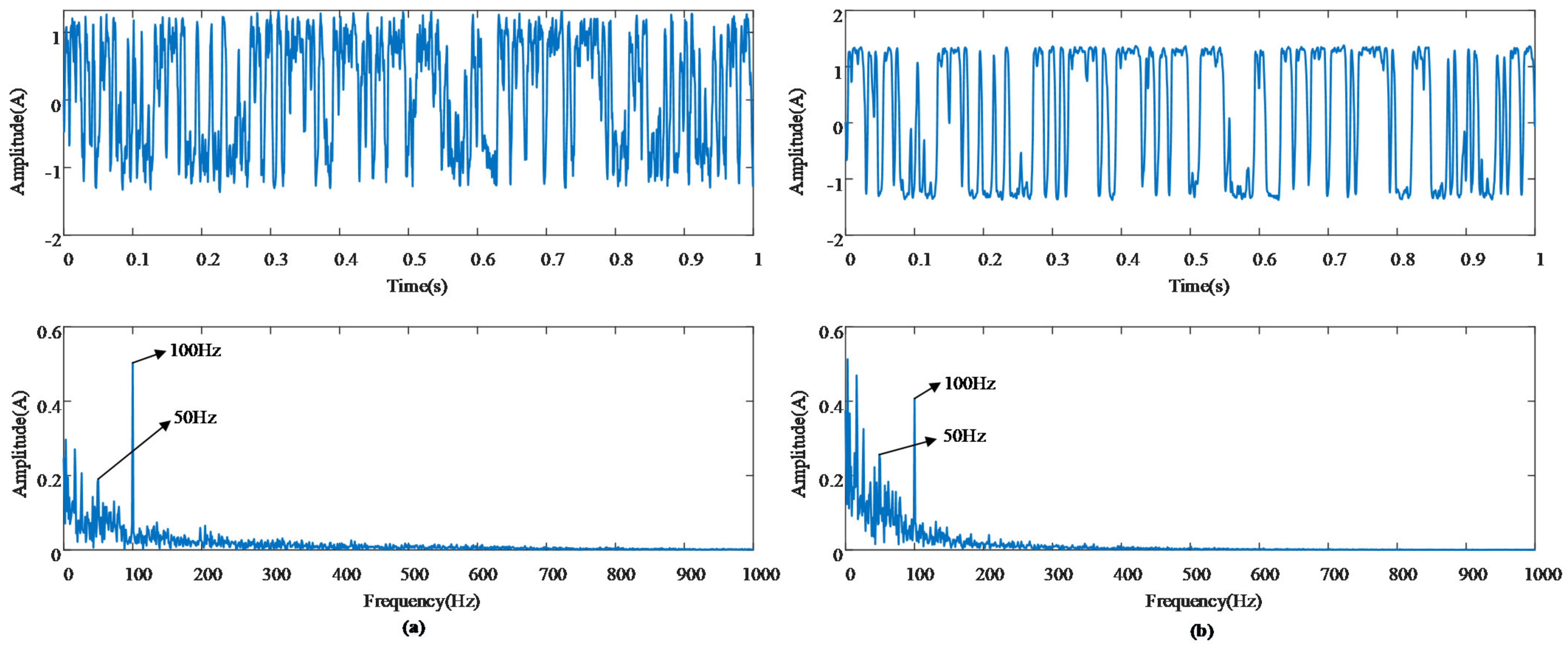
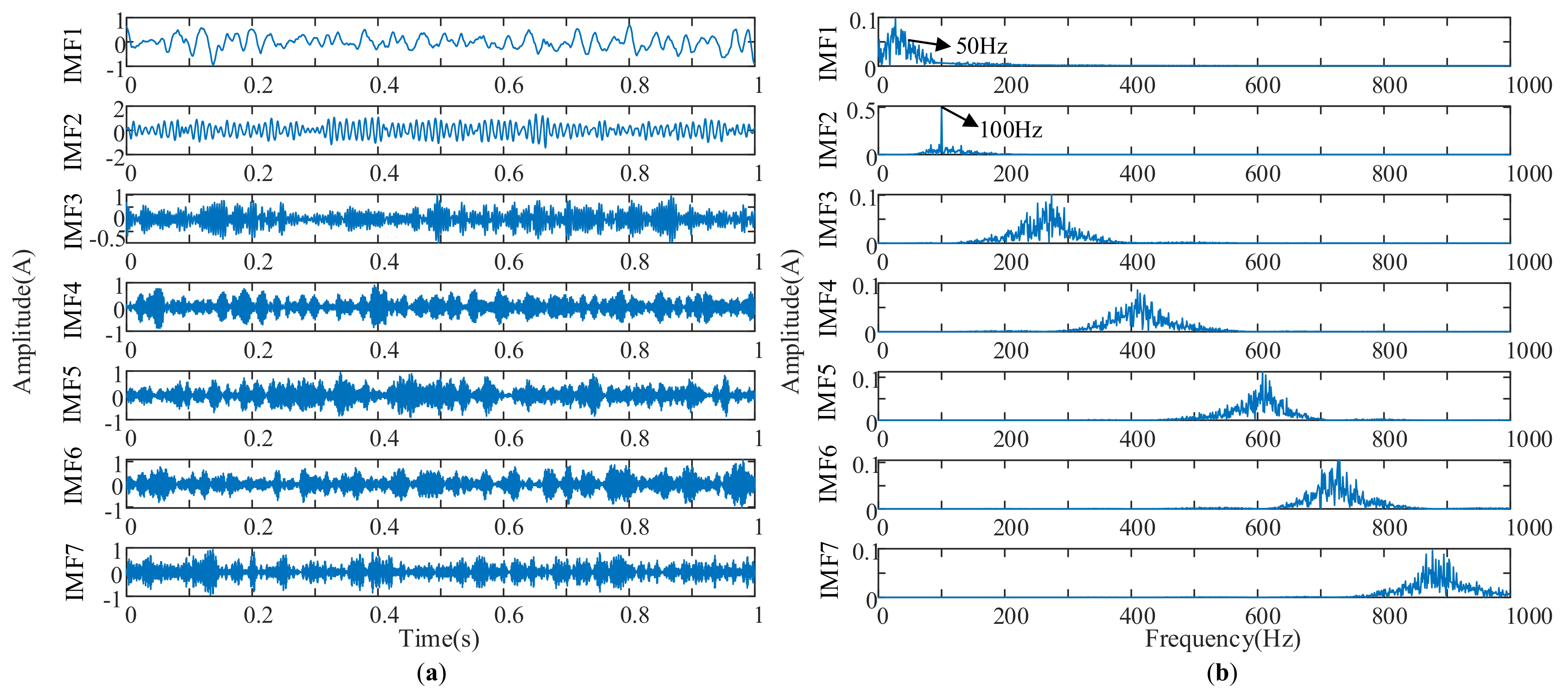
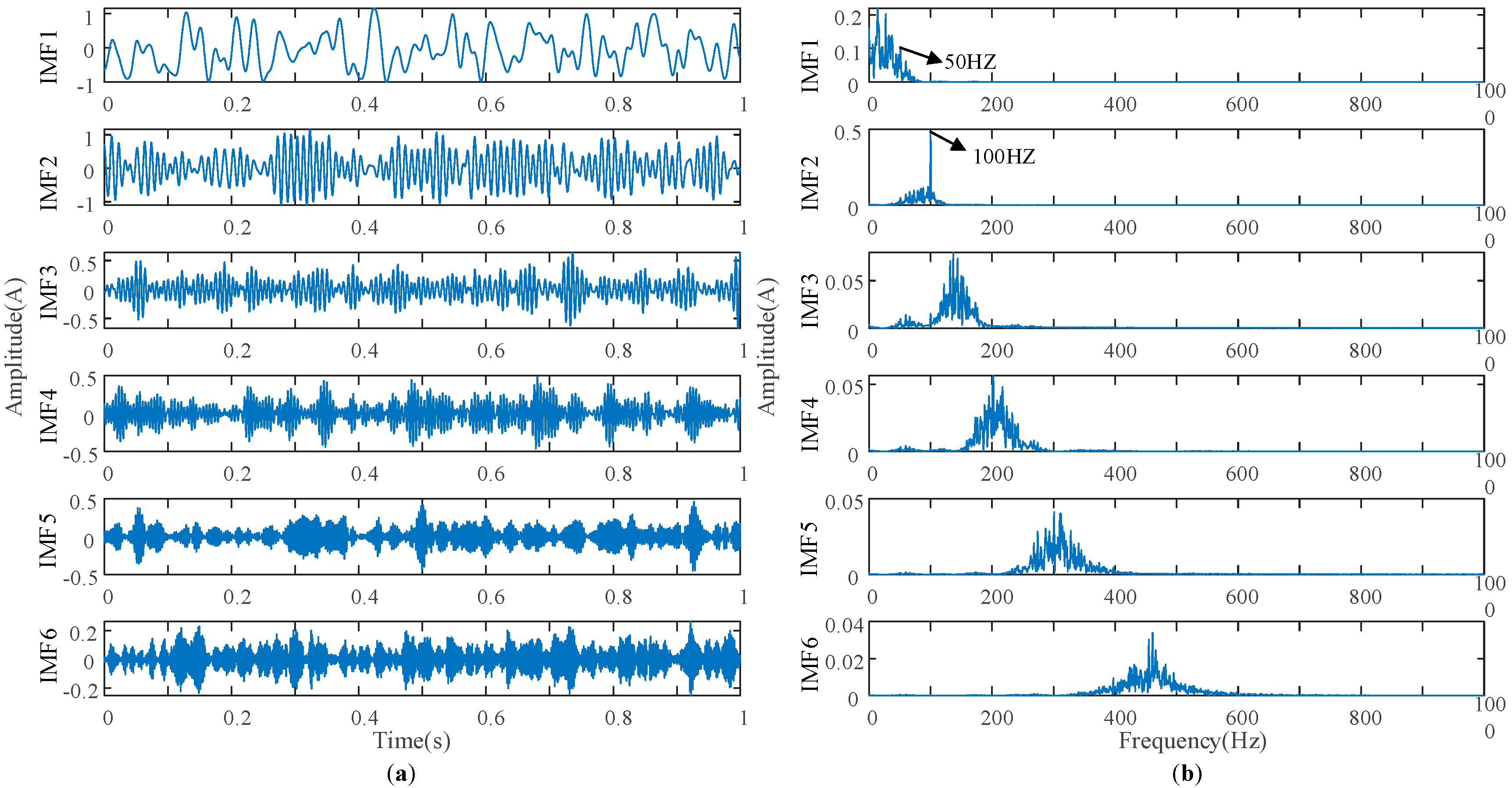
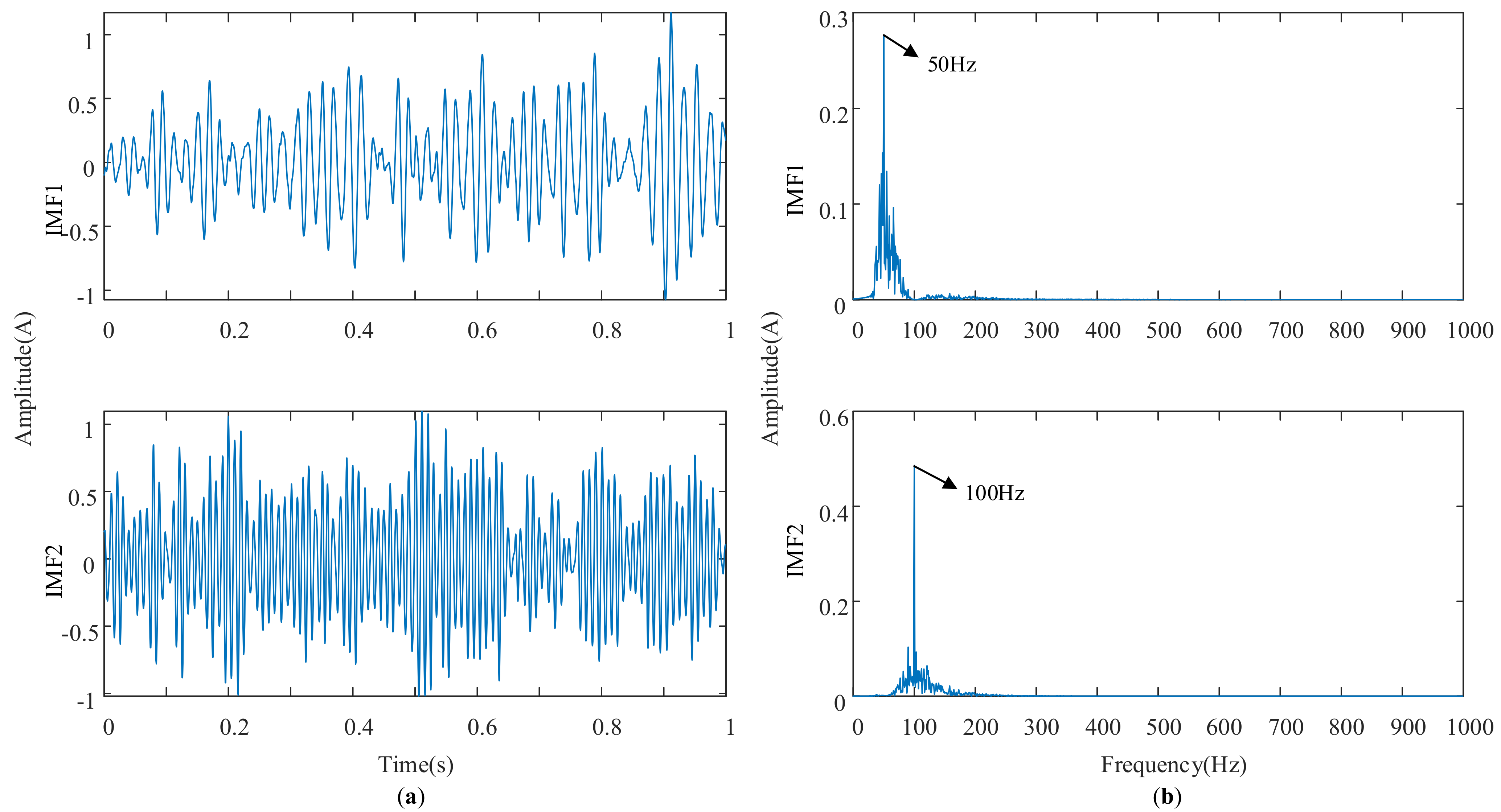
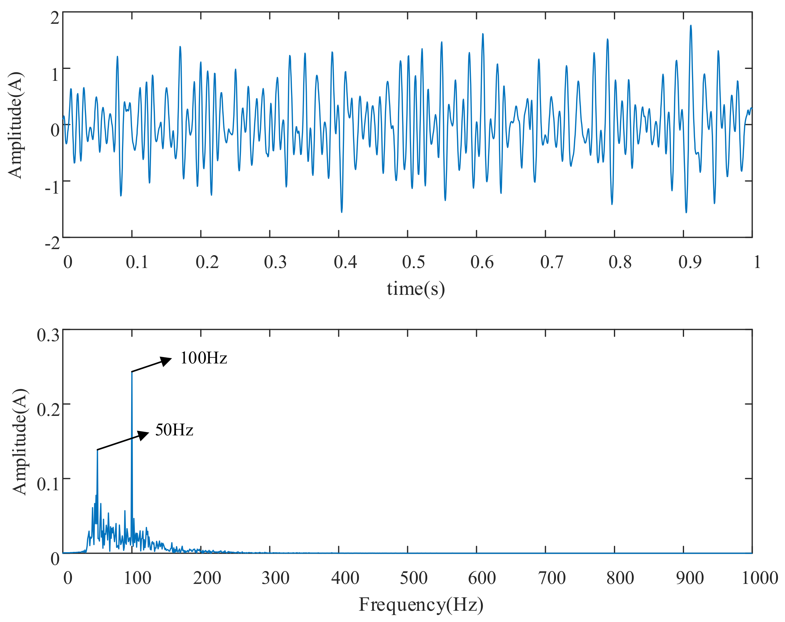
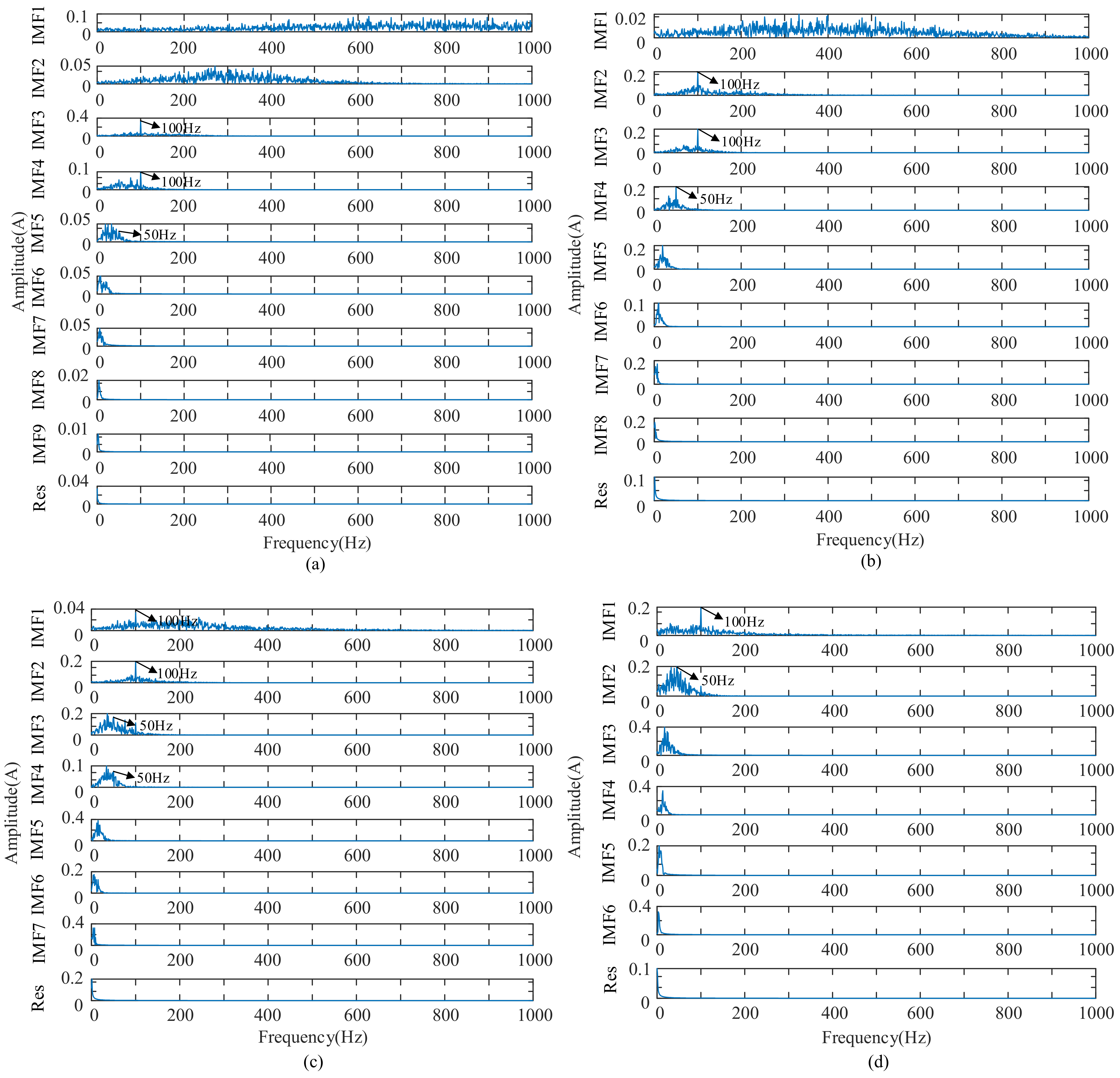
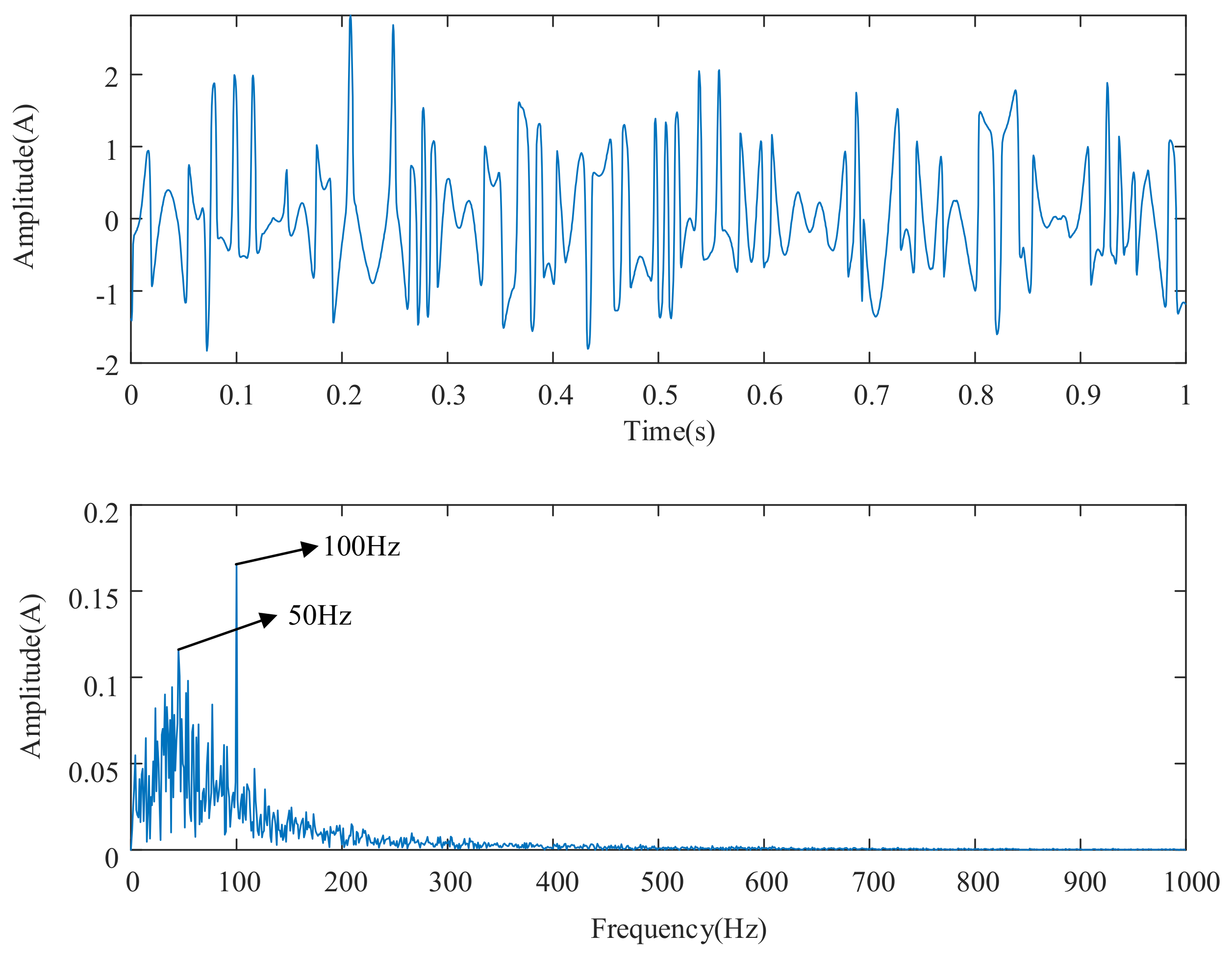
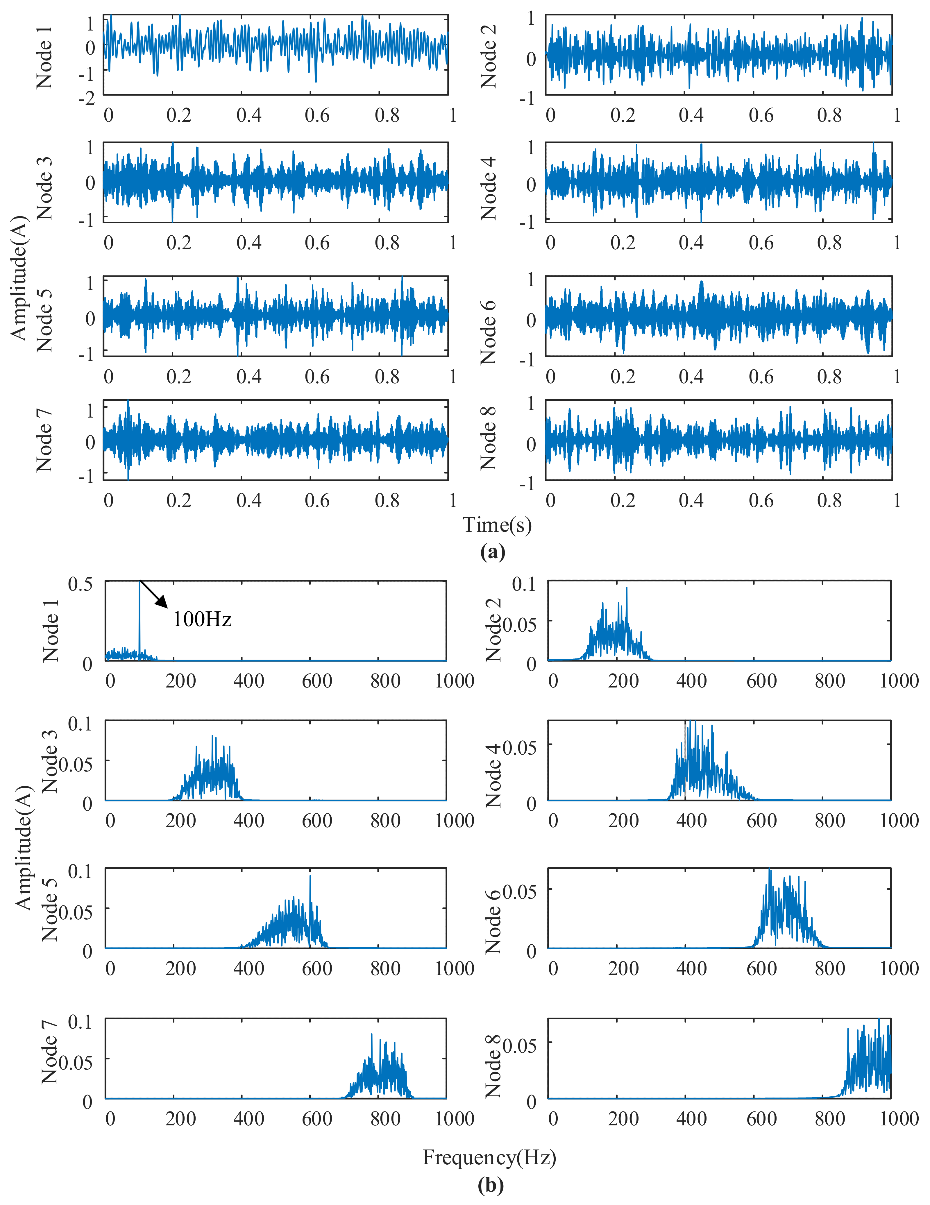
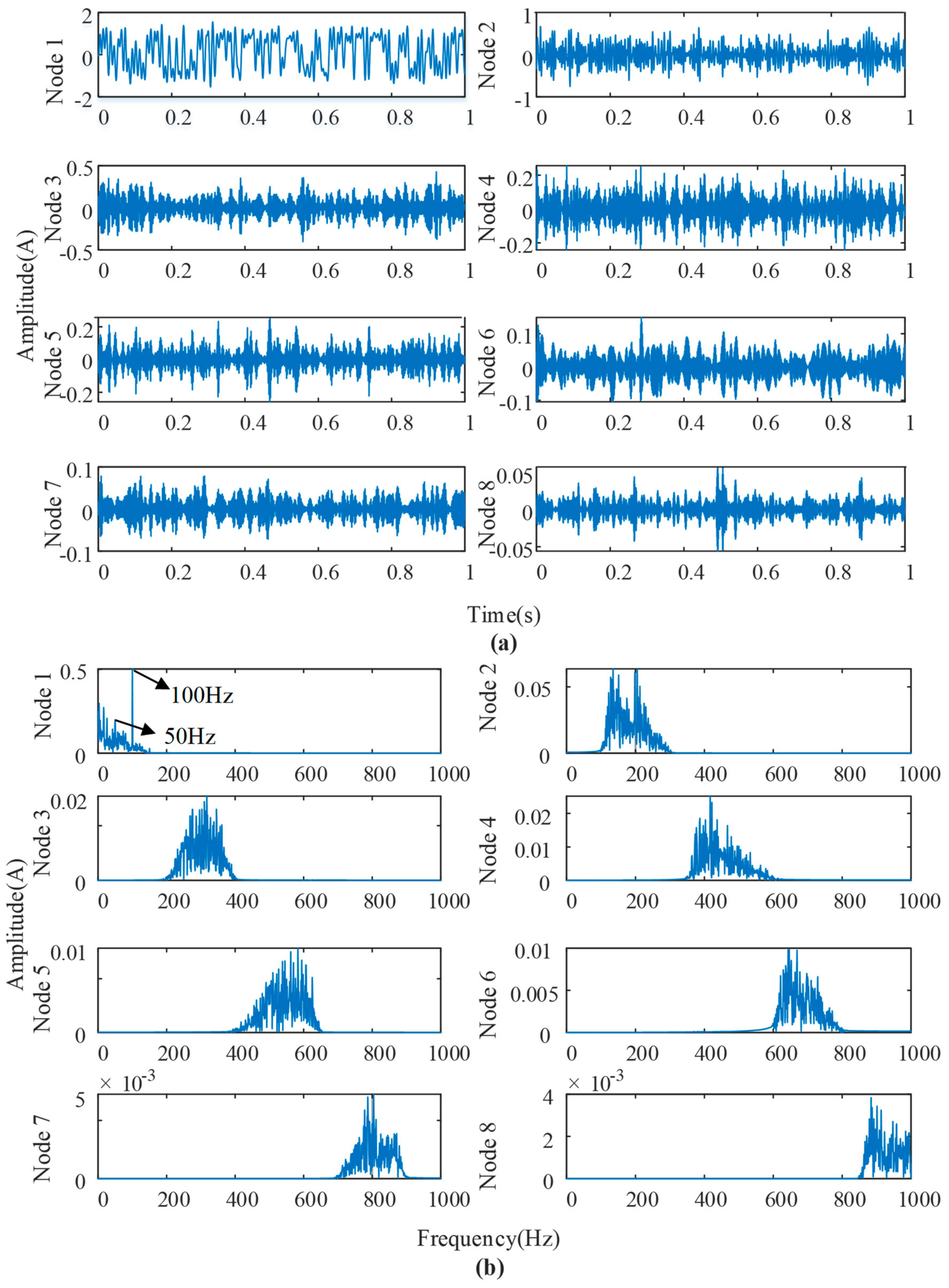
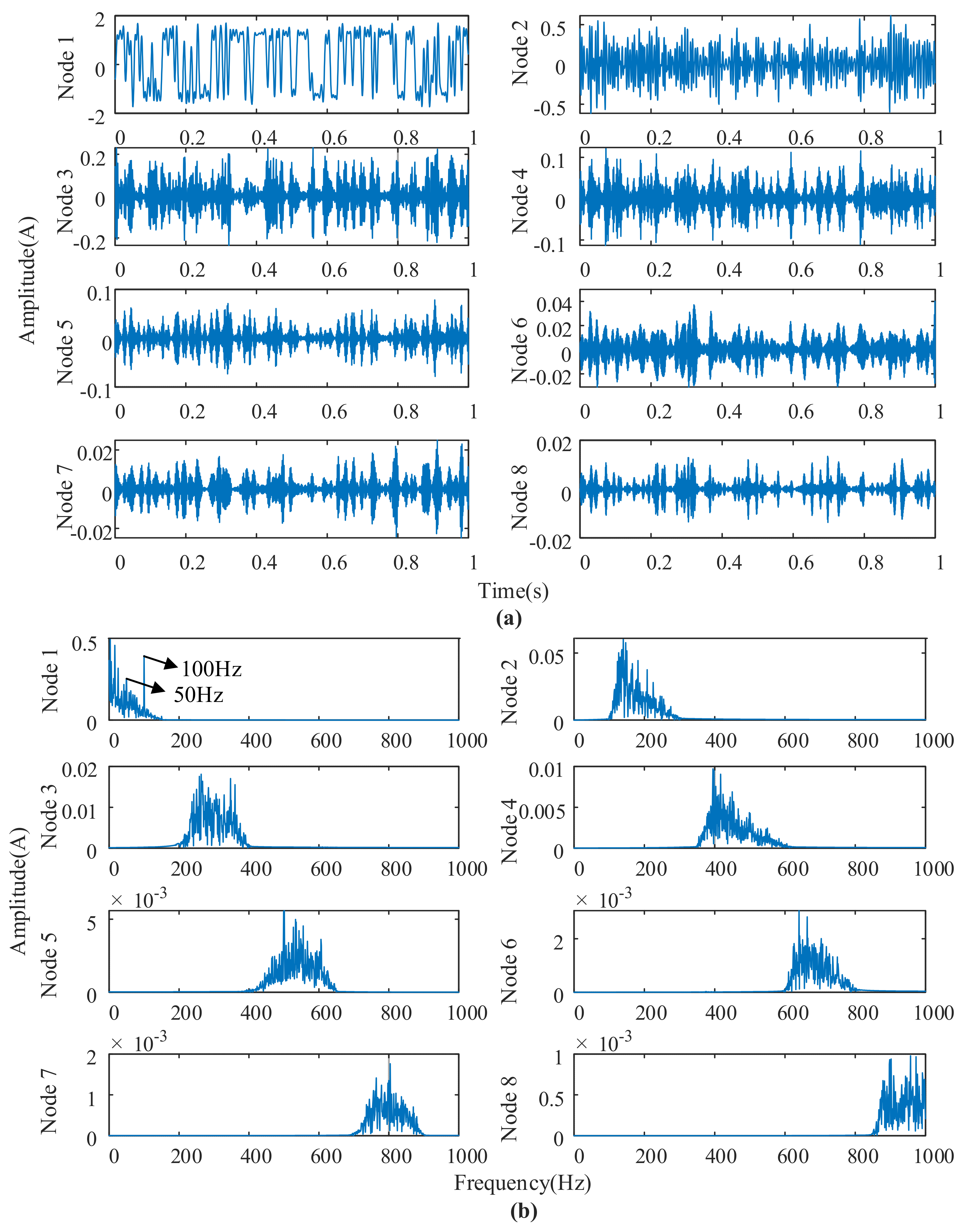
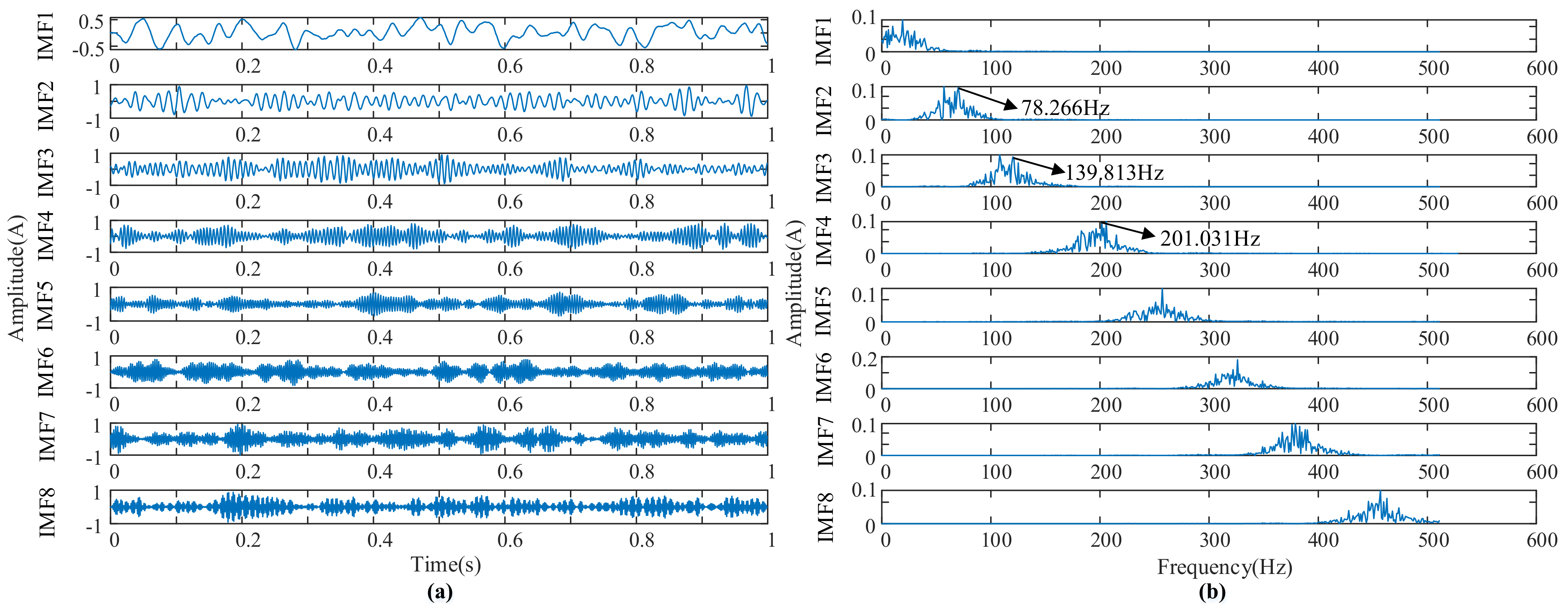
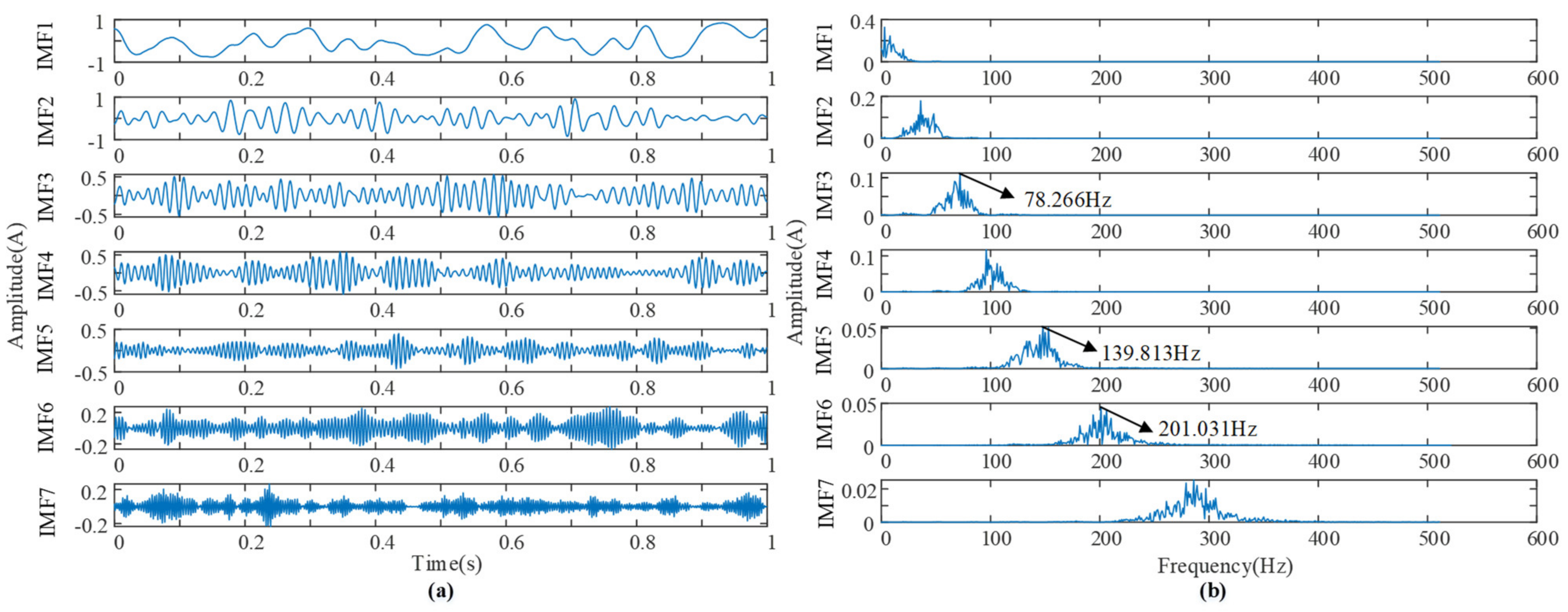
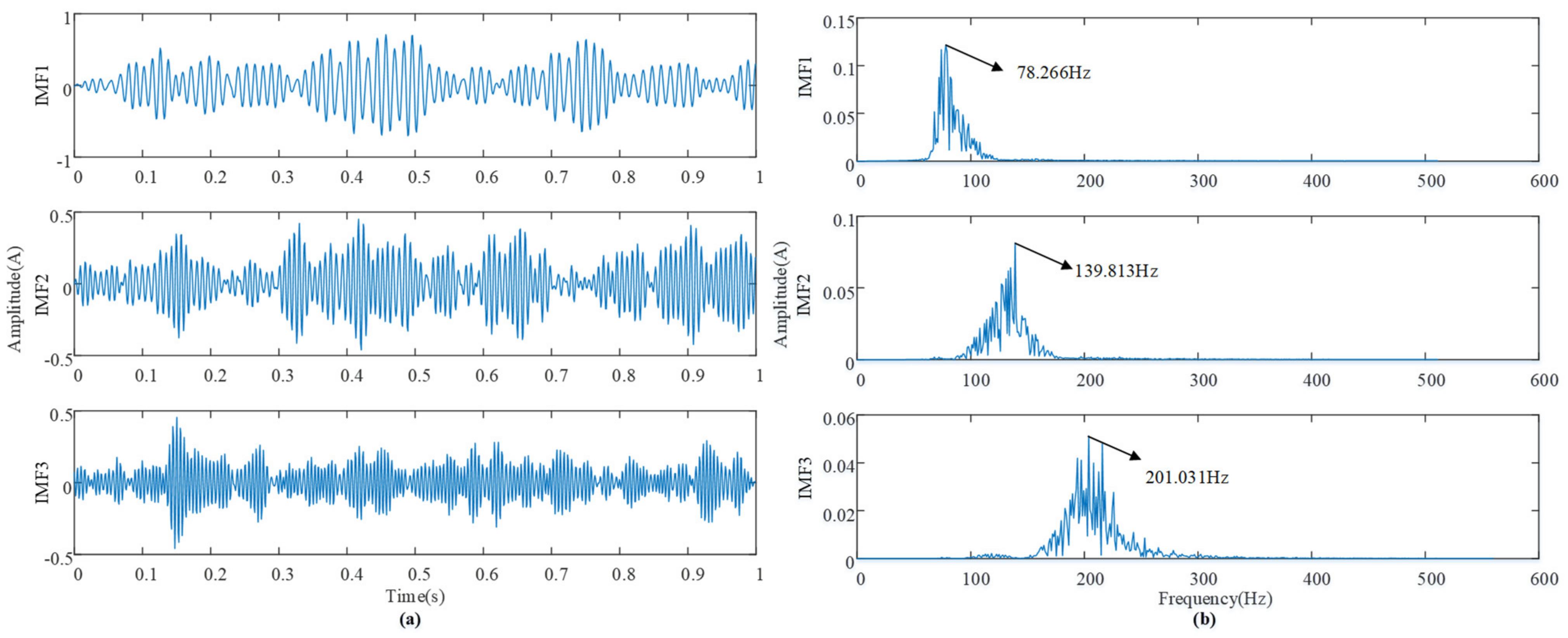
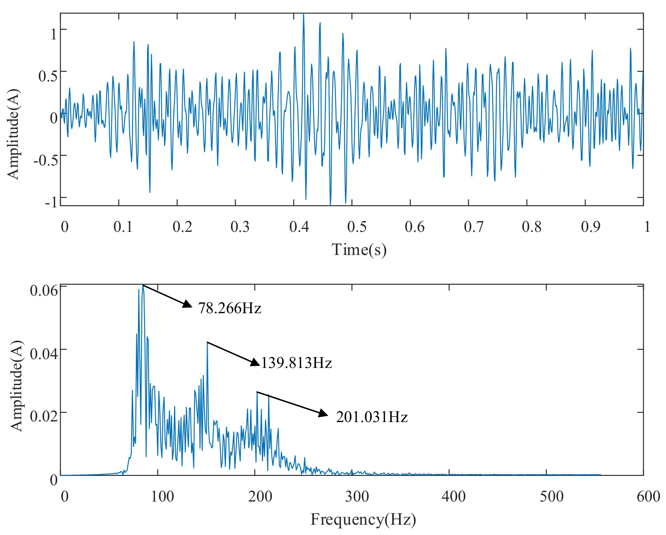
In summary, to achieve the detection of rolling bearing weak signals under strong background noise, combining the respective advantages of noise reduction and signal enhancement methods, this paper proposes an adaptive cascaded stochastic resonance method for decomposition and reconstruction of rolling bearing multi-frequency weak signals. Firstly, the original vibration signal is subjected to Hilbert transform to obtain the envelope signal, the envelope signal is high-pass filtered to eliminate the interference of low-frequency components on the response of the stochastic resonance system, the high-pass filtered signal is input to the ACSRS for signal enhancement, and the quantum particle swarm algorithm is used for adaptive optimization of the parameters in the cascaded stochastic resonance. Secondly, the enhanced signal after adaptive cascaded stochastic resonance is decomposed using the variational mode decomposition, and the energy loss coefficient and correlation coefficient are used to jointly determine the position of the characteristic frequency in the IMF component. The method can reduce the number of VMD decomposition layers while adaptively seeking the optimization of the parameters of the stochastic resonance system, so that the energy of the high-frequency noise is transferred to the low-frequency fault characteristic component, thus enhancing the fault characteristic information in the weak signal. Finally, the enhanced multi-frequency weak signal is reconstructed, which provides some reference ideas and methods for rolling bearing weak signal detection.
The rest of this paper is organized as follows: Section 2 introduces the variational mode decomposition theory method. Section 3, the proposed multi-frequency weak signal reconstruction based on adaptive cascaded stochastic resonance. Section 4 focuses on the experiment of rolling bearing compound fault validation of the proposed method. Finally, the conclusions are given in Section 5.

2. Variational Mode Decomposition Theory

VMD is a non-recursive adaptive signal decomposition method proposed by Dragomiretskiy et al. By solving the constrained variational problem, the arbitrarily complex multicomponent signal is adaptively decomposed into a series of IMF components based on the center frequency and finite bandwidth. In the solution process, the center frequency and bandwidth of each IMF component are continuously updated with the iterative process. Assuming that each “mode” is a finite bandwidth with a central frequency, the central frequency and bandwidth are continuously updated during the VMD decomposition process, and, finally, decomposed adaptively into K modal functions with the smallest sum of bandwidths u k t and the sum of K modal functions is the input signal S t . The objective of estimating the frequency bandwidth of the modal function by:
Hibert transformations are performed on each modal function u k t to obtain the analytic signal for each modal function, as follows:
δ t + j π t × u k t
Using the correction exponent e j w k t , the spectrum of each modal function is modulated to the respective fundamental frequency band, as follows:
δ t + j π t ×   u k t ×   e j ω k t
The squared L 2 parametrization of the gradient of the demodulated signal in Equation (2) is calculated to estimate the bandwidth of each modal function, corresponding to the constrained variational problem as follows:
m i n u k , ω k k = 1 K t δ t + j π t ×   u k t ×   e j ω k t 2 2 s . t . k = 1 K u k t   = S t
where u k denotes the individual variational modal components found, u k   =   u 1 , u K ; ω k denotes the central frequency corresponding to each component, ω k   =   ω 1 , ω K ; K represents the number of variational modal components, t denotes time, t is the partial derivative of the function for time t, δ t represents the unit pulse function, ω is the cyclic frequency, and S t is the input signal.
To transform the constrained variational problem into an unconstrained one, a quadratic penalty factor α is introduced to ensure the accuracy of signal reconstruction and convergence under noise conditions, a Lagrange multiplier operator L   is introduced to ensure the stringency of the constraints. The extended Lagrangian expression with the introduction of two parameters is:
L u k , ω k , λ = α k = 1 K t δ t + j π t ×   u k t ×   e j ω k t 2 2 + S t   k = 1 K u k t 2 2 + λ t , S t   k = 1 K u k t
where α represents the quadratic penalty factor; λ (t) denotes the Lagrangian multiplier.
The multiplicative operator alternating direction method is used to solve the extended Lagrangian expression, which is implemented as follows:
  • Initialize { u ^ k 1 } ,   { ω ^ k 1 } ,   λ ^ 1 ,   n ;
  • Execute the loop n = n + 1 ;
  • For all ω 0 , update u k and ω k ;
u ^ k n + 1 ω S ^ ω     i k u ^ i ω + λ ^ ω 2 1 + 2 α ω     ω k 2
ω k n + 1 0 ω u ^ k ω 2 d ω 0 u ^ k ω 2 d ω
λ ^ n + 1 ω λ ^ n ω + τ S ^ ω     k = 1 K u ^ k n + 1 ω
4.
Stop the iteration if the following convergence conditions are met, otherwise return to step 2.
k = 1 K ( || u ^ k n + 1     u ^ k n || 2 2 / || u ^ k n || 2 2 ) < ε
Ending the iteration, the IMF component with the minimum sum of K bandwidths is obtained.
Due to the complexity and diversity of the measured signal, the difficulty and key of the VMD algorithm are how to choose the appropriate decomposition number K and penalty parameter value α . When using VMD, it is necessary to choose the preset decomposition number K and penalty parameter α . The smaller the penalty parameter α in the VMD algorithm, the larger the bandwidth of each IMF component obtained by decomposition. The larger the value of the decomposition number K , the more likely it is to cause information loss. Before parameter optimization, the fitness function needs to be determined. k is chosen in such a way that no new central frequency maxima or minima appear, thus ensuring that the VMD decomposition does not miss higher or lower central frequencies. Therefore, the IMF component energy growth factor can be used as the fitness function. The energy growth factor g   is defined as the ratio of the energy difference between the current decomposition component and the previous decomposition component to the energy of the original signal.
G   = u k t u k 1 t 2 2 s t 2 2
where u k is the energy of the current decomposition component, u k 1 is the energy of the previous decomposition component, S t is the original signal. In this paper, the energy growth factor is used to determine the index of the number of modes, and the energy growth factor threshold g is set to 0.01 [33]. The maximum decomposition modulus K is set to 10 and the maximum penalty parameter α is set to 6000. Thus, by finding the minimum value of the energy growth factor, the number of decomposition modes and the penalty parameter can be determined adaptively, and the parameter optimization process of VMD is intuitively described as solving the minimization problem of the fitness function. In this paper, the correlation degree between the IMF component and the original signal is determined by the correlation coefficient r , which is calculated as follows:
r u k , S = C o v u k , S σ u k σ S
where C o v u k , S is the covariance of u k and S , σ u k , and σ S are the variances of u k and S , respectively. The value of r usually ranges between 0 , 1 , and the correlation degree can be empirically classified as follows: when r     0.8 , it is considered highly correlated when 0.5     r < 0.8 , it is considered significantly correlated when 0.3     r < 0.5 , it is considered as low correlation, and when r < 0.3 , it means that the correlation between two variables is extremely weak and is considered uncorrelated [34]. Therefore, the IMF components with a correlation greater than 0.65 are screened out, and the IMF components with significant correlation and high correlation with the original signal are screened out. The specific signal decomposition process of VMD is shown in Figure 1.
The original vibration signal of the bearing is obtained from the accelerometer of the rotating machinery failure experiment bench. The number of decomposition layers K and penalty parameter α are set before the VMD decomposition, and then the VMD pre-decomposition is performed. The decomposed IMF components are judged, if the energy growth factor threshold g is less than 0.001 and the correlation value r is greater than 0.65, the current number of decomposed layers K and the penalty factor α are output, and the current IMF is obtained. If it does not meet the requirement of increasing the number of K decomposition, then K = K + 1 , return to execute VMD pre decomposition until the condition requirements are met. The fault characteristic component of the rolling bearing vibration signal can be identified by VMD, but due to the influence of strong noise interference, the fault characteristic amplitude is low and the interference frequency amplitude is high, so it is difficult to identify the fault characteristic accurately. Therefore, it is necessary to transfer the high-frequency noise energy to the low-frequency signal through adaptive cascaded stochastic resonance, to strengthen the characteristic amplitude of weak multi-frequency signal and make it easier to identify its fault characteristics.

3. Multi-Frequency Weak Signal Reconstruction Based on Adaptive Cascaded Stochastic Resonance

3.1. Adaptive Cascaded Stochastic Resonance Model

SR can be described as a non-linear phenomenon, a Brownian particle is bistable by the weak periodic force and the stochastic force of the potential, and between the two, the particle can bounce off the potential well after the frequency of the weak periodic force with the assistance of the appropriate stochastic force.
This process can be represented by the stochastic differential equation as follows:
dx t d t = U x   +   S t   +   N t
where x is the particle trajectory, d t is the differentiation of the time, the low-frequency simple harmonic signal S 0 t = A 0 cos 2 π f 0 t + u 0   is the periodic signal with the frequency   f 0 much less than 1. S 0 t is the low-frequency weak signal to be detected,   u 0 are initial phase angles of low-frequency signal, N ( t ) is the zero-mean additive Gaussian white noise, the autocorrelation function satisfies N t , N 0 = 2 D δ t , where D is the noise intensity, U x   is the SR potential function. There are various types of SR potential functions, here only the classical bistable symmetric potential is considered as follows:
U x = 1 2 a 0 x 2 + 1 4 b 0 x 4
where a 0   and   b 0 are potential parameters with positive real numbers, which are usually set within 0 , 2 empirically. Figure 1 shows a schematic diagram of the Brownian particle jumping between bistable potential wells. The potential depth is calculated as Δ U   = a 0 2 / 4 b 0 . Assuming that the initial phase is   φ = 0 , the red dot indicates the initial position of the particle at the left-hand potential well, as shown in Figure 2a. At t = T / 4 , the potential is tilted under the excitation of the periodic signal S t , while the particle can jump from the left to the right potential well under the excitation of a suitable noise N t , as shown in Figure 2b. At   t = T / 2 , the potential well is re-equilibrated to S T / 2 = 0 , as shown in Figure 2c. At   t = 3 T / 4 , the potential is re-tilted by S t   and the particle can jump from the right to the left potential well, as shown in Figure 2d. Thus, under the combined excitation effect of   S t and the appropriate noise   N t , the particle oscillates between the two potential traps. Based on the particle trajectory x(t), the weak signal drowned in the noise is enhanced in the SR domain. Under the excitation of appropriate noise, the second-order stochastic differential equation can be rewritten as:
d x t d t = a 0 x b 0 x 3 + S t   +   N t
Meanwhile, the SNR of the SR system can be expressed as [22]:
SNR   = 2 a 0 2 A 0 2 e Δ U / D 4 b 0 D 2 = 2 Δ U A 0 D 2 e Δ U / D
The signal-to-noise ratio is influenced by the potential, signal, and noise parameters. The signal-to-noise ratio increases as the noise intensity D increases. Unlike the conventional filtering curve, in which the signal-to-noise ratio decreases as the noise increases.
The stochastic resonance model excited by the multi-frequency signal S t   = A 1 sin 2 π f 1 t + φ 1   +   A 2 sin 2 π f 2 t   + φ 2 can be expressed as [35]:
d x t d t = a x b x 3   +   A 1 sin 2 π f 1 t + φ 1   +   A 2 sin 2 π f 2 t   + φ 2   +   2 D ξ t
where   a and   b are much greater than a 0 and b 0 ,   A 1 , A 2 are signal amplitudes, f 1 , f 2 are signal frequencies much greater than 1,   φ 1 , φ 2 are initial phase angles, ξ t is standard Gaussian white noise with mean 0 and variance 1.
To introduce the implementation mechanism of the general variable scale approach, alternative variables are introduced.
x t   = z τ , τ = m t
where m represents the scale factor. Substituting Equation (16) into (15) gives:
d z τ d τ = a m z b m z 3 + A 1 m sin 2 π f 1 m τ + φ 1   +   A 2 m sin 2 π f 2 m τ + φ 2   +   2 D m ξ τ
Introducing alternative variables as:
a m = a 1 , b m = b 1 , f 1 m = f g 1 , f 2 m = f g 2
Substituting Equation (18) into (17), we obtain:
d z τ d τ = a 1 z b 1 z 3 + A 1 m sin 2 π f g 1 τ + φ 1   +   A 2 m sin 2 π f g 2 τ + φ 2   +   2 D m   ξ τ
When m   is a large enough constant, a 1 ,   b 1 ,   f g 1 ,   f g 2 are smaller parameters and have the same meaning as a 0 ,   b 0 ,   f 0   parameters. From Equation (17), it is easily understood that the signal amplitude and noise intensity are reduced by   1 / m times, to make them equivalent in terms of dynamical properties, the signal amplitude and noise intensity are amplified by m times, which can be rewritten as:
d z τ d τ = a 1 z   b 1 z 3 + A 1 sin 2 π f g 1 τ + φ 1   +   A 2 sin 2 π f g 2 τ + φ 2   +   2 D ξ τ
Therefore, to satisfy the small parameter condition of classical stochastic resonance theory, the large-parameter stochastic resonance model of the high-frequency signal in Equation (15) can be rewritten as
d x t d t = a x   a x 3 + m A 1 sin 2 π f 1 t + φ 1   +   m A 2 sin 2 π f 2 t + φ 2   +   2 D m ξ t
where, a ,   b ,   m A 1 ,   m A 2 ,   and   f 1 , f 2   are large parameters. Equation (21) is the ordinary re-scaling stochastic resonance model, which can detect weak signals with arbitrarily large frequencies. The ordinary re-scaling stochastic resonance model can match different noisy input signals with optimal potentials to improve the output signal-to-noise ratio. Compared with the normalized re-scaling stochastic resonance method, the ordinary re-scaling stochastic resonance method has obvious superiority in improving the signal-to-noise ratio. Particularly for the target signal with completely unknown signal amplitude and frequency, the ordinary re-scaling stochastic resonance method can further improve the ability to enhance and detect weak signals.
The stochastic resonance method has a unique signal processing mechanism for weak signal detection, which enhances weak features while reducing noise by transferring high-frequency energy from the signal to be measured to low-frequency to achieve weak feature extraction in a noisy background. However, the weak feature enhancement capability of single-stage stochastic resonance is limited, and the vibration signals generated by rotating mechanical parts, such as rolling bearings are usually multi-frequency signals, which are not effective for multi-frequency weak feature extraction in a strong noise background. Thus, the cascaded form of stochastic resonance system is used to induce the high-frequency energy in the signal to be measured to transfer to the low frequency continuously, so that the low-frequency weak feature energy is enhanced step by step, and the output signal-to-noise ratio of the system is further improved to finally realize the multi-frequency weak feature extraction in the strong noise background. Several single-stage segmented linear stochastic resonance systems are connected in series to form a cascaded bistable stochastic resonance system. The cascaded bistable stochastic resonance system can be expressed as:
d x 1 d t + d U l 1 x 1 d t = S t   +   N t d x i d t + d U l i x i d t = x i 1 t , i = 2 , 3 , P
where S t and N t denote the input signal and noise of the cascaded bistable stochastic resonance system, respectively, P denotes the number of stages of the cascaded bistable stochastic resonance system,   x i   denotes the output signal of the i -th level bistable stochastic resonance system U l i , which is also the input signal of the next level bistable stochastic resonance system.
In a cascaded bistable stochastic resonance system, several single-stage systems are organically connected through this series connection. For the single-stage system, the input signal is assisted by the noise after stochastic resonance, the high-frequency noise energy is transferred to the low frequency, and the low-frequency characteristic signal is enhanced. However, the cascaded stochastic resonance system involves multiple model parameters, and the system is unstable due to many parameters. In this paper, the quantum particle swarm optimization (QPSO) is used to optimize the structural parameters a and b in the stochastic resonance simultaneously, with the output signal-to-noise ratio of the system as the objective optimization function, aiming to maximize and optimize the output parameter values a and b . The optimal solution of the adaptive stochastic resonance method is obtained by adjusting the parameters. The cascaded stochastic resonance system has multiple levels of parameters, and each level of parameters can affect the final output effect. The adaptive cascaded bistable stochastic resonance model is shown in Figure 3. The steps of the QPSO algorithm are as follows.
  • Initialize the particle positions and set the number of populations, the maximum number of iterations, the dimensionality, and the search range of each dimension;
  • Let a i = a i + 1 ,   b i = b i + 1 , the adaptation value of the initial position of each particle is calculated, and the output signal-to-noise ratio corresponding to each particle is calculated according to the adaptation function, the corresponding signal-to-noise ratio value of the first generation of particles is taken as the local optimum of a single particle, and the maximum value of which is taken as the global optimum;
  • The particle position and velocity are updated according to the global optimum value to obtain the next generation of particles, and if the obtained local optimum solution or global optimum solution of a single particle is better than the previous generation of particles, the velocity and position of the corresponding single particle are updated, and the local and global optimum solutions are updated;
  • After reaching the maximum number of iterations, the optimal parameters a i ,   b i ,   a i + 1 ,   b i + 1 are obtained according to the positions of the final particles, and the values of   a i ,   b i are fixed, and the optimal solutions of   a i + 1 ,   b i + 1 are searched again in the range around a i ,   b i ;
  • The parameters a p ,   b p of the P -level cascaded bistable stochastic resonance system are calculated and the output signal is obtained.

3.2. Decomposition and Reconstruction of Multi-Frequency Weak Signals of Rolling Bearings

To achieve the detection of rolling bearing weak signals under strong background noise, this paper proposes a method based on adaptive cascaded stochastic resonance for multi-frequency weak decomposition and reconstruction of rolling bearings, which improves the quality and accuracy of VMD while increasing the computing efficiency. Therefore, the number of stages of the ACSRS needs to be chosen so that all the high-frequency noise energy of the enhanced signal VMD is transferred to the low-frequency modal components. The process of multi-frequency weak signal decomposition and reconstruction is shown in Figure 4. The specific framework of weak signal decomposition and reconstruction is as follows.
  • Hilbert transform of rolling bearing vibration signal to obtain the envelope signal;
  • High-pass filtering of the envelope signal eliminates the interference of low-frequency components to the response of the stochastic resonance system;
  • Inputting the high-pass filtered signal into the ACSRS for signal enhancement processing;
  • Adaptive optimization of the parameters in the cascaded stochastic resonance using quantum particle swarm optimization;
  • The VMD decomposition is performed on the output signal of the first ACSRS to determine the position of the characteristic frequency in the IMF component. The algorithm stops if all the high-frequency noise energy is transferred to the low-frequency modal component, g < 0.001, and the correlation r > 0.65;
  • If g > 0.001 or r < 0.65 then continue with the VMD decomposition of the enhanced signal from the next level of the ACSRS until the condition is satisfied;
  • Based on the extracted feature signal, the enhanced signal is reconstructed to achieve multi-frequency weak signal fault detection.

3.3. Simulation Experimental Verification

The simulated signals are composed of sine signals and the test signals are generated as follows:
S t   = 0.1 sin 2 π × 50 t + π 3 +   0.5 sin 2 π × 100 t + π 4   +   N t
The number of sampling points is 10,000, the sampling frequency is set to 2000 Hz. The noise simulation uses Gaussian white noise with noise intensity   D = 1.2 , and the simulated signal and its frequency spectrum are shown in Figure 5a. Figure 5b shows the time domain and frequency domain diagrams of the vibration simulated signals after adding noise. It can be observed that it is difficult to notice the periodic signal from the time domain waveform, and due to the large noise, only the frequency of 100 Hz can be seen from the frequency spectrum, and the frequency component of 50 Hz is submerged in the strong noise.
First, the rolling bearing simulated signal is passed through the Hilbert transform and then input to the high-pass filter, where the passband cutoff frequency and the stopband cutoff frequency of the high-pass filter are set to 45 Hz and 30 Hz, respectively. The time-frequency spectrum of the high-pass filtered signal is shown in Figure 6. The high-pass filtered signal is then fed into the ACSRS for processing. The time scale   m is taken as 1000 when the signal is pre-processed by an ordinary variable scale. The parameters in the ACSRS are optimized using QPSO, setting the maximum number of iterations T m a x = 200 , the population size H = 50 , and the optimization search intervals for   a 1 and b 1 are 0 ,   2 , respectively. The parameters of the first ACSRS optimized by QPSO are a = 1.0025 and b = 2 , the parameters of the second ACSRS are a = 0.888 and b = 1.4091. The time-frequency domain waveform of the ACSRS is shown in Figure 7. After the first ACSRS processing, the characteristic signal at 50 Hz in the input signal gradually appears, and the output waveform of the second ACSRS is smoother than that of the first ACSRS, and the cascaded stochastic resonance can obtain a higher signal-to-noise ratio. At the characteristic frequency of 50 Hz, the peak of the output spectrum of the cascaded stochastic resonance is much larger than the peak of the input spectrum, and the peak of the output spectrum of the second ACSRS is larger than that of the first ACSRS, and the weak feature enhancement of the cascaded stochastic resonance is stronger. By analyzing the output signal-to-noise ratio of the cascaded stochastic resonance, we can see that the signal-to-noise ratio of the simulated signal is 6.8642 dB, and the output signal-to-noise ratio of the first ACSRS is 7.9734 dB, which is 1.1616 times higher than that of the input signal. the output signal-to-noise ratio of the second ACSRS is 10.9773 dB, which is 1.3767 times higher than that of the first ACSRS. The weak feature enhancement capability of cascaded stochastic resonance is higher than that of single-stage stochastic resonance. However, the transfer of high-frequency signal energy to low-frequency signal significantly increases the energy of low-frequency signal, making the signal around the characteristic frequency 50 Hz increase more, affecting the effective identification of the characteristic frequency. Since the adaptive cascade stochastic resonance alone does not identify multi-frequency weak signals well, this paper proposes a method to decompose and reconstruct the original signal by combining adaptive cascade stochastic resonance with the VMD decomposition method. The energy-constrained variational mode decomposition is used to process the noise-reduced simulated signal, and the energy convergence factor g = 0.001 is set. The optimal number of decomposition layers k is determined based on the energy factor, and the energy convergence factor g is derived as shown in Table 1.
From Table 1, it can be seen that g 6 < g considers that the signal can be decomposed completely when the modal number is 7. Therefore, the VMD decomposition of the simulated signal is performed and the decomposed time-frequency domain is obtained as shown in Figure 8. It can be seen from the figure that the fault frequencies 50 Hz and 100 Hz appear in the first and second modal components, respectively, and the remaining components are multiples of the fault frequency, respectively, and the cascaded stochastic resonance signal enhancement is performed on the decomposed signal, as shown in Figure 9 and Figure 10.
Through the experiment, it can be found that after the original signal is decomposed by VMD, the correlation analysis finds that the components of the signal are distributed in each IMF component, and each IMF component is correlated with the original signal, as can be seen from Table 2. After the first ACSRS, the number of decomposition layers of the original signal by VMD decomposition is reduced to 6, and the correlation analysis shows that the correlation of IMF1 is 0.6156 and the correlation of IMF2 is 0.6914, and the energy of the high-frequency signal is transferred to the low-frequency component, which enhances the fault characteristics to be consistent with the frequency band where the fault characteristics are located in the simulated signal. Then, after the second ACSRS, the original signal is reduced to two layers by VMD decomposition signal decomposition, and the correlation analysis yields IMF1 correlation of 0.8052 and IMF2 correlation of 0.6503. The signal-to-noise ratio of the first ACSRS-VMD signal enhancement is 16.3357 dB, an increase of 2.0488 times compared to the first ACSRS. The signal-to-noise ratio of the second ACSRS-VMD signal enhancement is 20.5308 dB, an increase of 1.3878 times compared to the first ACSRS-VMD. The characteristic frequencies 50 Hz and 100 Hz are in the IMF1 component and IMF2 component, respectively, and then the original signal is reconstructed to obtain the reconstructed signal as shown in Figure 11, the fault rate can be observed from the figure where the high-frequency noise component is well filtered, and the high-frequency noise energy is transferred to the low-frequency component, which enhances the intensity of the fault signal and enables the detection of multi-frequency weak signals. To verify the effectiveness of the method in this paper, EMD decomposition and wavelet packet decomposition are used to verify the comparison experiment, respectively.
The EMD adaptive decomposition into 9th order IMF component and 1st order residual component Res is shown in Figure 12a. It can be seen from the figure that the components related to the fault frequency are mainly concentrated in the first 5th order IMF components, which shows that there is modal mixing in the signal and the fault characteristics are relatively weak and not easy to identify. The EMD result after the first ACSRS signal enhancement is shown in Figure 12b, the signal is decomposed into the 8th order IMF component and the 1st order residual component Res, the characteristic frequency is decomposed in the first 4th order IMF, there is still modal aliasing, the signal-to-noise ratio is 7.8294 dB compared to the input signal is improved by 1.1406 times. The EMD result after the second ACSRS signal enhancement is shown in Figure 12c; the signal is decomposed into the 7th order IMF component and the 1st order residual component Res. Compared with the EMD result after the first ACSRS, the number of decomposition orders is reduced by one, and the characteristic frequency is decomposed in the first 3 orders of IMF. The signal-to-noise ratio is 10.9843 dB, which is 1.4029 times higher than that of the first ACSRS. The EMD result after the third ACSRS signal enhancement is shown in Figure 12d, the signal is decomposed into six orders of IMF components and one order of residual Res. Compared with the EMD result after the second ACSRS, the decomposition order is reduced by one order, and the characteristic frequency is decomposed in the first two orders of IMF. The signal-to-noise ratio is 11.5992 dB, which is 1.0559 times higher than that of the second ACSRSR, and the reconstructed signal is shown in Figure 13.
The signal decomposed by wavelet packet is shown in Figure 14; the wavelet packet adopts the wavelet basis function db3; the number of decomposition layers is 3 [36], the characteristic frequency is concentrated in the 1-node frequency band of the third layer of the wavelet packet, and the wavelet packet decomposed signal after the first ACSRS shows that the 50 Hz frequency hidden in the noise background can be identified, as shown in Figure 15. The signal-to-noise ratio is 7.0930. The wavelet packet decomposition signal after the second ACSRS has an increased low-frequency characteristic spectrum peak compared with the wavelet decomposition signal after the first ACSRS, and the signal-to-noise ratio is 10.6739 dB, which is 1.5048 times higher than that of the first stage, as shown in Figure 16. The signal is reconstructed, and the first three wavelet packet node coefficients are selected for reconstruction, and the reconstructed signal is obtained as shown in Figure 17, from which the characteristic frequencies of 50 Hz and 100 Hz can be identified, but there are some interference components in the low-frequency part.

4. Experimental Validation and Analysis of Results

To verify the effectiveness of the proposed method in terms of bearing fault diagnosis under actual working conditions, a rotating machinery test bench was used to conduct bearing fault simulation tests, which mainly included: SGM7J-04AFC6S servo motor, rated speed 3000 RPM, YMC122A100 acceleration sensor, POD-0.6 Kg magnetic powder brake, rated torque 6 N∙m, and speed 2000 r/min. The 7204C/P5 bearing was used as the test object with a sampling frequency of 1024 Hz, and the specific parameters are shown in Table 3. Three bearing states were used for the test, and the bearing compound failure experiment was conducted using wire-cut machining to simulate the degree of bearing failure, which simulated the compound failure experimental data obtained from the inner race, outer race, and ball race of the bearing at defects depth of 0.5 cm. The specific structural components of the test bench are shown in Figure 18.
Figure 19a shows the composite fault vibration signal of a bearing with inner ring, outer ring, and roller faults. The rolling bearing vibration signal was subjected to Hilbert transform and then high-pass filtering, and the passband cutoff frequency and the stopband cutoff frequency of the high-pass filter are set to 70 Hz and 60 Hz, respectively, and the time-frequency spectrum of the high-pass filtered signal is shown in Figure 19b. The high-pass filtered signal is then fed into the ACSRS for processing. The two-parameter a = 1.207 and b = 2 for the first ACSRS optimized by quantum particle swarm, and the two-parameter a = 0.6865 and b = 2 for the second ACSRS. The output spectrum of the two-stage ACSRS is shown in Figure 19. The signal-to-noise ratio of the original signal is 3.6438 dB, and the signal-to-noise ratio of the first ACSRS is 7.8772 dB, which is an increase of 2.1618 times over the original signal. The signal-to-noise ratio of the second ACSRS is 9.0201 dB, which is an increase of 1.1451 times over the first ACSRS. The time-frequency domain signal after the first ACSRS enhancement is shown in Figure 20a. The high-frequency noise is partially transferred to the low-frequency region, enhancing the fault signature signal amplitude, but it is still difficult to identify its fault signature frequency. The time-frequency domain signal is shown in Figure 20b after being enhanced by the second ACSRS. The fault characteristic signal amplitude is further enhanced, and the fault frequency at the beginning of the ball race can be identified, while the rest of the fault frequencies are still difficult to identify. Therefore, VMD decomposition is used to decompose and reconstruct the signal, and the initial number of VMD decomposition layers is determined as eight layers by energy loss factor, as shown in Table 4. The decomposed time-frequency diagram is shown in Figure 21. The signal is decomposed into 8th order IMF components, and the fault features are decomposed in the 2nd, 3rd, and 4th order IMFs. The rolling element fault frequency is 78.266 Hz, the outer race fault is 139.813 Hz, and the inner race fault is 201.031 Hz. The error between actual fault frequency and theoretical fault frequency is less than 10%. The correlation analysis obtained an IMF1 correlation of 0.3627, IMF2 correlation of 0.3816, and IMF3 correlation of 0.3726.
The VMD results after the first ACSRS are shown in Figure 22, where the signal is decomposed into 7th order IMF components, and the fault features are decomposed in the 3rd, 5th, and 6th order IMFs. The correlation analysis obtained an IMF1 correlation of 0.6140, IMF2 correlation of 0.5033, and IMF3 correlation of 0.4680. Figure 23 shows the VMD result after the second ACSRS, the signal is decomposed into 3rd order IMF components, compared with the VMD result after the first ACSRS, the decomposition order is reduced by 4, and the correlation analysis obtained an IMF1 correlation of 0.8273, IMF2 correlation of 0.6975, and IMF3 correlation of 0.6980, as shown in Table 5. The fault features are decomposed in the 3rd order IMF, and the feature frequencies are obvious and easy to identify. The signal-to-noise ratio of the first ACSRS−VMD signal is 12.7407 dB, which is 1.6174 times higher than that of the first ACSRS. The signal-to-noise ratio of the second ACSRS−VMD signal is 17.6816 dB, which is 1.3878 times higher than that of the first ACSRS−VMD. The decomposed signal is reconstructed, and the reconstructed signal is obtained as shown in Figure 24. The location of the three fault frequencies of the rolling bearing can be seen from the figure. The method transfers the high-frequency noise energy to the low-frequency component, enhances the intensity of the fault signal, reduces the number of VMD decomposition layers, achieves the detection of multi-frequency weak signals of rolling bearings, and verifies the effectiveness of the method.
To further demonstrate the effectiveness of the proposed method, the method is compared and validated with different weak signal enhancement methods from three studies. The specific results are shown in Table 6.
From Table 6, it can be observed that in [29] the wavelet coefficients are adjusted according to the variance of the approximation coefficients and the frequency band in which the signal is located. The reconstructed signal was processed using a parametrically optimized SR system and an enhanced feature signal with a signal-to-noise ratio of 8.1873 dB was obtained. In [24], the cross-correlation kurtosis was used as the basis for screening the IMF components after EMD, and the signal enhancement of the preprocessed signal was carried out using the stochastic resonance method, and the signal-to-noise ratio of the reconstructed signal was obtained as 8.3908 dB. In [26], the authors used CMSRS to preprocess the noise so that the energy gradually moves from high to low frequencies, then performed EMD decomposition on the signal to obtain the enhanced characteristic signal with a signal-to-noise ratio of 10.3459 dB. In this paper, the combination of VMD decomposition and adaptive cascaded stochastic resonance can better identify the fault characteristics under the bearing multi-frequency weak signal, and the signal-to-noise ratio is 17.6816 dB, which has a higher signal-to-noise ratio and stronger noise immunity compared with other methods. The signal-to-noise ratio of the reconstructed signal after the cascade increase is significantly improved, and it is easier to accurately identify the fault characteristics of the weak multi-frequency signals of rolling bearings.

5. Conclusions

In this paper, a rolling bearing multi-frequency weak signal decomposition and reconstruction method based on the adaptive cascaded stochastic resonance is proposed. Moreover, this study combined the VMD noise reduction method with the ACSRS signal enhancement method. The ACSRS uses quantum particle swarm optimization to achieve adaptive adjustment of the internal parameters of the system compared with the single-stage stochastic resonance. The noise can be used to further improve the detection of weak signals. Compared with the noise reduction method using VMD alone, the ACSRS-VMD method can improve the operational efficiency based on reducing the number of VMD decompositions, transferring the high-frequency noise energy to the low-frequency feature signals, enabling different fault features to be distributed in different frequency bands, enhancing the fault feature amplitude while achieving multi-frequency weak signal separation. Based on simulation and experimental validation, the method is compared and analyzed with other methods to verify the superiority of the ACSRS-VMD method. The results show that the method has good processing capability for multi-frequency weak signal detection in strong noise background, and provides an important theoretical method for the identification of early weak faults in rotating machinery. In future research, considering the complex practical engineering application conditions of rolling bearings, the influence of real noise background on multi-frequency weak signals of rolling bearings should be further studied.

Author Contributions

J.G. conceived the research; D.X. and Y.W. performed the experiments and wrote the paper; D.X. and J.S. guided experiments and contributed to revising the paper; D.X. provided software support and data analysis. All authors have read and agreed to the published version of the manuscript.

Funding

This research was funded by the National Natural Science Foundation of China, grant number 52175502.

Institutional Review Board Statement

Not applicable.

Informed Consent Statement

Not applicable.

Data Availability Statement

Not applicable.

Conflicts of Interest

The authors declare no conflict of interest.

Abbreviations

WTWavelet transform
IRFIterative random forest
MIGAMulti-island genetic algorithm
IMFIntrinsic mode functions
EMDEmpirical mode decomposition
EEMDEnsemble empirical mode decomposition
CEEMDANComplete ensemble empirical mode decomposition with adaptive noise
VMDVariational mode decomposition
SRStochastic resonance
ACSRSAdaptive cascaded stochastic resonance system
CMSRSCascaded multi-stable stochastic resonance system
QPSOQuantum particle swarm algorithm

References

  1. Rai, A.; Upadhyay, S.H. A review on signal processing techniques utilized in the fault diagnosis of rolling element bearings. Tribol. Int. 2016, 96, 289–306. [Google Scholar] [CrossRef]
  2. Zhou, Y.; Chen, J.; Wang, H.; Jiang, J. Early fault diagnosis for rolling bearing based on noise-assisted signal feature enhancement. J. Vib. Shock 2020, 39, 66–73. [Google Scholar]
  3. Yuan, H.; Wu, N.; Chen, X. Mechanical Compound Fault Analysis Method Based on Shift Invariant Dictionary Learning and Improved FastICA Algorithm. Machines 2021, 9, 144. [Google Scholar] [CrossRef]
  4. Osman, S.; Wang, W. A Morphological Hilbert-Huang Transform Technique for Bearing Fault Detection. IEEE Trans. Instrum. Meas. 2016, 65, 2646–2656. [Google Scholar] [CrossRef]
  5. Yan, R.; Gao, R.X.; Chen, X. Wavelets for fault diagnosis of rotary machines: A review with applications. Signal Process. 2014, 96, 1–15. [Google Scholar] [CrossRef]
  6. Lei, Y.; Lin, J.; He, Z.; Zuo, M.J. A review on empirical mode decomposition in fault diagnosis of rotating machinery. Mech. Syst. Signal Process. 2013, 35, 108–126. [Google Scholar] [CrossRef]
  7. Zan, T.; Pang, Z.; Wang, M.; Gao, X. Research on Early Fault Diagnosis of Rolling Bearing Based on VMD. In Proceedings of the 6th IEEE International Conference on Mechanical, Automotive and Materials Engineering (CMAME), Hong Kong, China, 10–12 October 2018; pp. 41–45. [Google Scholar]
  8. Chen, J.; Li, Z.; Pan, J.; Chen, G.; Zi, Y.; Yuan, J.; Chen, B.; He, Z. Wavelet transform based on inner product in fault diagnosis of rotating machinery: A review. Mech. Syst. Signal Process. 2016, 70–71, 1–35. [Google Scholar] [CrossRef]
  9. Song, Y.; Zeng, S.; Ma, J.; Guo, J. A fault diagnosis method for roller bearing based on empirical wavelet transform decomposition with adaptive empirical mode segmentation. Measurement 2018, 117, 266–276. [Google Scholar] [CrossRef]
  10. Guo, W.; Tse, P.W.; Djordjevich, A. Faulty bearing signal recovery from large noise using a hybrid method based on spectral kurtosis and ensemble empirical mode decomposition. Measurement 2012, 45, 1308–1322. [Google Scholar] [CrossRef]
  11. Ma, B.; Zhang, T. Single-channel blind source separation for vibration signals based on TVF-EMD and improved SCA. IET Signal Process. 2020, 14, 259–268. [Google Scholar] [CrossRef]
  12. Wu, Z.; Huang, N.E. Ensemble Empirical Mode Decomposition: A Noise-Assisted Data Analysis Method. Adv. Adapt. Data Anal. 2009, 1, 1–41. [Google Scholar] [CrossRef]
  13. Lei, Y.G.; Liu, Z.Y.; Ouazri, J.; Lin, J. A fault diagnosis method of rolling element bearings based on CEEMDAN. Proc. Inst. Mech. Eng. Part C J. Mech. Eng. Sci. 2017, 231, 1804–1815. [Google Scholar] [CrossRef]
  14. Zhang, Y.; Wang, A. Research on the Fault Diagnosis Method for Rolling Bearings Based on Improved VMD and Automatic IMF Acquisition. Shock. Vib. 2020, 2020, 6216903. [Google Scholar]
  15. Li, H.; Liu, T.; Wu, X.; Chen, Q. An optimized VMD method and its applications in bearing fault diagnosis. Measurement 2020, 166, 108185. [Google Scholar] [CrossRef]
  16. Yi, C.C.; Lv, Y.; Dang, Z. A Fault Diagnosis Scheme for Rolling Bearing Based on Particle Swarm Optimization in Variational Mode Decomposition. Shock Vib. 2016, 2016, 9372691. [Google Scholar] [CrossRef] [Green Version]
  17. Zhang, M.; Jiang, Z.N.; Feng, K. Research on variational mode decomposition in rolling bearings fault diagnosis of the multistage centrifugal pump. Mech. Syst. Signal Process. 2017, 93, 460–493. [Google Scholar] [CrossRef] [Green Version]
  18. Gong, T.K.; Yuan, X.H.; Wang, X.; Yuan, Y.B.; Zhang, B.Q. Fault diagnosis for rolling element bearing using variational mode decomposition and l(1) trend filtering. Proc. Inst. Mech. Eng. Part O J. Risk Reliab. 2020, 234, 116–128. [Google Scholar] [CrossRef]
  19. Qin, X.W.; Guo, J.J.; Dong, X.G.; Guo, Y. The Fault Diagnosis of Rolling Bearing Based on Variational Mode Decomposition and Iterative Random Forest. Shock Vib. 2020, 2020, 1576150. [Google Scholar] [CrossRef]
  20. Zhang, C.G.; Wang, Y.; Deng, W. Fault Diagnosis for Rolling Bearings Using Optimized Variational Mode Decomposition and Resonance Demodulation. Entropy 2020, 22, 739. [Google Scholar]
  21. Liang, T.; Lu, H.; Sun, H.X. Application of Parameter Optimized Variational Mode Decomposition Method in Fault Feature Extraction of Rolling Bearing. Entropy 2021, 23, 520. [Google Scholar] [CrossRef]
  22. Roberto, B.; Alfonso, S.; Angelo, V. The mechanism of stochastic resonance. J. Phys. A Math. Gen. 1981, 14, L453. [Google Scholar]
  23. Lu, S.; He, Q.; Wang, J. A review of stochastic resonance in rotating machine fault detection. Mech. Syst. Signal Process. 2019, 116, 230–260. [Google Scholar] [CrossRef]
  24. Wang, S.; Niu, P.J.; Guo, Y.F.; Wang, F.Z.; Li, W.X.; Shi, H.; Han, S.Z. Early diagnosis of bearing faults using decomposition and reconstruction stochastic resonance system. Measurement 2020, 158, 107709. [Google Scholar] [CrossRef]
  25. Li, J.; Zhang, Y.; Xie, P. A new adaptive cascaded stochastic resonance method for impact features extraction in gear fault diagnosis. Measurement 2016, 91, 499–508. [Google Scholar] [CrossRef]
  26. Shi, P.; An, S.; Li, P.; Han, D. Signal feature extraction based on cascaded multi-stable stochastic resonance denoising and EMD method. Measurement 2016, 90, 318–328. [Google Scholar] [CrossRef]
  27. Liu, J.; Leng, Y.; Lai, Z.; Fan, S. Multi-Frequency Signal Detection Based on Frequency Exchange and Re-Scaling Stochastic Resonance and Its Application to Weak Fault Diagnosis. Sensors 2018, 18, 1325. [Google Scholar] [CrossRef] [Green Version]
  28. Wang, S.; Wang, F.; Wang, S.; Li, G. Detection of multi-frequency weak signals with adaptive stochastic resonance system. Chin. J. Phys. 2018, 56, 994–1000. [Google Scholar] [CrossRef]
  29. Gong, S.; Li, S.; Wang, H.; Ma, H.; Yu, T. Multi-Frequency Weak Signal Detection Based on Wavelet Transform and Parameter Selection of Bistable Stochastic Resonance Model. J. Vib. Eng. Technol. 2021, 9, 887–906. [Google Scholar] [CrossRef]
  30. Lai, Z.H.; Wang, S.B.; Zhang, G.Q.; Zhang, C.L.; Zhang, J.W. Rolling Bearing Fault Diagnosis Based on Adaptive Multiparameter-Adjusting Bistable Stochastic Resonance. Shock Vib. 2020, 2020, 6096024. [Google Scholar] [CrossRef] [Green Version]
  31. Tong, L.; Li, X.; Hu, J.; Ren, L. A PSO Optimization Scale-Transformation Stochastic-Resonance Algorithm with Stability Mutation Operator. IEEE Access 2018, 6, 1167–1176. [Google Scholar] [CrossRef]
  32. Xia, P.; Xu, H.; Lei, M.; Ma, Z. An improved stochastic resonance method with arbitrary stable-state matching in underdamped nonlinear systems with a periodic potential for incipient bearing fault diagnosis. Meas. Sci. Technol. 2018, 29, 085002. [Google Scholar] [CrossRef]
  33. Lian, J.; Liu, Z.; Wang, H.; Dong, X. Adaptive variational mode decomposition method for signal processing based on mode characteristic. Mech. Syst. Signal Process. 2018, 107, 53–77. [Google Scholar] [CrossRef]
  34. Jia, J.P.; He, X.Q.; Jin, Y.J. Statistics, 6th ed.; China Renmin University Press: Beijing, China, 2014; pp. 268–270. [Google Scholar]
  35. Huang, D.W.; Yang, J.H.; Zhang, J.L.; Liu, H.G. An improved adaptive stochastic resonance method for improving the efficiency of bearing faults diagnosis. Proc. Inst. Mech. Eng. Part C J. Mech. Eng. Sci. 2018, 232, 2352–2368. [Google Scholar] [CrossRef]
  36. Pan, Y.N.; Chen, J.; Li, X.L. Bearing performance degradation assessment based on lifting wavelet packet decomposition and fuzzy c-means. Mech. Syst. Signal Process. 2010, 24, 559–566. [Google Scholar] [CrossRef]
Figure 1. VMD signal decomposition flow.
Machines 09 00275 g001
Figure 2. Schematic diagram of Brownian particle jumping between bistable potential wells: (a) At t = T ; (b) At t = T / 4 ; (c) At   t = T / 2 ; (d) At   t = 3 T / 4 .
Machines 09 00275 g002
Figure 3. Adaptive cascaded bistable stochastic resonance model.
Machines 09 00275 g003
Figure 4. The method of multi-frequency weak signal decomposition and reconstruction.
Machines 09 00275 g004
Figure 5. Time−frequency domain waveform: (a) original simulated signal and (b) noised simulated signal.
Machines 09 00275 g005
Figure 6. Time−frequency domain waveform after noise reduction by high-pass filtering.
Machines 09 00275 g006
Figure 7. Time−frequency domain waveform: (a) first ACSRS; (b) second ACSRS.
Machines 09 00275 g007
Figure 8. IMF components after VMD decomposition: (a) Time−domain; (b) frequency domain.
Machines 09 00275 g008
Figure 9. IMF components after VMD decomposition by first ACSRS: (a) Time−domain; (b) frequency domain.
Machines 09 00275 g009
Figure 10. IMF components after VMD decomposition by second ACSRS: (a) Time−domain; (b) frequency domain.
Machines 09 00275 g010
Figure 11. Time−frequency domain waveform of reconstructed signal enhanced by second ACSRS.
Machines 09 00275 g011
Figure 12. IMF components frequency domain after EMD decomposition by ACSRS: (a) original signal; (b) first ACSRS; (c) second ACSRS; (d) third ACSRS.
Machines 09 00275 g012
Figure 13. Time−frequency domain waveform of reconstructed signal enhanced by third ACSRS.
Machines 09 00275 g013
Figure 14. Wavelet packet coefficients of the original signal: (a) Time−domain; (b) frequency domain.
Machines 09 00275 g014
Figure 15. Wavelet packet coefficients after the first ACSRS: (a) Time−domain; (b) frequency domain.
Machines 09 00275 g015
Figure 16. Wavelet packet coefficients after the second ACSRS: (a) Time−domain; (b) frequency domain.
Machines 09 00275 g016
Figure 17. Wavelet packet decomposition of time−frequency domain reconstructed signal enhanced by second ACSRS.
Machines 09 00275 g017
Figure 18. Rolling bearing failure simulation test bench.
Machines 09 00275 g018
Figure 19. Compound faults time−frequency domain waveform: (a) original signal; (b) high−pass filtering signal.
Machines 09 00275 g019
Figure 20. Compound faults time−frequency domain waveform: (a) first ACSRS; (b) second ACSRS.
Machines 09 00275 g020
Figure 21. VMD decomposition of time−frequency domain signal of compound faults.
Machines 09 00275 g021
Figure 22. IMF components of compound faults after the first ACSRS−VMD: (a) Time−domain; (b) frequency domain.
Machines 09 00275 g022
Figure 23. IMF components of compound faults after the second ACSRS−VMD: (a) Time−domain; (b) frequency domain.
Machines 09 00275 g023
Figure 24. Reconstructed compound faults signal after the second ACSRS−VMD.
Machines 09 00275 g024
Table 1. Energy growth factors.
Energy Growth FactorsValue
g 1 0.0676
g 2 0.0601
g 3 0.0172
g 4 0.0061
g 5 0.0044
g 6 0.00017
Table 2. Correlation values of different IMF component signals.
CorrelationIMF1IMF2IMF3IMF4IMF5IMF6IMF7
VMD0.30830.45070.39160.37200.39350.40760.3886
The first ACSRS−VMD0.61560.69140.35100.27380.22220.1654——
The second ACSRS−VMD0.80520.6503——————————
Table 3. The 7204C/P5 bearing parameters and failure frequency.
Outer Diameter/mmInner Diameter/mmSection Circle Diameter/mmNumber of BallsBall Diameter/mmContact Angle/°Frequency Shift/HzInner Race Frequency/HzOuter Race Frequency/HzBall Race Frequency/Hz
472033.5107.41533.33202.207131.097272.01
Table 4. Energy growth factors.
Energy Growth FactorsValue
g 1 0.0262
g 2 0.0229
g 3 0.0221
g 4 0.0144
g 5 0.0048
g 6 0.0023
g 7 0.00050
Table 5. Correlation values of different IMF component signals.
CorrelationIMF1IMF2IMF3IMF4IMF5IMF6IMF7IMF8
VMD 0.36270.38160.37260.37910.37420.38070.36550.3900
The first ACSRS−VMD0.61400.50330.46800.37850.30420.21080.1448——
The second ACSRS−VMD0.82730.69750.6980——————————
Table 6. Comparison of the signal-to-noise ratio of different methods.
AuthorMethodNoise Ratio (dB)
This paperACSRS−VMD17.6816
Siqi Gong et al. [29]WT−SR8.1873
Shan Wang et al. [24]EMD−SR8.3908
Peiming Shi et al. [26]EMD−CMSRS10.3459
Publisher’s Note: MDPI stays neutral with regard to jurisdictional claims in published maps and institutional affiliations.

