Application of a New Model Reference Adaptive Control Based on PID Control in CNC Machine Tools

Abstract

To improve the control performance of the CNC machine tool feed servo system with nonlinear disturbances, a model reference adaptive control (MRAC) based on PID control is proposed. The method is based on the traditional three-loop control, the output signal of the speed loop controller is used as the input signal of the model reference adaptive controller, and the adaptive law is derived on the basis of Lyapunov stability theory. To verify the effectiveness, this paper analyzed the method through simulation and experiment. Results showed that the following error caused by nonlinear friction was significantly reduced when the speed was reversed, and the influence of noise and mechanical resonance was effectively suppressed. The proposed control method in this paper improves the motion-control accuracy and anti-interference ability of the control system.

1. Introduction

The feed system of a CNC machine tool generally includes a control system and a mechanical transmission system [1]. In practical engineering applications today, PID control strategies are widely used in control systems for their advantages of simplicity, stability, and convenience. In mechanical transmission, there are linear factors and nonlinear factors. PID control mainly revolves around linear factors include inertia, torsional stiffness of rotating parts, damping of contact pairs, etc. for design and parameter tuning. However, due to the ubiquitous nonlinear factors in mechanical transmission systems, including nonlinear friction, disturbance, and noise, it is difficult to achieve better PID control performance, especially when the speed was reversed, there is a short pause due to the influence of nonlinear friction [2].

As shown in Figure 1, when the speed of the machine tool is reversed, the friction will cause the phenomenon of nonlinear sudden change and over-quadrant sharp corners during full-circle machining, it also causes stickiness or low-speed climbing which makes the response performance of the system worse. In addition, the noise in CNC will cause mechanical resonance, which will reduce the stability and accuracy of the control system. To solve the above problems, Huang, X.Y. et al. [2] proposed a triple-stage friction compensation method, Keck, A. et al. [3] used the ElastoPlastic friction model to compensate the friction by identifying the parameters of the friction model. In [4], the filter has properly selected fixed characteristics and adaptive ability. Xu, J.B. et al. [5] added a low-pass filter on the basis of the notch filter to increase the phase lag of the system, reduce the deviation between the oscillation frequency and the peak frequency, and improve the system performance. In addition, disturbance observer (DOB) can also be used to eliminate interference [6]. The above method had achieved ideal control performance, especially when the controlled object is determined. However, when the controlled object is changed, the friction compensation model needs to be re-established. The application of the notch filter is based on accurately detecting the resonant frequency of the system. The accuracy and speed of the detection limit the application of this program. The introduction of the notch will reduce the response speed of the system. Moreover, the design parameters of the notch filter and disturbance observer are greatly affected by the system parameters, resulting in poor system robustness.

Compared with the above methods, the model reference adaptive control (MRAC) is more flexible and has fewer limitations, does not require an accurate model. MRAC technology was proposed in 1958, and was applied to the automatic driving control of aircraft to enhance the anti-interference of the control system [7]. MRAC dynamically adjusts the control parameters of the system by comparing the output of the plant with the output of the ideal reference model to achieve the desired control performance [8,9]. In recent years, the analysis and application of MRAC have gradually deepened: Koksal, M. et al. [10] proposed MRAC to control the position of the DC motor and indicated that the gain of the adaptive law being difficult to determine is the weakness of this method. Guo, L. et al. [11] applied MRAC to motor speed control. MRAC is used to estimate the position and speed of the motor’s rotor [12]. Gruenwald, B.C. et al. [13] proposed a direct uncertainty minimization approach for improved system performance. Abdelrahem, M. et al. [14] applied model-reference adaptive observer to sensor-less control of DFIGs. In addition, some articles [15,16,17] discussed the application of MRAC and achieved results. With the development of MRAC, the combination of MRAC and other nonlinear control has gradually become a research hotspot. Jang, J.F. et al. [18] proposed a control method combining sliding mode control (SMC) with MRAC, which improved the convergence speed of the adaptive law gains and makes the control signal smoother. Yao, Z.K. et al. [19] proposed a tracking control combining MRAC and neural-networks for hydraulic systems. Ma, J. et al. [20] designed a neural network sliding mode variable structure decoupling controller based on model reference adaptive. The method eliminated the chattering phenomenon and improved tracking performance.

However, Rajesh, R. et al. [21] indicated that MRAC still has some problems, such as poor performance in existence time delay, lack of reliability, oscillatory transient behavior, and poor settling time, and PID control is still the main control strategy for engineering applications because of its simplicity, stability, and convenience. Considering these issues, some control methods combining PI/PID control and MRAC were developed. Guo et al. [22] proposed a three-closed loop controller. The position loop is composed of a first-order differential feedforward and a phase lead controller, the speed loop is controlled by direct model reference self-adaptation, and the current inner loop control introduces the PI modulator. Dey, R. et al. [23] incorporated a PI compensator in MRAC. Pravika, M. et al. [24], Zhang, J. et al. [25], and Zhou et al. [26] used MRAC to adjust PID control parameters (proportional, derivative, integral gain) in real time. Zafari, Y. et al. [27] used the PI controller to minimize the error between the two models. The adaptive controller proposed in [28] consists of decoupling terms to compensate nonlinear factors, automatic gain adjustment PID items and monitors to ensure system stability, but too many adaptive parameters are defined, which increases the difficulty of debugging.

In practical applications, it is not easy to involve a large number of differential and integral operations in the process of model definition and adaptive law derivation. Otherwise, calculation is tedious, and the sudden disturbance easily causes movement obstacles. In addition, there are few studies on the application of MRAC in the feed servo system of CNC machine tools. Considering these issues, this paper combines the stable and reliable characteristics of PID control with the characteristics of MRAC anti-interference, and proposes a model reference adaptive control strategy based on PID control. This method is based on traditional three-loop control. The output signal of speed loop is used as the input signal of model reference adaptive control, and the mechanical transmission link of the machine tool is simplified to a single inertia model. Lastly, this paper verifies related theories on CNC machine tools. The method proposed in this paper had a simple control framework with a small amount of calculation, and the stability of PID control was also considered. Through simulation and experiment, the method proposed in this paper has been successfully applied to the actual CNC control system and achieved ideal control performance, which provided experience for the future research of MRAC on CNC.

This paper is organized as follows: Section 2 clarifies the control structure framework used, Section 3 derives the design algorithm of adaptive control in detail, Section 4 and Section 5 outline the simulation and experimental verification, respectively, and Section 6 summarizes the paper.

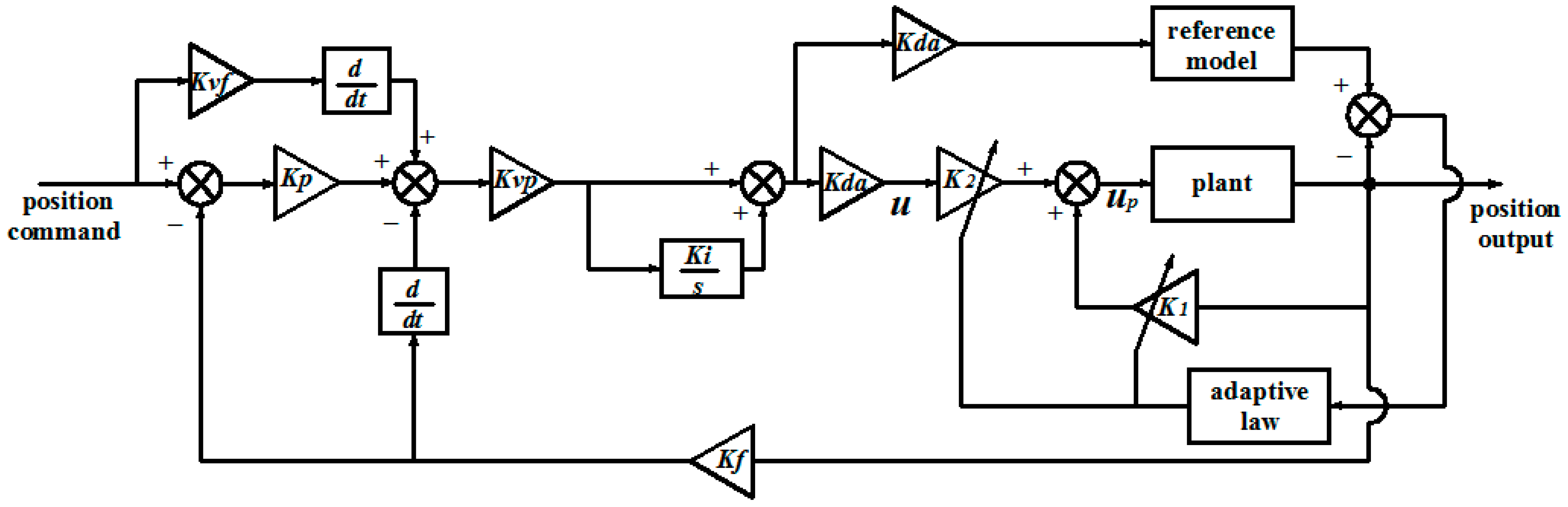
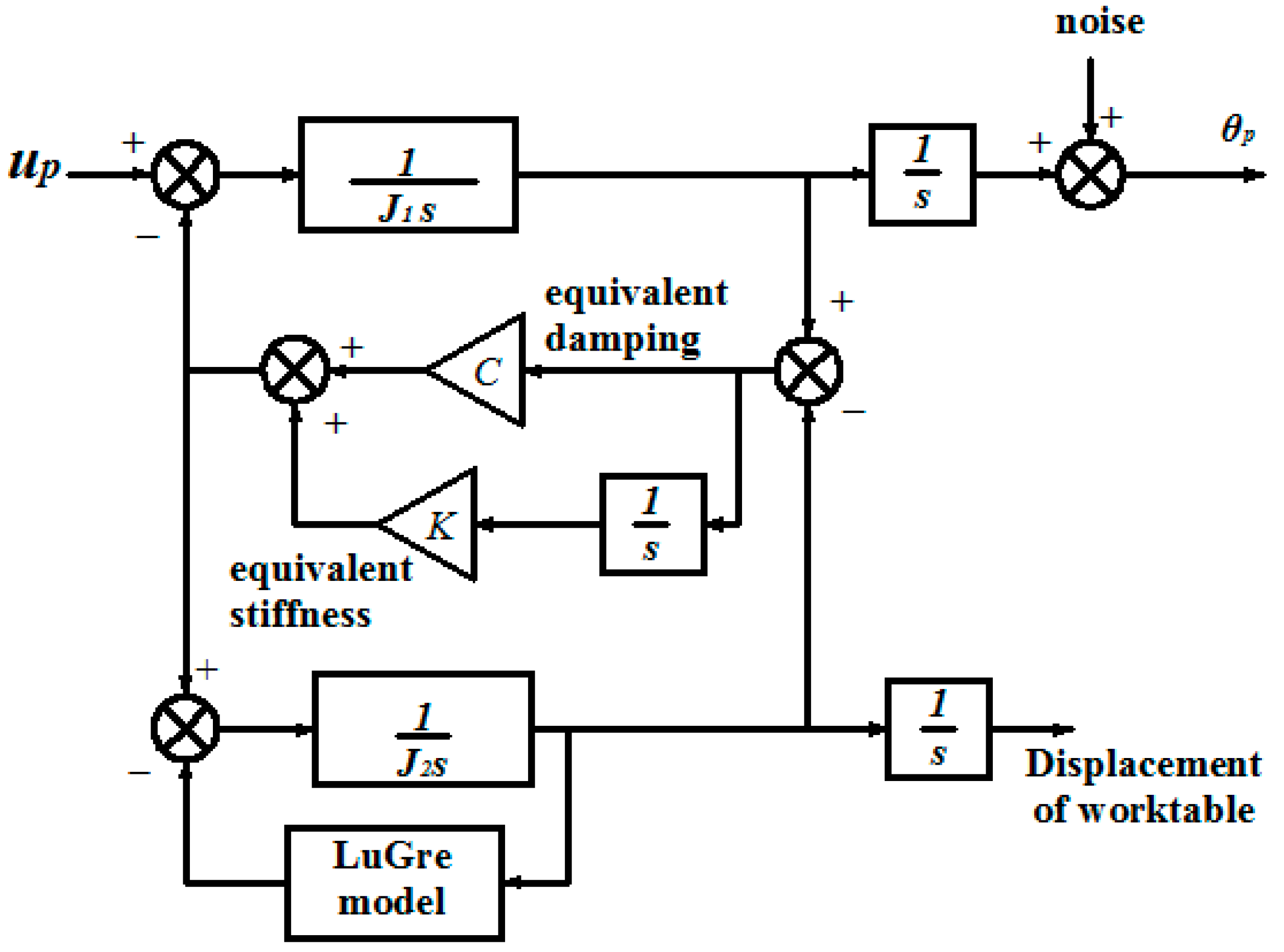
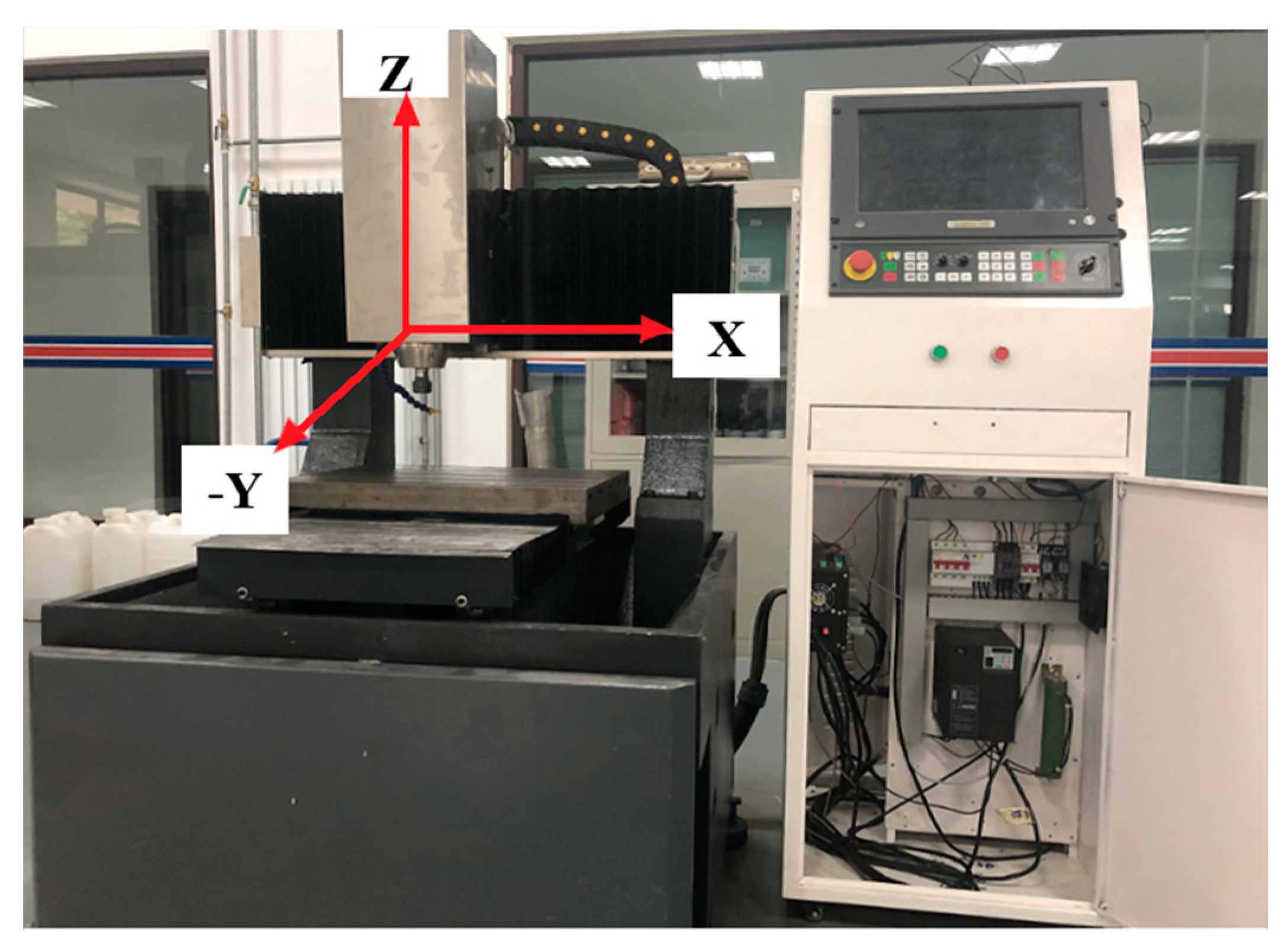
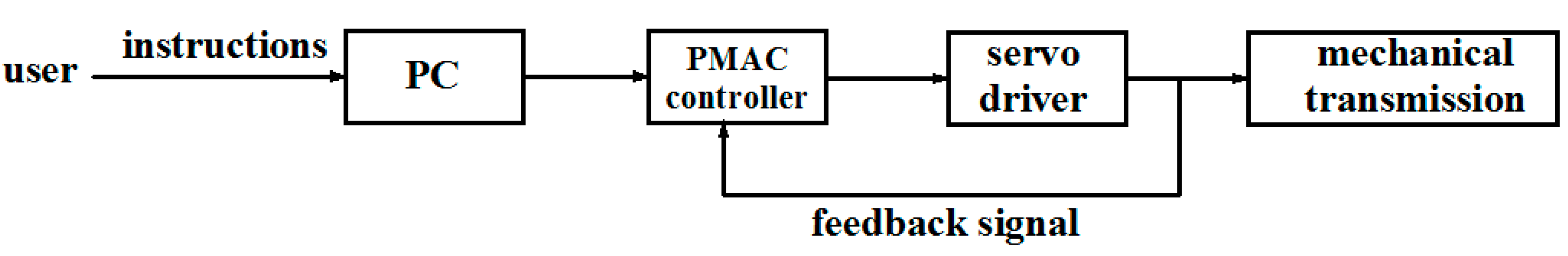
2. Framework of Feed Servo System

This paper refers to the control theory in [29], and establishes an adaptive control structure framework as shown in Figure 2, which includes a reference model, actual plant, the mechanism of adaptive law, and a parameter adjustable controller (constituted by K₁ and K₂). For MRAC, a generalized error is generated between the output of the plant and the reference model, and the error is used to adjust the controller parameters in real time, to minimize the error and improve the control performance of the system, especially for the control of nonlinear factors.

In Figure 2, u is the torque output of PID control; in the torque input of MRAC u_p, obtained by the adaptive adjustment of K₁ and K₂ as the input of the plant, the generalized error is used as the input signal of the mechanism of adaptive law to adaptively adjust the system.

On the above basis, the control framework has been built as shown in Figure 3, where Kp, Kvp and Kf correspond to the position loop gain, the speed loop gain, and the feedback gain. Ki is the integral gain, and Kvf is the speed feedforward gain. Kda is the coefficient of digital-to-analog conversion, which converts digital quantities into torque. In addition, the introduction of speed feedforward can reduce the linear error of PID control and improve the dynamic response capability of the system [30].

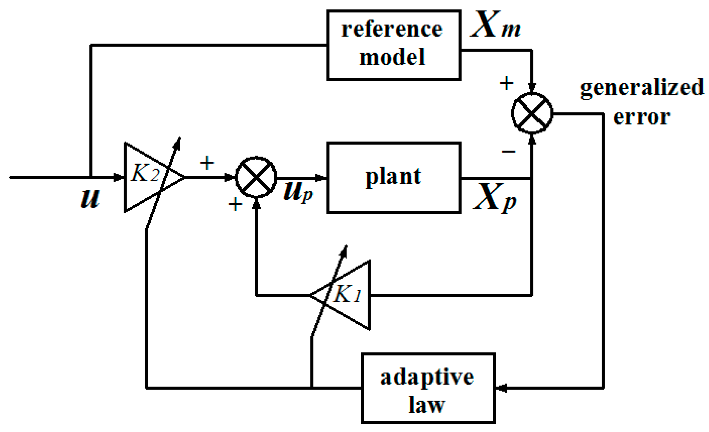
3. Establishment of Adaptive System

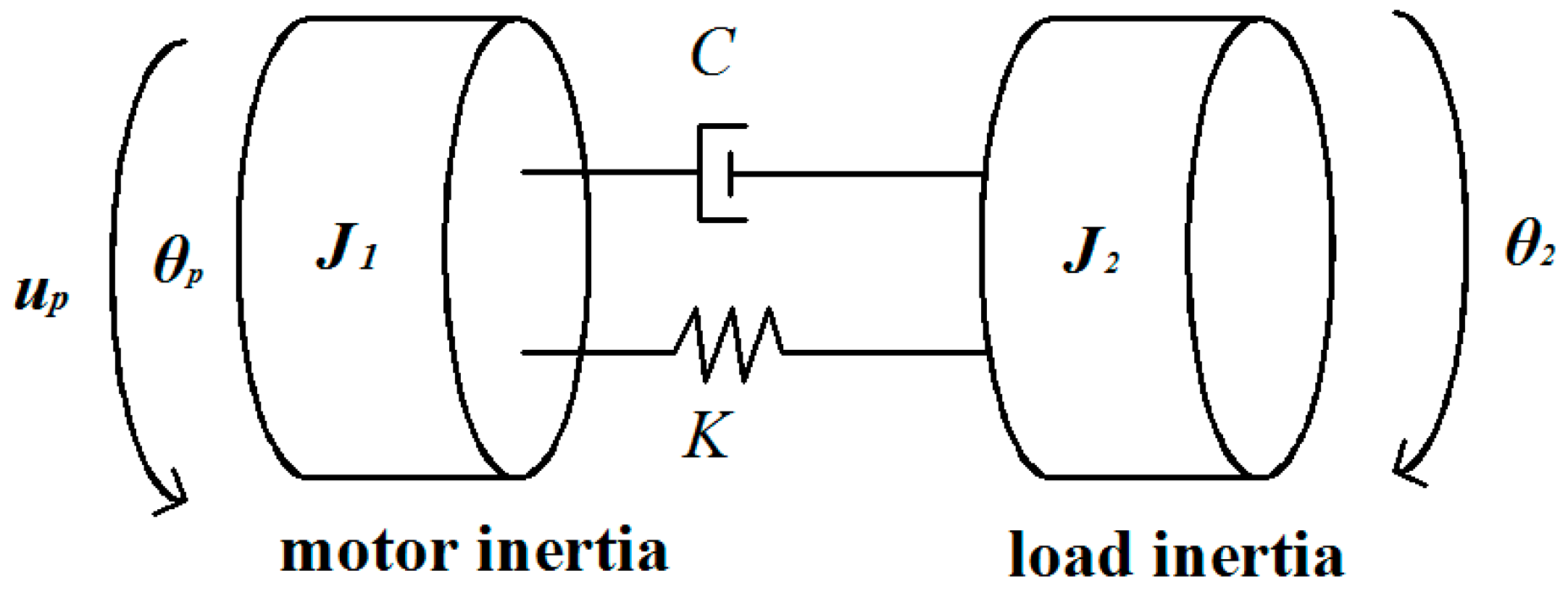
3.1. Model Definition and Deduction

Given the expression of the state equation:

$$\{\begin{array}{l}{\dot{X}}_p=A_p{X}_p+B_p{u}_p\\ Y_p=I{X}_p\end{array}$$

(1)

where $X_p$ is a 2 × 1 state vector, including the two state variables of motor angular displacement ${\theta }_p$ and angular velocity ${\omega }_p$, measured by the actual machine tool. $A_p$ is a 2 × 2 system matrix, $B_p$ is a 2 × 1 control matrix, and $I$ is an identity matrix.

The reference model is considered to be a single degree of freedom rotating rigid body with viscous damping, and the equation of state is:

$$\{\begin{array}{l}{\dot{X}}_m=A_m{X}_m+B_{m}u\\ Y_m=I{X}_m\end{array}$$

(2)

$$\{\begin{array}{l}{A}_m=\left[\begin{array}{cc}0& 1\\ 0& -b_m/J_m\end{array}\right]\\ B_m=\left[\begin{array}{c}0\\ 1/J_m\end{array}\right]\end{array}$$

(3)

$b_m$, $J_m$ are rotational viscous damping coefficient and total inertia, respectively. $K_1$, $K_2$ are the state feedback matrix and the input gain matrix:

$$K_1=\left[\begin{array}{cc}{k}_{11}& k_{12}\end{array}\right]$$

(4)

$$K_2=\left[k_2\right]$$

(5)

According to Figure 2:

$$u_p=K_1{X}_p+k_{2}u=k_{11}{\theta }_1+k_{12}{\omega }_1+k_{2}u$$

(6)

Substituting (6) into (1) to obtain:

$${\dot{X}}_p=(A_p+B_p{K}_1)X_p+(B_p{k}_2)u$$

(7)

During the operation of the system, parameters $K_1$ and $K_2$ were continuously adjusted until the system reaches a steady state. At this time, the output of the reference model was consistent with the actual model, and there was:

$$\{\begin{array}{l}{A}_p+B_p{K}_1*=A_m\\ B_p{k}_2*=B_m\end{array}$$

(8)

Among them, $K_1*$, $k_2*$ are the values of $K_1$, $k_2$ in the steady state.

Define the generalized error and derive the time derivative:

$$E=X_m-X_p=\left[\begin{array}{c}{\theta }_m-{\theta }_p\\ {\omega }_m-{\omega }_p\end{array}\right]$$

(9)

$$\begin{array}{l}\dot{E}={\dot{X}}_m-{\dot{X}}_p\\ =A_m{X}_m+B_{m}u-A_p{X}_p-B_p{u}_p\\ =A_{m}E+(A_m-A_p-B_p{K}_1)X_p+(B_m-B_p{k}_2)u\end{array}$$

(10)

Substituting (8) into (10):

$$\dot{E}=A_{m}E+\frac{B_m}{k_2*}(K_1*-K_1)X_p+\frac{B_m}{k_2*}(k_2*-k_2)u$$

(11)

Define the error of adaptive parameter and derive the time derivative:

$$\begin{array}{l}\{\begin{array}{l}{\widehat{K}}_1=K_1-K_1*\\ {\widehat{k}}_2=k_2-k_2*\end{array}\\ \{\begin{array}{l}{\dot{\widehat{K}}}_1={\dot{K}}_1\\ {\dot{\widehat{k}}}_2={\dot{k}}_2\end{array}\end{array}$$

(12)

Then, (11) is rewritten as:

$$\dot{E}=A_{m}E-\frac{B_m}{k_2*}{\widehat{K}}_1{X}_p-\frac{B_m}{k_2*}{\widehat{k}}_{2}u$$

(13)

3.2. Deduction of Adaptive Law Based on Lyapunov’s Stability Theory

The second method of Lyapunov stability theory is used to determine the adaptive law. Define the Lyapunov function as follows:

$$V(E,{\widehat{K}}_1{}^{{\rm T}},{\widehat{k}}_2)=E^{{\rm T}}PE+({\widehat{K}}_1\mathsf{\Psi }{\widehat{K}}_1{}^{{\rm T}}+\frac{1}{\alpha }{\widehat{k}}_2{}^2)$$

(14)

In (14), $P$, $\mathsf{\Psi }$ is a positive-definite symmetric matrix, and $\mathsf{\Psi }$ is simplified to $\left[\begin{array}{cc}{\psi }_1& 0\\ 0& {\psi }_2\end{array}\right]$, $\alpha >0$, obviously, $V$ is positive-definite.

Take the derivative of $V$ and substitute Equation (13) into:

$$\begin{array}{l}\dot{V}=E^{{\rm T}}{A}_M{}^{{\rm T}}PE+E^{{\rm T}}P{A}_{M}E\\ -\frac{2}{k_2*}{E}^{{\rm T}}P{B}_m{\widehat{K}}_1{X}_p-\frac{2}{k_2*}{E}^{{\rm T}}P{B}_m{\widehat{k}}_{2}u\\ +2{\widehat{K}}_1\mathsf{\Psi }{\dot{\widehat{K}}}_1{}^{{\rm T}}+\frac{2}{\alpha }{\widehat{k}}_2{\dot{\widehat{k}}}_2\end{array}$$

(15)

In (15), produce equation:

$$\{\begin{array}{l}2{\widehat{K}}_1\mathsf{\Psi }{\dot{\widehat{K}}}_1{}^{{\rm T}}-\frac{2}{k_2*}{E}^{{\rm T}}P{B}_m{\widehat{K}}_1{X}_p=0\\ \frac{2}{\alpha }{\widehat{k}}_2{\dot{\widehat{k}}}_2-\frac{2}{k_2*}{E}^{{\rm T}}P{B}_m{\widehat{k}}_{2}u=0\end{array}$$

(16)

Solve (16):

$$\{\begin{array}{l}{K}_1{}^{{\rm T}}=\frac{1}{k_2*}{\mathsf{\Psi }}^{-1}{\displaystyle \int (X_p{E}^{{\rm T}}P{B}_m)dt}+K_{c1}\\ k_2=\frac{\alpha }{k_2*}{\displaystyle \int (u{E}^{{\rm T}}P{B}_m)dt}+k_{c2}\end{array}$$

(17)

Integrate the constant parameters in (17), and produce

$$l_1=E^{{\rm T}}P{B}_m=(e_g{p}_{12}+{\dot{e}}_g{p}_{22})/J_m$$

(18)

Lastly, the adaptive law is:

$$\begin{array}{l}\{\begin{array}{l}{\dot{k}}_{11}={\gamma }_1\theta l_1\\ {\dot{k}}_{12}={\gamma }_2\omega l_1\\ {\dot{k}}_2={\gamma }_{3}u{l}_1\end{array}\\ \{\begin{array}{l}{k}_{11}={\gamma }_1{\displaystyle \int (\theta l_1)dt}+k_{c11}\\ k_{12}={\gamma }_2{\displaystyle \int (\omega l_1)dt}+k_{c12}\\ k_2={\gamma }_3{\displaystyle \int (u{l}_1)dt}+k_{c2}\end{array}\end{array}$$

(19)

${\gamma }_1$,${\gamma }_2$,${\gamma }_3$ are the corresponding adaptive law gains, $K_c{}_1={[k_c{}_{11}\hspace{1em}{k}_c{}_{12}]}^{\mathrm{T}}$ and $k_c{}_2$ are the corresponding initial values.

Then, (15) is rewritten as:

$$\dot{V}=E^{{\rm T}}{A}_M{}^{{\rm T}}PE+E^{{\rm T}}P{A}_{M}E$$

(20)

Define the Q matrix:

$$Q=A_m{}^{{\rm T}}P+P{A}_m$$

(21)

Substituting $A_m,P=\left[\begin{array}{cc}{p}_{11}& p_{12}\\ p_{21}& p_{22}\end{array}\right]$ into (21):

$$Q=\left[\begin{array}{cc}0& p_{11}-\frac{b_m}{J}{p}_{12}\\ p_{11}-\frac{B}{J_m}{p}_{21}& 2(p_{12}-\frac{b_m}{J_m}{p}_{22})\end{array}\right]$$

(22)

To make $\dot{V}<0$, this paper need to make the $Q$ matrix a negative-definite matrix. However, since the $A_m$ matrix has the characteristics of a singular matrix when it is initially defined, it is impossible to make the $Q$ matrix negative-definite. Therefore, make the $Q$ matrix a seminegative-definite matrix form; then, $\stackrel{.}{V}\le 0$.

$$Q=\lambda \left[\begin{array}{cc}0& 0\\ 0& -1\end{array}\right],\lambda >0$$

(23)

Lastly, the $P$ matrix needs to meet the following conditions:

$$\{\begin{array}{l}{p}_{11}=\frac{b_m}{J_m}{p}_{12}\\ p_{12}<\frac{bm}{J_m}{p}_{22}\end{array}$$

(24)

According to the second method of Lyapunov’s stability theory and the related conclusions derived above, $V(E,{\widehat{K}}_1{}^{{\rm T}},{\widehat{k}}_2)$ has a continuous first-order partial derivative and satisfies the following conditions:

1.

$V(0,0,0,)=0$;

2.

$V(E,{\widehat{K}}_1{}^{{\rm T}},{\widehat{k}}_2)$ is positive-definite;

3.

$\dot{V}(E,{\widehat{K}}_1{}^{{\rm T}},{\widehat{k}}_2)$ seminegative-definite.

Then, the system is stable in the sense of Lyapunov at the origin, that is, where the various errors are zero.

4. Simulation Experiment

4.1. Simulation Model

In MATLAB/Simulink, a simulation model of the control system was built as shown in Figure 3: the reference model is shown in Formula (2), and the two-inertia model is shown in the Figure 4, to replace the actual machine tool model. The differential equation of the two-inertia model is:

$$\begin{array}{l}{u}_p=J_1{\ddot{\theta }}_p+C\left({\dot{\theta }}_p-{\dot{\theta }}_2\right)+K\left({\theta }_p-{\theta }_2\right)\\ C\left({\dot{\theta }}_p-{\dot{\theta }}_2\right)+K\left({\theta }_p-{\theta }_2\right)=J_2{\ddot{\theta }}_2\end{array}$$

(25)

In Formula (25):

${\theta }_p$, ${\stackrel{.}{\theta }}_p$ and ${\ddot{\theta }}_p$ are angular displacement, angular velocity and angular acceleration of the servo motor.

${\theta }_2$, ${\dot{\theta }}_2$ and ${\ddot{\theta }}_2$ are displacement, velocity and acceleration of the worktable.

The simulation model is shown in Figure 5. Noise and LuGre model were added to approximate the actual situation.

Through the offline identification of dynamic parameters based on dual excitation signals, the characteristics of the two inertia models were obtained, and then the PID control gain was determined by the Ziegler-Nichols empirical method [31]. The speed feedforward gain was set to 1, to eliminate the influence of linear error as much as possible. The parameters of

Table 1. Relevant parameters of simulation model.

Name	Symbol	Value and Unit
Motor inertia	$J_1$	2.85 × 10–4 kg·m2
Load inertia	$J_2$	5.12 × 10–5 kg·m2
Equivalent stiffness	$K$	18.29 N·m/rad
Equivalent damping	$C$	0.064 N·m/rad
Total inertia	$J_m$	3.36 × 10–4 kg·m2
Viscous damping	$b_m$	0.014 N·m·s/rad
Position gain	$K_p$	0.051
Speed gain	$K_{vp}$	2.1
Integral gain	$K_i$	0.0146
Feedback gain	$K_f$	4,889,200
Coefficient of digital-to-analog conversion	$K_{da}$	3.1 × 10–5
Speed feedforward gain	$K_{vf}$	1
Sampling time	$T_0$	0.000408 s

were obtained through the above methods.

The friction model adopts the LuGre model [32], which can reflect well the static and dynamic characteristics of friction. The relationship between friction and speed is shown in the Formula (26) and Figure 6:

$$\{\begin{array}{l}s(V)=F_c+(F_s-F_c)e^{-{(V/V_s)}^2}\\ \dot{z}=v-\frac{{\sigma }_{0}z\left|V\right|}{s(V)}\\ F={\sigma }_{0}z+{\sigma }_{1}z+{\sigma }_{2}V\end{array}$$

(26)

In (26), $F_s$ is the maximal static friction; $F_c$ is the Coulomb friction; $z$ is the average elastic deformation of the bristles; ${\sigma }_0$ is the stiffness coefficient; ${\sigma }_1$ is the damping coefficient; ${\sigma }_2$ is the viscosity coefficient. As shown in

Table 2. Relevant parameters of friction model.

Name	Symbol	Value and Unit
Maximal static friction	$F_s$	0.04263 N/m
Coulomb friction	$F_c$	0.0091 N/m
Stribeck speed	$v_s$	0.007353 m/s
Stiffness coefficient	${\sigma }_0$	8.0274 N/m
Damping coefficient	${\sigma }_1$	2.343 N·s/m2
Viscosity coefficient	${\sigma }_2$	0.02772 N·s/m2

, the above parameters were obtained by the identification of friction parameters based on particle swarm algorithm [31].

The rotary model was regarded as the controlled object. The feedback signal and input signal are converted into digital quantities for calculation after sampling. The position and velocity data of the rotating model involved in the following have been processed.

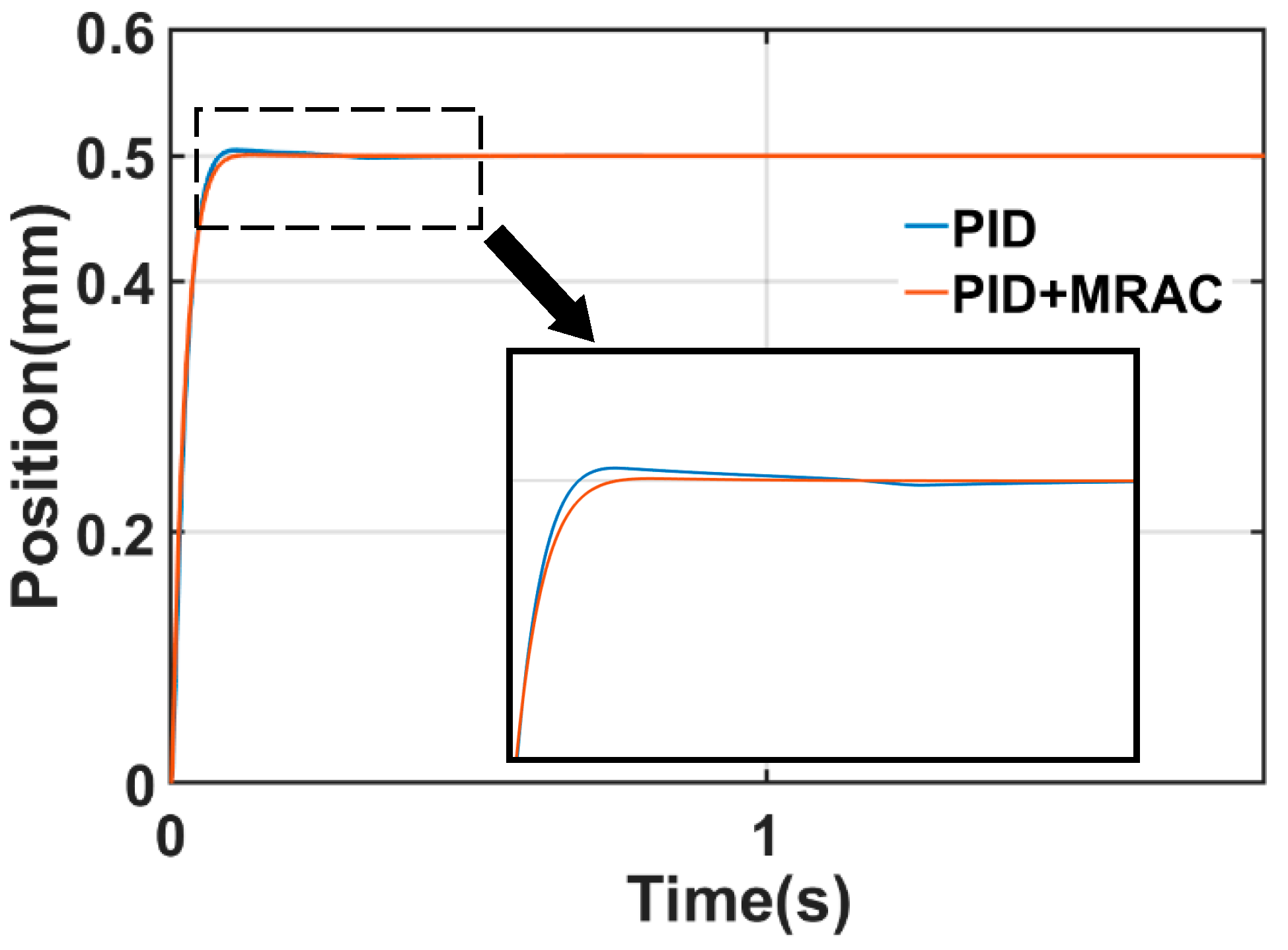
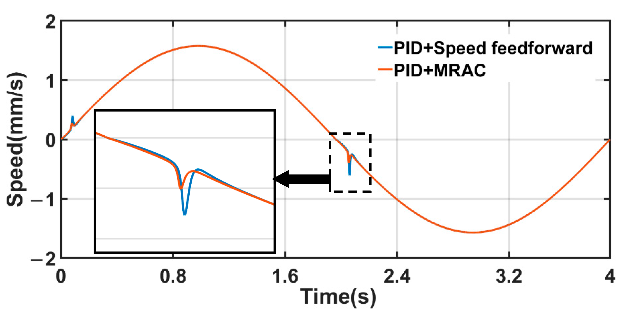
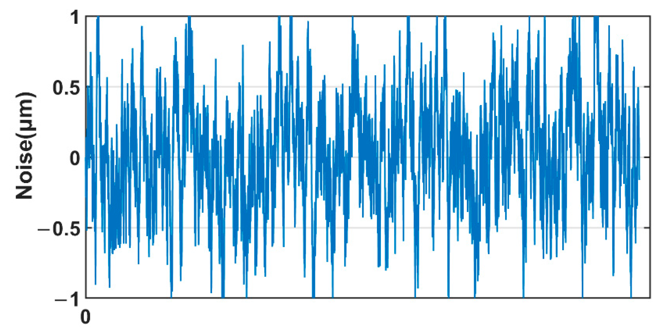
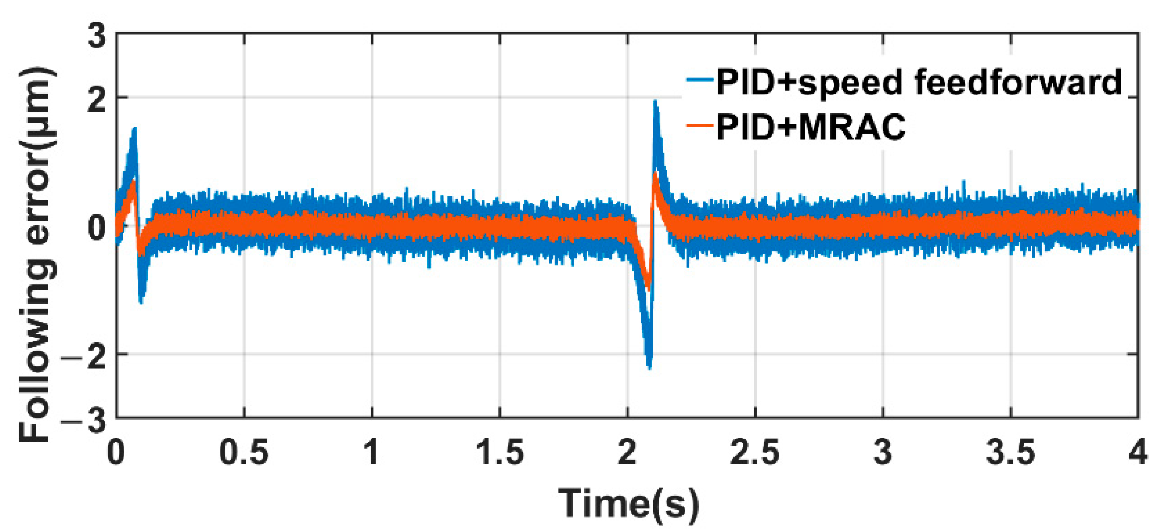
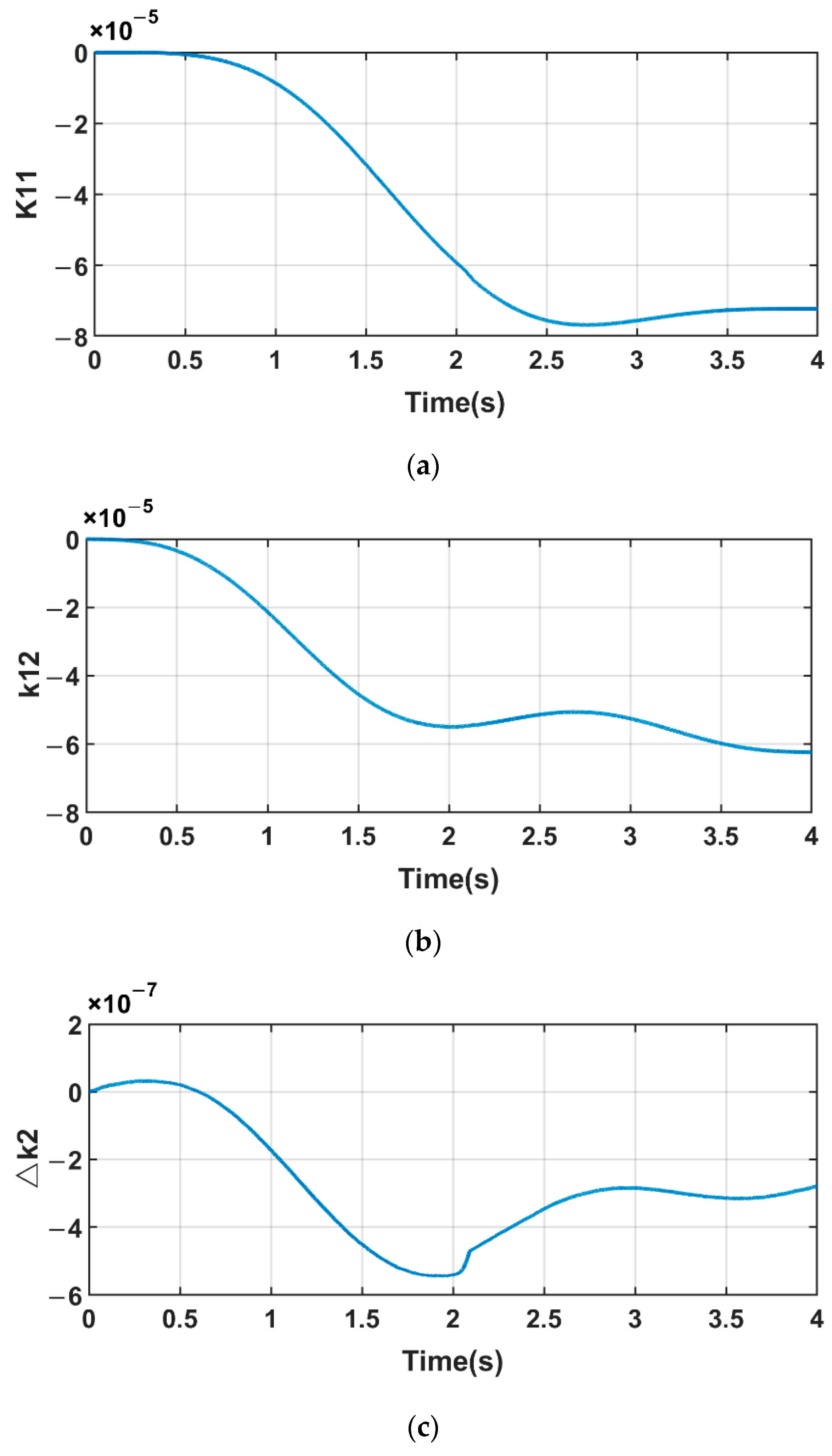
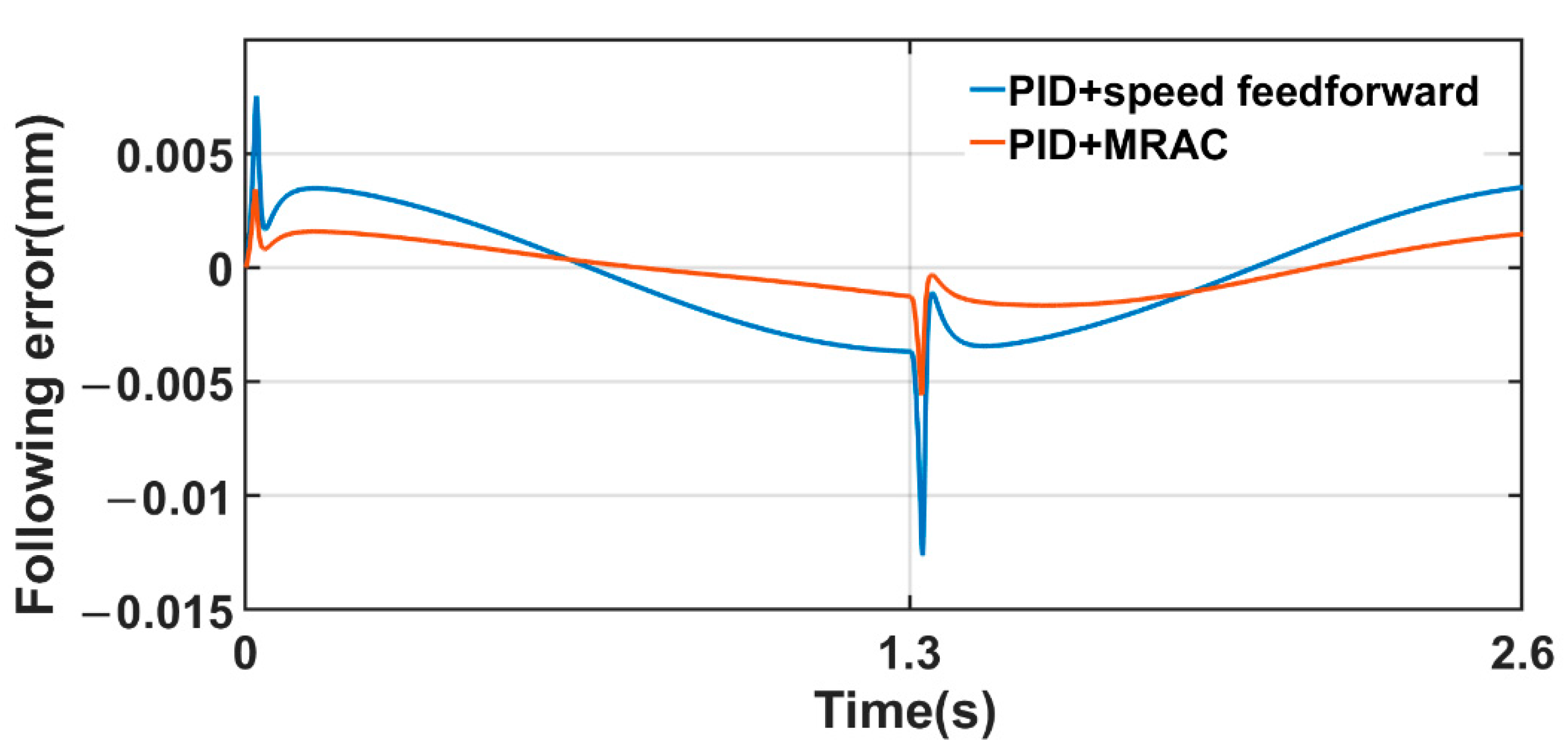
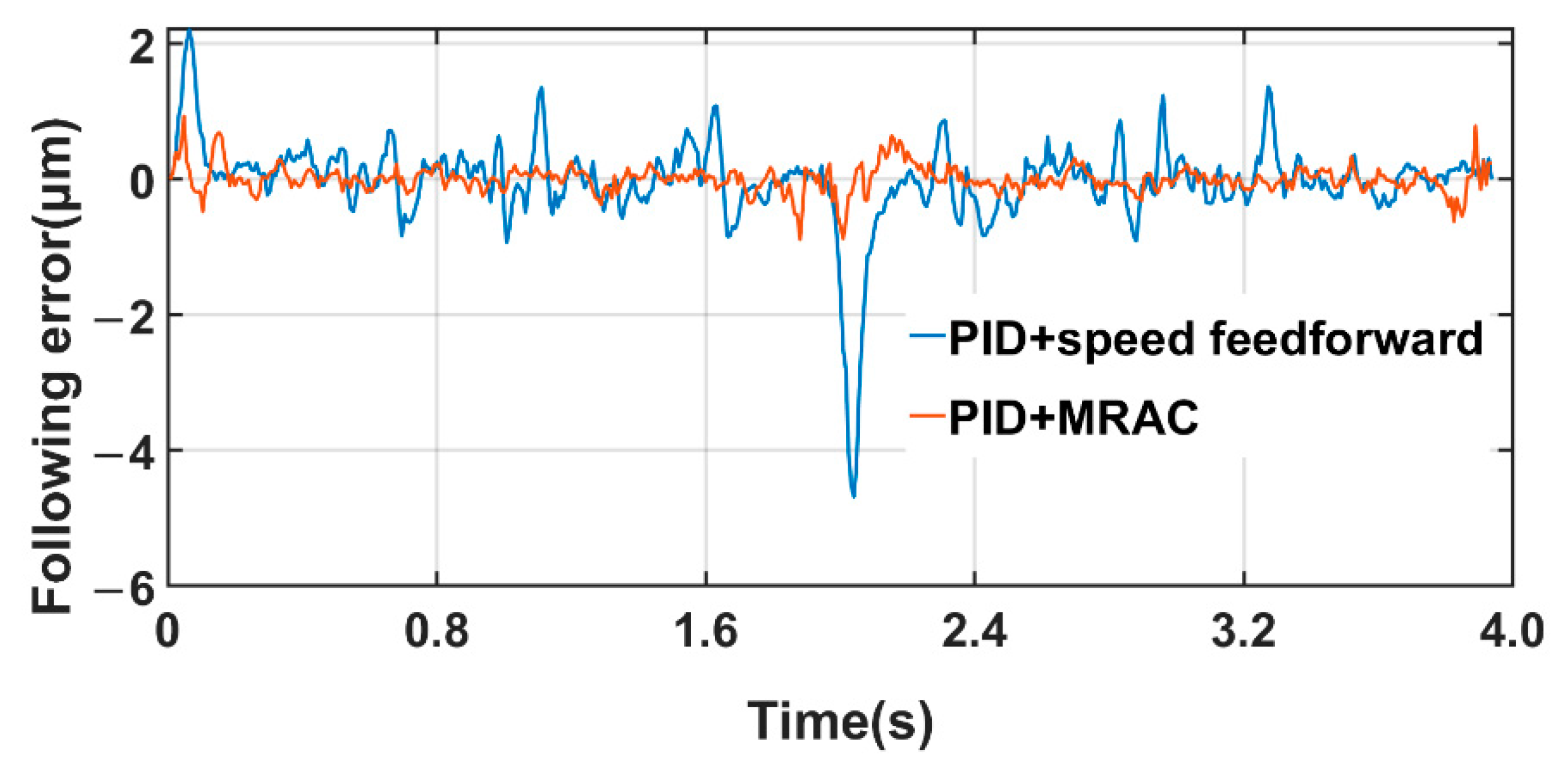
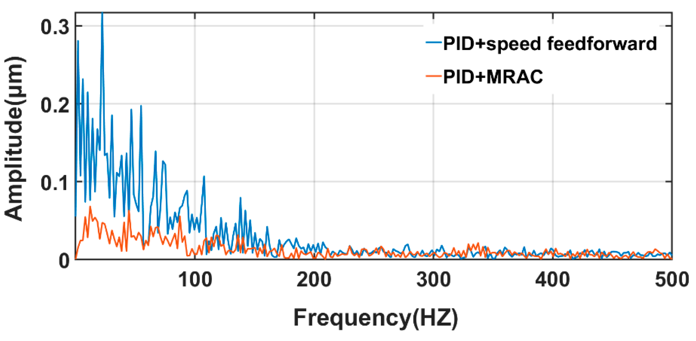
4.2. Simulation Analysis

To show the movement of the worktable more intuitively, the rotary motion needed to be transformed into translational motion. The angular displacement generated by the rotating model was converted into a linear displacement by the ball screw (lead is 5 mm), where every 2π rad of the rotary model rotates, the corresponding linear displacement is 5 mm.

In the adaptive control system simulation, according to the condition of Formula (24), let $p_{12}=1, p_{22}=1$, adaptive law gain ${\gamma }_1={\gamma }_2={\gamma }_3=1\times {10}^{-5}$. First, give the input position signal $r=-\cos (0.5\pi t)+1$ (unit is mm, at two seconds, the speed reversal). The signal curve is shown in Figure 7. Perform several simulations to determine the initial value of each adaptive law. After several simulations, the initial value is taken:

$$\{\begin{array}{l}{k}_{c11}=0\\ k_{c12}=0\\ k_{c2}=2.2\end{array}$$

Figure 8 shows the step response of 0.5 mm, after the appropriate initial value was determined, MRAC control could make the system response more stable and faster. The steady-state response time has been shortened from 0.537 s to 0.110 s and the speedability increased by 79.52%.

Figure 9 shows that, after using PID + MRAC control, the sinusoidal speed curve was closer to the desired speed curve. During speed reversal, the speed was less affected by nonlinear friction, which effectively reduced the error at the speed zero crossing. The sharp corner of the speed signal was reduced from 0.61 mm/s to 0.40 mm/s and the reduction was 34.43%, which shows that the PID + MRAC control could effectively weaken the influence of nonlinear friction.

To verify the role of MRAC in reducing noise, the position noise was added to the output of the servo motor. As shown in Figure 10, the noise was generated by the block of uniform random number and the value was generated randomly within a certain range. Position signal $r=-\cos (0.5\pi t)+1$ was used as input signal, followed by a simulation experiment.

Figure 11 shows that, compared with traditional PID + speed feedforward control, PID + MRAC could effectively reduce the excessive following error caused by nonlinear friction during speed reversal, the maximal error of 1.96 μm was reduced to 0.84 μm, and the reduction was 57.12%; on the other hand, it could also reduce the impact of noise.

Figure 12 shows the change of adjustable parameters. To make the data changes of k₂ more intuitive, it needs to be processed, so let:

$$\Delta k_2=k_2-k_{c2}=k_2-2.2$$

(27)

It can be seen from Figure 12 that the parameters change more slowly in the second half (from 2 s to 4 s) compared to the first half. In the initial response of the system, the friction and other factors have large changes, so the control parameters change relatively drastically.

According to the general machining speed of CNC, the input signal was defined as $r=-20\cos (\pi t/1.3)+20$ (unit is mm), followed by simulation experiment. As shown in Figure 13, when the processing speed was relatively fast, the introduction of MRAC not only effectively reduced the influence of friction on the following error (the maximal error of 12.62 μm was reduced to 5.60 μm, and the reduction was 55.63%) but also significantly improved the initial response speed. In addition, when the speed increased, the linear error caused by acceleration also increased accordingly, from the overall trend of the following error, PID+MRAC could still effectively reduce the linear error without introducing acceleration feedforward, and enhance the stability of the system. In general, when the speed was relatively fast, the control method proposed in this paper has more significant advantages in terms of rapidity, stability, and anti-interference compared with the traditional PID + speed feedforward control.

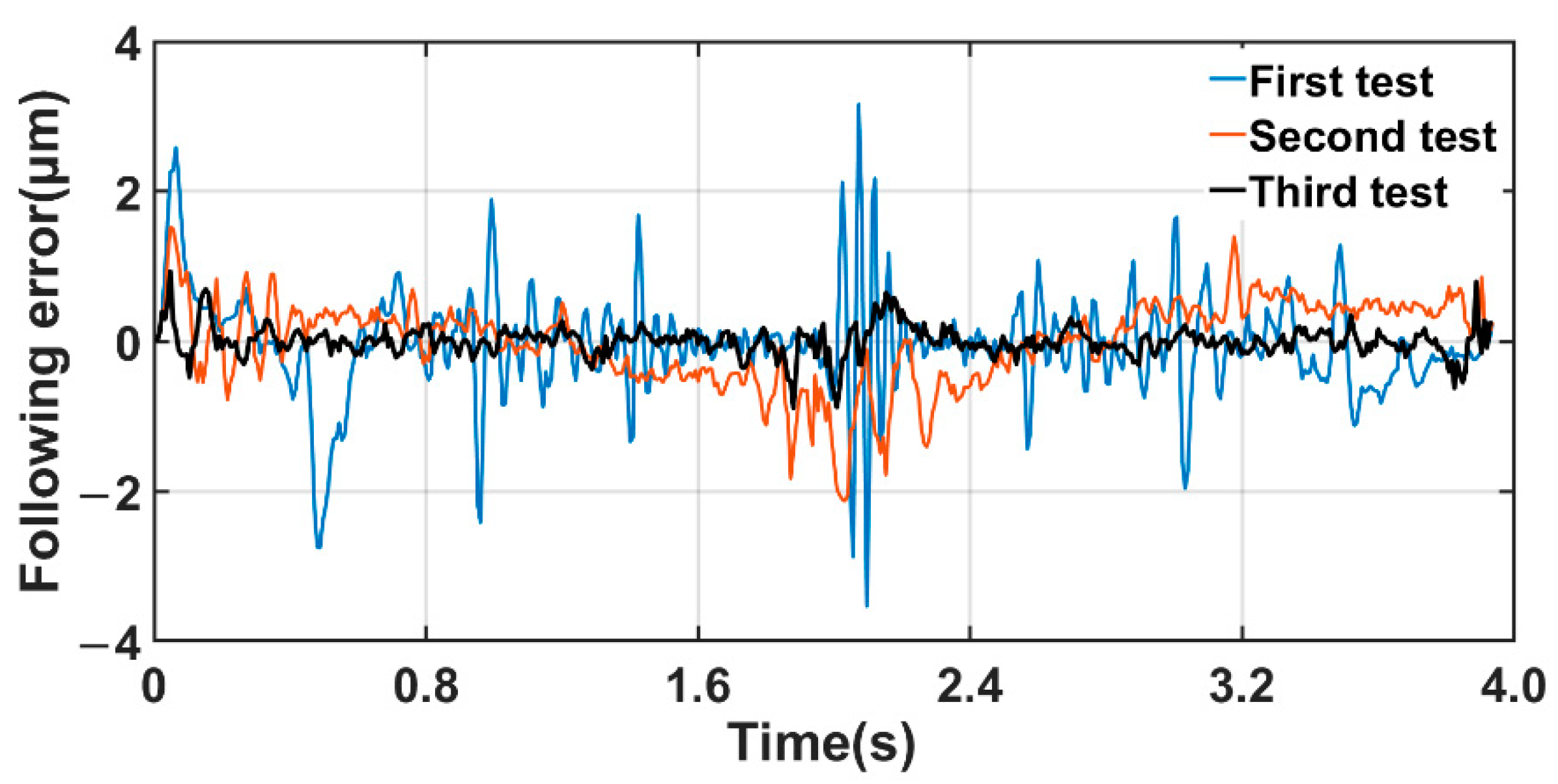
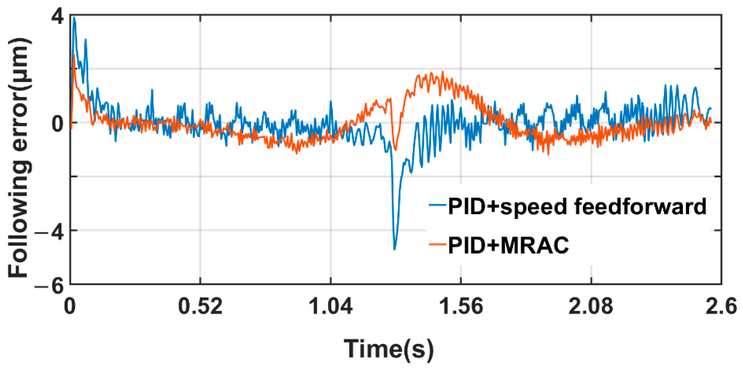
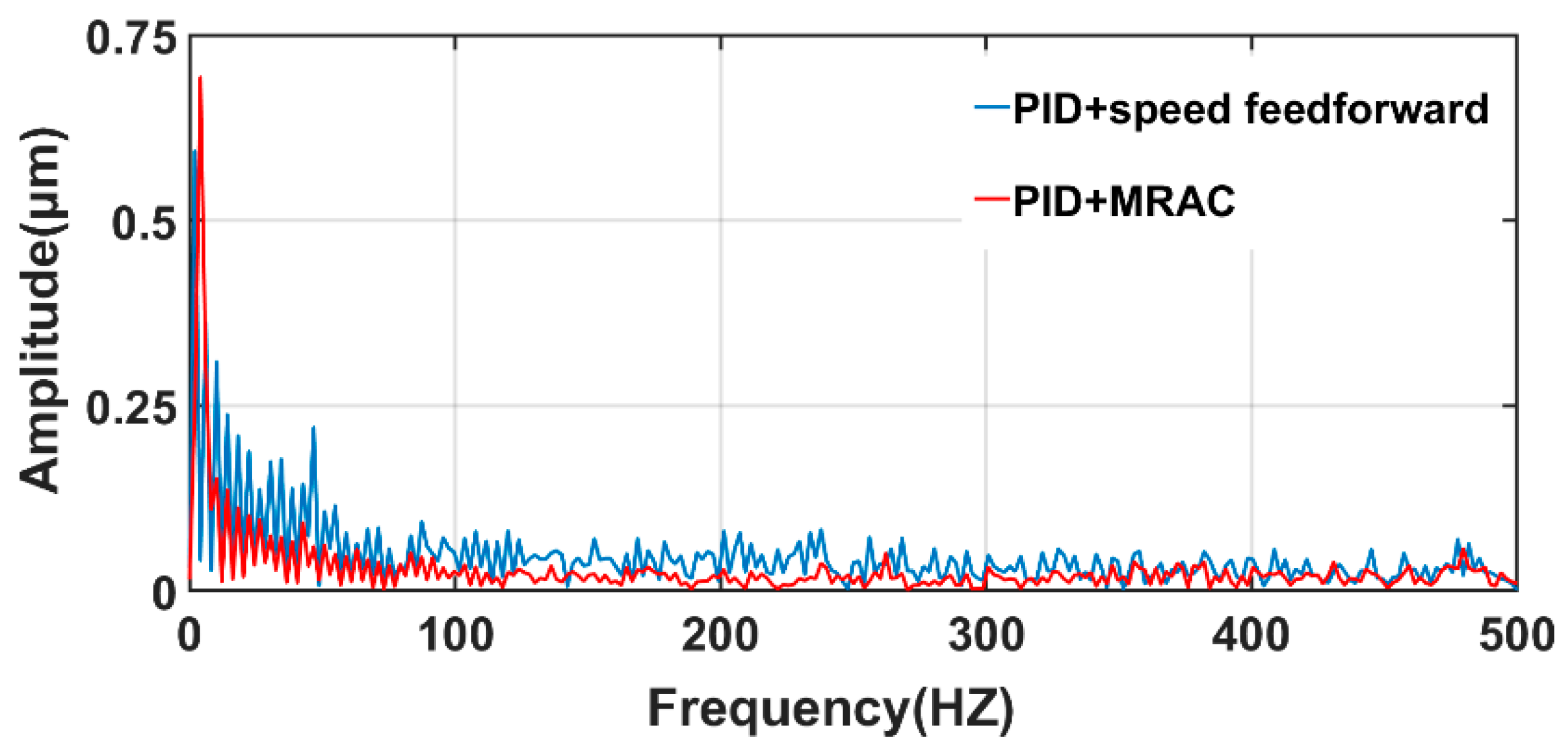
5. Experimental Verification

The experimental platform used in this article is shown in Figure 14, comprising a PMAC controller, PC, Yaskawa servo driver (SGD7S-5R500A002), and workbench. In PMAC, the servo operation was performed in units of digital cts (the conversion relationship is 1 mm = 2000 cts), and the drive was in torque control mode. Then, the reference model, adaptive algorithm, and PID control algorithm were written into the PMAC for experimental verification. Figure 15 is the frame diagram of the experimental platform. The feedback signal received by the PMAC controller comes from the encoder on the servo driver, so the whole system is a semi-closed-loop control system. The parameters and input signals used in this section are consistent with those of the model in Table 1. Research work only for the Y axis.

The sinusoidal speed signal was used as the test command for processing experiments. The average linear speed corresponding to circle processing was 1.57 mm/s, and the radius was 2 mm.

With the above test command as input, the processing experiment was performed three times in a row, and the following error is shown in Figure 16. The maximum following errors are 3.54 μm, 2.12 μm and 0.89 μm respectively. It can be seen that the following error of the system was continuously reduced under the effect of adaptive adjustment to obtain the best control performance.

The following error in Figure 17 shows that, during speed reversal, nonlinear friction caused excessive following error, especially under PID + speed feedforward control; when the control method proposed in this paper was used, the following error was greatly reduced: the maximal error of 4.685 μm was reduced to 0.89 μm, and the reduction was 81%. The initial response of the system was well optimized. The frequency spectrum of the following error was analyzed by fast Fourier transform. The sampling frequency was 1 KHZ. The analytical result in Figure 18 shows that the control strategy proposed in this paper could effectively reduce the resonance amplitude caused by mechanical transmission and noise.

To verify the applicability of the control method in this paper, the relatively fast sine speed command was used for the processing experiment (the average linear velocity of circle processing was 3 m/min, and the radius was 40 mm). Following error and error-spectrum analysis are shown in Figure 19 and Figure 20.

Figure 19 shows that the proposed control method could still reduce the excessive following error caused by nonlinear friction during speed reversal: during rapid processing, the maximal error of 4.715 μm was reduced to 1.895 μm, and the reduction was 59.81%. However, after the speed had been reversed, the error had a certain fluctuation. This may have been due to the faster processing speed, which led to some insufficient adaptive adjustment capabilities at this time. As shown in Figure 20, the fluctuation of the error curve was reflected in the first peak at the low frequency, but the amplitude at other frequencies was still effectively reduced. Although control performance was somewhat reduced, it could generally still effectively reduce the influence of nonlinear factors.

In general, compared with friction compensation, observer and filter, the control method proposed in this paper used relatively simple modeling and algorithms. Experiments showed that, through multiple runs, the control performance can be continuously improved. When the optimal control performance was achieved through adaptive adjustment, the control system could effectively reduce the influence of friction and noise at the same time. When the controlled object is changed, the control system will also change accordingly and the applicability and convenience are greatly improved.

6. Conclusions

In the mechanical transmission system of CNC, PID control cannot achieve better control performance because of various nonlinear factors. Therefore, in this paper, based on the advantages of PID, a new model reference adaptive control method based on PID control is proposed. The control framework was established and the adaptive law was obtained by Lyapunov stability theory. Through simulation analysis and experimental verification, and remarkable control results were obtained. Experimental results showed that the proposed model reference adaptive control based on PID control had an excellent control effect on the following error caused by nonlinear friction in the speed-reversal process (the proportion of reduction by more than 50%), had an effective suppression effect on noise and mechanical resonance, and at the same time improved the speed of response. When the processing speed was fast, although control performance was somewhat reduced, it still showed strong anti-interference ability. In addition, through the comparison between simulation and experiment, the effect of suppression of vibration in actual experiment became worse, which may be caused by the high-order and nonmodeling errors of the driving object. In general, this paper applied MRAC to CNC machine tools and obtained obvious research results with important practical engineering significance.

For the fluctuation in rapid processing, future work will focus on how to optimize the control method in this paper. At the same time, a detailed theoretical analysis of the stability of linear and nonlinear control combinations will also be considered.

References

1. Li, X.W. Study on Trajectory Error Prediction and Compensation Methods in High Speed Machining. Ph.D. Thesis, Xi’an Jiaotong University, Xi’an, China, 2013. [Google Scholar]
2. Huang, X.; Zhao, F.; Mei, X.; Tao, Y.; Tao, T.; Shi, H.; Liu, X. A novel triple-stage friction compensation for a feed system based on electromechanical characteristics. Precis. Eng. 2019, 56, 113–122. [Google Scholar] [CrossRef]
3. Keck, A.; Zimmermann, J.; Sawodny, O. Friction parameter identification and compensation using the ElastoPlastic friction model. Mechatronics 2017, 47, 168–182. [Google Scholar] [CrossRef]
4. Brock, S.; Łuczak, D.; Nowopolski, K.; Pajchrowski, T.; Zawirski, K. Two Approaches to Speed Control for Multi-Mass System with Variable Mechanical Parameters. IEEE Trans. Ind. Electron. 2017, 64, 3338–3347. [Google Scholar] [CrossRef]
5. Wang, W.; Xu, J.; Shen, A. Detection and reduction of middle frequency resonance for an industrial servo. In Proceedings of the 2012 IEEE International Conference on Information Science and Technology, Wuhan, China, 23–25 March 2012; Volume 21, pp. 899–907. [Google Scholar]
6. Sun, J.; Wang, C.; Xin, R. Anti-Disturbance Study of Position Servo System Based on Disturbance Observer. IFAC-PapersOnLine 2018, 51, 202–207. [Google Scholar] [CrossRef]
7. Whitaker, H.; Yamron, J.; Kezer, A. Design of Model Reference Adaptive Control Systems for Aircraft; MIT Press: Cambridge, MA, USA, 1958. [Google Scholar]
8. Zhang, D.; Wei, B. A review on model reference adaptive control of robotic manipulators. Annu. Rev. Control 2017, 43, 188–198. [Google Scholar] [CrossRef]
9. Shekhar, A.; Sharma, A. Review of model reference adaptive control. In Proceedings of the 2018 International Conference on Information, Communication, Engineering and Technology (ICICET), Pune, India, 29–31 August 2018. [Google Scholar]
10. Koksal, M.; Yenici, F.; Asya, A.N. Position Control of a Permanent Magnet DC Motor by Model Reference Adaptive Control. In Proceedings of the 2007 IEEE International Symposium on Industrial Electronics, Vigo, Spain, 4–7 June 2007. [Google Scholar]
11. Guo, L.; Parsa, L. Model Reference Adaptive Control of Five-Phase IPM Motors Based on Neural Network. In Proceedings of the 2011 IEEE International Electric Machines & Drives Conference (IEMDC), Niagara Falls, ON, Canada, 15–18 May 2011. [Google Scholar]
12. Abo-Khalil, A.G.; Eltamaly, A.M.; Alsaud, M.S.; Sayed, K.; Alghamdi, A.S. Sensorless control for PMSM using model reference adaptive system. Int. Trans. Electr. Energy 2020, 31, 31. [Google Scholar]
13. Gruenwald, B.C.; Yucelen, T.; Muse, J.A. Direct Uncertainty Minimization Framework for System Performance Improvement in Model Reference Adaptive Control. Machines 2017, 5, 9. [Google Scholar] [CrossRef] [Green Version]
14. Abdelrahem, M.; Hackl, C.M.; Kennel, R. Limited-Position Set Model-Reference Adaptive Observer for Control of DFIGs without Mechanical Sensors. Machines 2020, 8, 72. [Google Scholar] [CrossRef]
15. Crnosija, P.; Ban, Z.; Krishnan, R. Application of model reference adaptive control with signal adaptation to PM brushless DC motor drives. In Proceedings of the 2002 IEEE International Symposium on Industrial Electronics (ISIE), L’Ayuila, Italy, 8–11 July 2002. [Google Scholar]
16. Shi, C.; Wang, C. Sensorless Vector Control of Three-Phase Permanent Magnet Synchronous Motor Based on Model Reference Adaptive System. In Proceedings of the 4th International Conference on Control Science and Systems Engineering (ICCSSE), Wuhan, China, 21–23 August 2018. [Google Scholar]
17. Nour, M.; Aris, I.; Mariun, N.; Mahmoud, S. Hybrid Model Reference Adaptive Speed Control for Vector Controlled Permanent Magnet Synchronous Motor Drive. In Proceedings of the 2005 International Conference on Power Electronics and Drives Systems, Kuala Lumpur, Malaysia, 28 November–1 December 2005. [Google Scholar]
18. Jiang, J.; Zhou, X.; Zhao, W.; Li, W. A model reference adaptive sliding mode control for the position control of permanent magnet synchronous motor. Proc. Inst. Mech. Eng. 2021, 235, 389–399. [Google Scholar] [CrossRef]
19. Yao, Z.; Yao, J.; Yao, F.; Xu, Q.; Xu, M.; Deng, W. Model reference adaptive tracking control for hydraulic servo systems with nonlinear neural-networks. ISA Trans. 2020, 100, 396–404. [Google Scholar] [CrossRef] [PubMed]
20. Ma, J.; Zhang, R.H. Model Reference Adaptive Neural Sliding Mode Control for Aero-Engine. AASRI Procedia 2012, 3, 508–514. [Google Scholar] [CrossRef]
21. Rajesh, R.; Deepa, S.N. Design of direct MRAC augmented with 2 DoF PIDD controller: An application to speed control of a servo plant. J. King Saud Univ. Sci. 2020, 32, 310–320. [Google Scholar] [CrossRef]
22. Guo, R.; Chen, J.; Hao, X. Position servo control of a DC electromotor using a hybrid method based on model reference adaptive control (MRAC). In Proceedings of the 2010 International Conference on Computer, Mechatronics, Control and Electronic Engineering, Changchun, China, 24–26 August 2010. [Google Scholar]
23. Dey, R.; Jain, S.; Padhy, P. Robust closed loop reference MRAC with PI compensator. IET Control Theory Appl. 2016, 10, 2378–2386. [Google Scholar] [CrossRef]
24. Pravika, M.; Jacob, J.; Joseph, K.P. Design of model reference adaptive–PID controller for automated portable duodopa pump in Parkinson’s disease patients. Biomed. Signal Process. Control. 2021, 68, 102590. [Google Scholar]
25. Zhang, J.; Ma, X.; Wang, Y.; Zhang, Z.; Wu, X. Application of Model Reference Adaptive PID Control in Magnetic Bearings. Bearing 2017, 4, 35–38. [Google Scholar]
26. Zhou, X.; Chao, Y.; Cai, T. A Model Reference Adaptive Control/PID Compound Scheme on Disturbance Rejection for an Aerial Inertially Stabilized Platform. J. Sens. 2016, 2016, 7964727. [Google Scholar] [CrossRef] [Green Version]
27. Zafari, Y.; Shoja-Majidabad, S. Sensorless fault-tolerant control of five-phase IPMSMs via model reference adaptive systems. Automatika 2020, 61, 564–573. [Google Scholar] [CrossRef]
28. Jung, J.-W.; Leu, V.Q.; Do, T.; Kim, E.-K.; Choi, H.H. Adaptive PID Speed Control Design for Permanent Magnet Synchronous Motor Drives. IEEE Trans. Power Electron. 2014, 30, 900–908. [Google Scholar] [CrossRef]
29. Coman, S.; Boldisor, C. Model Reference Aadptive Control for a DC Electrical Drive. Bull. Transilv. Univ. Brasov. Eng. Sci. Ser. 2013, 6, 33–38. [Google Scholar]
30. Liu, H.X.; Li, S.H. Speed Control for PMSM Servo System Using Predictive Functional Control and Extended State Observer. IEEE Trans. Ind. Electron. Control Instrum. 2012, 59, 1171–1183. [Google Scholar] [CrossRef]
31. Kong, L.Y. Development of System Identification Module for Three Axis Engraving and Milling Machine Based on PMAC. Master’s Thesis, Shandong University of Technology, Zibo, China, 2021. [Google Scholar]
32. De Wit, C.C.; Olsson, H.; Astrom, K.; Lischinsky, P. A new model for control of systems with friction. IEEE Trans. Autom. Control 1995, 40, 419–425. [Google Scholar] [CrossRef] [Green Version]
Figure 1. Effect of friction on control performance. (a) Speed “zero crossing”; (b) over-quadrant sharp corners.
Machines 09 00274 g001
Figure 2. MRAC system.
Machines 09 00274 g002
Figure 3. MRAC framework based on PID control.
Machines 09 00274 g003
Figure 4. Two-inertia model.
Machines 09 00274 g004
Figure 5. Block diagram of the two-inertia model.
Machines 09 00274 g005
Figure 6. Relationship between friction and velocity.
Machines 09 00274 g006
Figure 7. Curve of input signal: (a) desired position signal; (b) desired speed signal.
Machines 09 00274 g007
Figure 8. Step response of 0.5 mm.
Machines 09 00274 g008
Figure 9. Comparison of the speed of two methods.
Machines 09 00274 g009
Figure 10. Position noise.
Machines 09 00274 g010
Figure 11. Comparison of the following error of two methods.
Machines 09 00274 g011
Figure 12. Variation curve of adjustable parameters. (a) Variation of k11; (b) variation of k12; (c) variation of Δk2.
Machines 09 00274 g012
Figure 13. Comparison of the following error of two methods at general machining speed.
Machines 09 00274 g013
Figure 14. Experiment platform.
Machines 09 00274 g014
Figure 15. Frame diagram of experimental platform.
Machines 09 00274 g015
Figure 16. Following error of three processing experiments.
Machines 09 00274 g016
Figure 17. Comparison of following error of the two methods.
Machines 09 00274 g017
Figure 18. Frequency-spectrum analysis of following error.
Machines 09 00274 g018
Figure 19. Comparison of following error of the two methods.
Machines 09 00274 g019
Figure 20. Frequency-spectrum analysis of following error.
Machines 09 00274 g020