
Verification of a Body Freedom Flutter Numerical Simulation Method Based on Main Influence Parameters


Abstract
:1. Introduction
2. The Rigid–Elastic Coupled Dynamic Modeling Method: Taking a Two-Dimensional Airfoil as an Example
3. CFD and Fluid–Solid Coupling Calculation Method
4. CFD and Fluid–Solid Coupling Calculation Method
4.1. Results and Discussion of the Two-Dimensional Model
4.1.1. Model Parameters
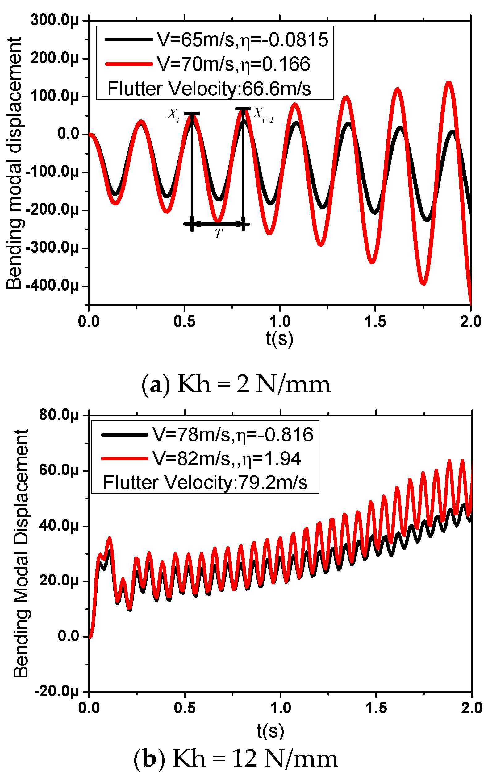
4.1.2. Numerical Solution by the CFD Method
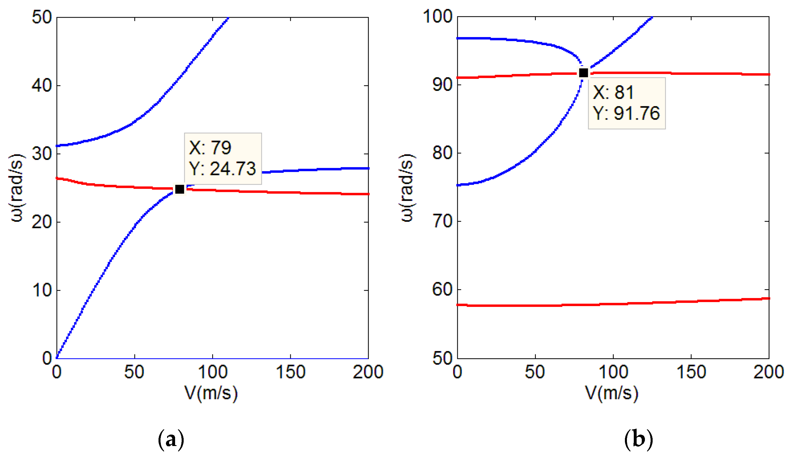
4.1.3. Theoretical Solution by the Theodorsen Unsteady Aerodynamic Model
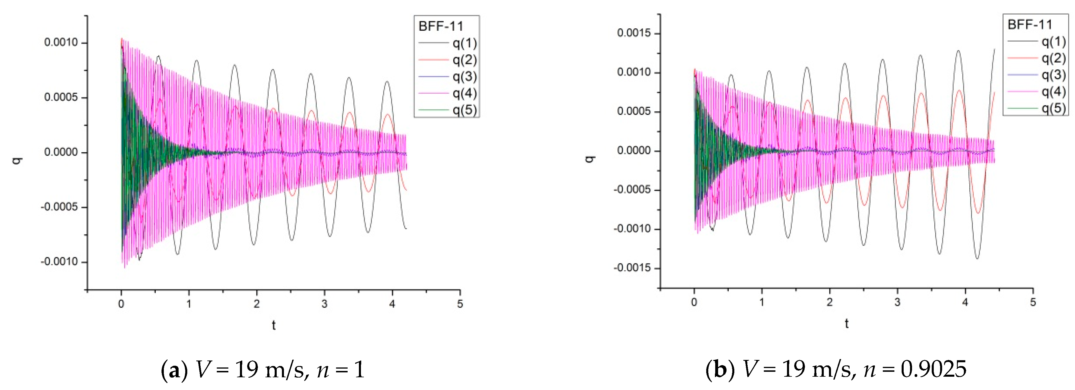
4.1.4. Discussion and Validation of the BFF Calculation Method Using a Navier–Stokes Fluid Model
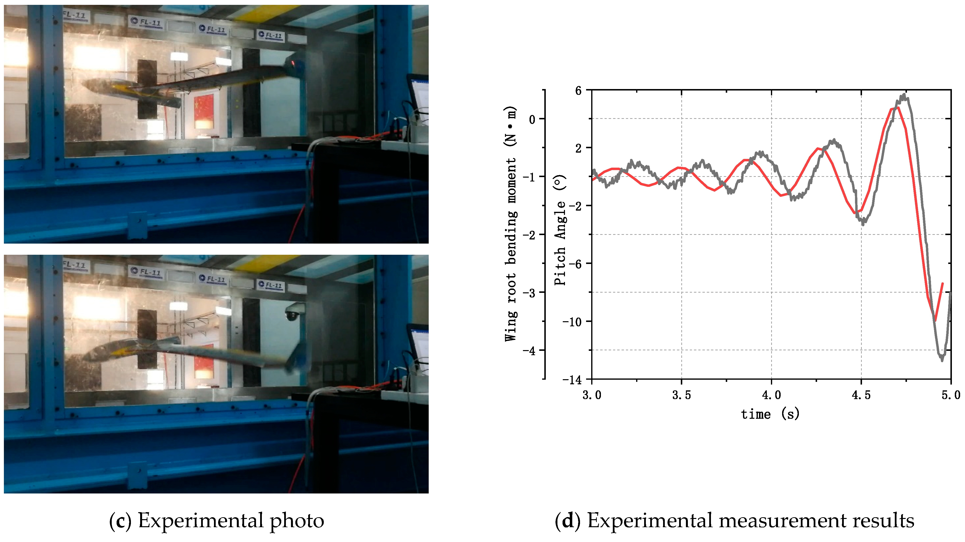
4.2. Results and Discussion of the Three-Dimensional Model
5. Conclusions
Author Contributions
Funding
Institutional Review Board Statement
Informed Consent Statement
Data Availability Statement
Conflicts of Interest
References
- Goh, G.D.; Agarwala, S.; Goh, G.L.; Dikshit, V.; Sing, S.L.; Yeong, W.Y. Additive manufacturing in unmanned aerial vehicles (UAVs): Challenges and potential. Aerosp. Sci. Technol. 2017, 63, 140–151. [Google Scholar] [CrossRef]
- Lv, B.B.; Lu, Z.L.; Guo, T.Q.; Tang, D.; Yu, L.; Guo, H.T. Investigation of winglet on the transonic flutter characteristics for a wind tunnel test model CHNT-1. Aerosp. Sci. Technol. 2019, 86, 430–437. [Google Scholar] [CrossRef]
- Delfrate, J.H. Helios Prototype Vehicle Mishap: Technical Findings, Recommendations, and Lessons Learned; Non-Linear Aeroelastic Tools Workshop: Alexandria, VA, USA, 2008. [Google Scholar]
- Guo, S.; Jing, Z.W.; Li, H.; Lei, W.T.; He, Y.Y. Gust response and body freedom flutter of a flying-wing aircraft with a passive gust alleviation device. Aerosp. Sci. Technol. 2017, 70, 277–285. [Google Scholar] [CrossRef] [Green Version]
- Yang, C.; Huang, C.; Wu, Z.G.; Tang, C.H. Progress and challenges for aeroservoelasticity research. Acta Aeronaut. ET Astronaut. Sin. 2015, 36, 1011–1033. [Google Scholar] [CrossRef]
- Love, M.H.; Wieselmann, P.; Youngren, H. Body Freedom Flutter of High Aspect Ratio Flying Wings. In Proceedings of the 46th AIAA/ASME/ASCE/AHS/ASC Structures, Structural Dynamics and Materials Conference, AIAA Paper 2005-1947, Austin, TX, USA, 18–21 April 2005. [Google Scholar] [CrossRef]
- Burnett, E.L.; Atkinson, C.; Beranek, J.; Sibbitt, B.; Holm-Hansen, B.; Nicolai, L. NDOF Simulation Model for Flight Control Development with Flight Test Correlation. In Proceedings of the AIAA Modeling & Simulation Technologies Conference, Toronto ON, Canada, 2–5 August 2010. [Google Scholar] [CrossRef]
- Moreno, C.P.; Seiler, P.J.; Balas, G.J. Model Reduction for Aeroservoelastic Systems. J. Aircr. 2014, 51, 280–290. [Google Scholar] [CrossRef] [Green Version]
- Pak, C.-G.; Truong, S. Creating a Test-Validated Finite-Element Model of the X-56A Aircraft Structure. J. Aircr. 2015, 52, 1644–1667. [Google Scholar] [CrossRef] [Green Version]
- Jones, J.; Cesnik, C.E. Nonlinear Aeroelastic Analysis of the X-56 Multi-Utility Aeroelastic Demonstrator. In Proceedings of the Dynamics Specialists Conference, San Diego, CA, USA, 4–8 January 2016. [Google Scholar] [CrossRef] [Green Version]
- Li, W.W.; Pak, C.-G. Mass Balancing Optimization Study to Reduce Flutter Speeds of the X-56A Aircraft. J. Aircr. 2015, 52, 1359–1365. [Google Scholar] [CrossRef]
- Mardanpour, P.; Hodges, D.H.; Neuhart, R.; Graybeal, N. Engine Placement Effect on Nonlinear Trim and Stability of Flying Wing Aircraft. J. Aircr. 2013, 50, 1716–1725. [Google Scholar] [CrossRef]
- Richards, P.W.; Yao, Y.; Herd, R.A.; Hodges, D.H.; Mardanpour, P. Effect of Inertial and Constitutive Properties on Body-Freedom Flutter for Flying Wings. J. Aircr. 2016, 53, 756–767. [Google Scholar] [CrossRef]
- Regan, C.D.; Taylor, B.R. mAEWing1: Design, Build, Test. In Proceedings of the AIA Atmospheric Flight Mechanics Conference, San Diego, CA, USA, 4–8 January 2016. [Google Scholar] [CrossRef]
- Huang, C.; Wu, Z.G.; Yang, C.; Dai, Y.T. Flutter Boundary Prediction for a Flying-Wing Model Exhibiting Body Freedom Flutter. In Proceedings of the 58th AIAA/ASCE/AHS/ASC Structures, Structural Dynamics, and Materials Conference, Grapevine, TX, USA, 9–13 January 2017; p. 0415. [Google Scholar] [CrossRef]
- Huang, C.; Yang, C.; Wu, Z.; Tang, C. Variations of flutter mechanism of a span-morphing wing involving rigid-body motions. Chin. J. Aeronaut. 2018, 31, 490–497. [Google Scholar] [CrossRef]
- Li, Y.D.; Zhang, X.P.; Gu, Y.S.; Yang, Z.C. Body Freedom Flutter Study and Passive Flutter Suppression for a High Aspect Ratio Flying Wing Model. Appl. Mech. Mater. 2014, 608–609, 708–712. [Google Scholar] [CrossRef]
- Gu, Y.; Yang, Z.; He, S. Body Freedom Flutter of a Blended Wing Body Model Coupled with Flight Control System. Procedia Eng. 2015, 99, 46–50. [Google Scholar] [CrossRef] [Green Version]
- Gao, C.; Zhang, W.; Ye, Z. Reduction of transonic buffet onset for a wing with activated elasticity. Aerosp. Sci. Technol. 2018, 77, 670–676. [Google Scholar] [CrossRef]
- Sodja, J.; Roizner, F.; De Breuker, R.; Karpel, M. Experimental characterisation of flutter and divergence of 2D wing section with stabilised response. Aerosp. Sci. Technol. 2018, 78, 542–552. [Google Scholar] [CrossRef]
- Waszak, M.R.; Schmidt, D.K. Flight dynamics of aeroelastic vehicles. J. Aircr. 1988, 25, 563–571. [Google Scholar] [CrossRef]
- Buttrill, C.S.; Zeiler, T.A.; Arbuckle, P.D. Nonlinear simulation of a flexible aircraft in maneuvering flight. In Proceedings of the Flight Simulation Technologies Conference, Monterey, CA, USA, 17–19 August 1987; pp. 17–19. [Google Scholar] [CrossRef]
- Meirovitch, L. Hybrid state equations of motion for flexible bodies in terms of quasi-coordinates. J. Guid. Control. Dyn. 1991, 14, 1008–1013. [Google Scholar] [CrossRef]
- Meirovitch, L.; Tuzcu, I. Unified Theory for the Dynamics and Control of Maneuvering Flexible Aircraft. AIAA J. 2004, 42, 714–727. [Google Scholar] [CrossRef]
- Guo, D.; Xu, M.; Chen, S.L. Research on flight dynamic modeling of highly flexible aircrafts. Acta Aerodyn. Sin. 2013, 3, 413–419, 436. [Google Scholar]
- Meirovitch, L.; Tuzcu, I. The Lure of the Mean Axes. J. Appl. Mech. 2006, 74, 497–504. [Google Scholar] [CrossRef]
- Schmidt, D.K. Discussion: “The Lure of the Mean Axes” (Meirovitch, L., and Tuzcu, I., ASME J. Appl. Mech., 74 (3), pp. 497–504). J. Appl. Mech. 2015, 82, 125501. [Google Scholar] [CrossRef]
- Nastran, M.S.C. Dynamic Analysis User’s Guide; MSC Software: Newport Beach, CA, USA, 2010. [Google Scholar]
- Guo, H.T.; Chen, D.H.; Zhang, C.R.; Lyu, B.; Wang, X. Numerical applications on transonic static areoelasticity based on CFD/CSD method. ACTA Aerodyn. Sin. 2018, 36, 12–16. [Google Scholar] [CrossRef]
- Guo, H.; Li, G.; Chen, D.; Lu, B. Numerical simulation research on the transonic aeroelasticity of a high-aspect-ratio wing. Int. J. Heat Technol. 2015, 33, 173–180. [Google Scholar] [CrossRef]
- Lei, P.X.; Lyu, B.B.; Yu, L.; Chen, D.H. Influence of inertial parameters on body freedom flutter of flying wings. Acta Aerodyn. Sin. 2021, 39, 18–24. [Google Scholar]
- Lu, Z.L.; Guo, T.Q.; Guan, D. A study of calculation method for transonic flutter. Acta Aeronaut. Et Astronaut. Sin. 2004, 4, 214–217. [Google Scholar]
- Reasor, D.A.; Bhamidipati, K.K.; Chin, A.W. X-56A Aeroelastic Flight Test Predictions. In Proceedings of the 54th AIAA Aerospace Sciences Meeting, San Diego, CA, USA, 4–8 January 2016; p. 1053. [Google Scholar]


| Parameters | Values | Parameters | Values |
|---|---|---|---|
| Fuselage mass M | 4 kg | Centroid position of the wing | 20%c |
| Wing mass m | 4 kg | Radius of gyration of the fuselage | 0.18 m |
| Fuselage pitching moment of inertia | 0.1312 kg·m2 | Radius of gyration of the wing | 0.18 m |
| Wing pitching moment of inertia | 0.1312 kg·m2 | Bending stiffness | 1, 2, 4, 12 (N/mm) |
| Distance between the elastic center and the centroid position of the fuselage | 5%c | Torsional stiffness | 600 (Nm/rad) |
| Distance between the elastic center and the centroid position the of wing | 5%c | Elastic center position | 15%c |
| Airfoil chord length c | 0.4 m | Wing segment length | 1.5 m |
| Centroid position of fuselage | 20%c |
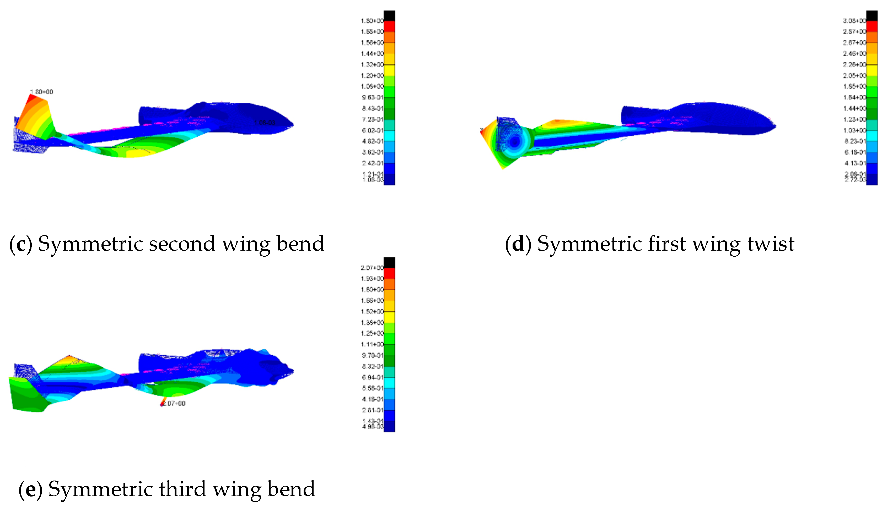
| Model Name | Pitching Mode | Symmetric First Wing Bend | Symmetric Wing Second Bend | Symmetric Wing First Twist | Symmetric Wing Third Bend |
|---|---|---|---|---|---|
| FEM | 0.0 | 5.19 | 24.55 | 47.16 | 62.18 |
| GVT | 0.0 | 5.10 | 23.60 | 44.17 | - |
| Error | 0.0% | 1.7% | 4.0% | 6.8% | - |
| Calculation or Experimental Status | Flutter Velocity (m/s) | Flutter Frequency (Hz) | Vibration Frequency and Damping under the Experimental Flutter Velocity | ||
|---|---|---|---|---|---|
| Frequency (Hz) | Damping (%) | ||||
| Benchmark status | Experiment | 22.3 | 1.67 | ||
| CFD/CSD | 19.21 | 1.31 | 1.47 | 7.7% | |
| Center of gravity moved forward 40 mm | Experiment | 24.2 | 2.73 | ||
| CFD/CSD | 19.77 | 1.88 | 2.62 | 10.8% | |
Publisher’s Note: MDPI stays neutral with regard to jurisdictional claims in published maps and institutional affiliations. |
© 2021 by the authors. Licensee MDPI, Basel, Switzerland. This article is an open access article distributed under the terms and conditions of the Creative Commons Attribution (CC BY) license (https://creativecommons.org/licenses/by/4.0/).
Share and Cite
Lei, P.; Guo, H.; LYu, B.; Chen, D.; Yu, L. Verification of a Body Freedom Flutter Numerical Simulation Method Based on Main Influence Parameters. Machines 2021, 9, 243. https://doi.org/10.3390/machines9100243
Lei P, Guo H, LYu B, Chen D, Yu L. Verification of a Body Freedom Flutter Numerical Simulation Method Based on Main Influence Parameters. Machines. 2021; 9(10):243. https://doi.org/10.3390/machines9100243
Chicago/Turabian StyleLei, Pengxuan, Hongtao Guo, Binbin LYu, Dehua Chen, and Li Yu. 2021. "Verification of a Body Freedom Flutter Numerical Simulation Method Based on Main Influence Parameters" Machines 9, no. 10: 243. https://doi.org/10.3390/machines9100243