Article

Key-Phase-Free Blade Tip-Timing for Nonstationary Test Conditions: An Improved Algorithm for the Vibration Monitoring of a SAFRAN Turbomachine from the Surveillance 9 International Conference Contest

1
Department of Mechanical and Aerospace Engineering, Politecnico di Torino, Corso Duca degli Abruzzi 24, 10129 Torino, Italy
2
College of Electrical Engineering and Automation, Anhui University, Hefei 230601, China
3
Laboratoire Vibrations Acoustique, INSA-Lyon, LVA EA677, F-69621 Villeurbanne, France
*
Author to whom correspondence should be addressed.
Machines 2021, 9(10), 235; https://doi.org/10.3390/machines9100235
Submission received: 20 September 2021 / Revised: 8 October 2021 / Accepted: 11 October 2021 / Published: 13 October 2021
(This article belongs to the Special Issue Feature Papers to Celebrate the First Impact Factor of Machines)

Abstract

:
A turbomachine is a fundamental engineering apparatus meant to transfer energy between a rotor and a fluid. Turbomachines are the core of power generation in many engineering applications such as electric power generation plants, aerospace, marine power, automotive etc. Their relevance makes them both mission critical and safety critical in many fields. To foster reliability and safety, then, continuous monitoring of the rotor is more than desirable. One promising monitoring technique is, with no doubt, the Blade Tip-Timing, which, being simple and non-invasive, can be easily implemented on many different rotors. Blade Tip-Timing is based on the recording of the time of arrival of the blades passing in front of a probe located at a fixed angular position. The non-contact nature of the measurement prevents influences on the measured vibration, that can be recovered for all the blades simultaneously, possibly even online. In this regard, a novel algorithm is presented in this paper for obtaining a good estimate of the vibration of the blades with minimum system complexity (i.e., only one Blade Tip-Timing probe) and minimum computational effort, so to create a simple vibration monitoring system, potentially implementable online. The methodology was tested on a dataset from a SAFRAN turbomachine made available during the Surveillance 9 international conference for a diagnostic contest.

1. Introduction

A turbomachine is a fundamental engineering apparatus meant to transfer energy between a rotor and a fluid. Turbomachines may either absorb energy to increase a fluid pressure, (i.e., pumps, fans, and compressors), or produce energy (i.e., turbines) by expanding a flow to lower pressures. Turbomachines are the core of power generation in many engineering applications such as electric power generation plants (i.e., hydro-electric turbines, steam turbines, gas turbines, windmills), aerospace (i.e., gas turbines in jet engines or turbopumps in rocket engines), marine power, automotive (turbochargers and superchargers), etc. Their relevance makes them mission critical as well as safety critical in many fields. To foster reliability and safety, then, continuous monitoring of the rotor, and in particular of the blades, is more than desirable. Traditionally, blade vibration was monitored by strain gauges installed on the blades [1,2,3]. Strain gauges are very precise contact sensors meant to measure strain. Nevertheless, they are impractical at many levels. In fact, each blade should be instrumented and wired, an operation that is difficult and could affect the blade vibration. Furthermore, the large centrifugal forces due to high rotational speeds may lead to a risk of sensor detachment and consequent projection, endangering operators and people nearby. In order to overcome these important shortcomings, a non-contact measurement technique dating back to the late 1960s [4,5,6] can be used. The technique took the name of Blade Tip-Timing (BTT) because it is based on the acquisition of the time at which a blade tip passes in front of a probe (i.e., a non-contact sensor such as a magnetic pick-up, an optical sensor, etc.) mounted on the casing. This timing is compared to a theoretical reference time (i.e., ideally, the passage of the non-vibrating root of the blade in front of another non-contact sensor in phase with the first) to produce an error that can be related to the blade tip vibration, assuming the knowledge of the instantaneous speed, which can be recovered from the blade roots probe signal (if the exact angle among the blades is known) or from an additional once-per revolution (OPR) sensor.
The first devices for BTT were proposed in the late 1960s/early 1970s and are reported in Figure 1. Such devices were analog and involved the measurement of the blade root passage time, which is, in general, a difficult task. Hence, with the advent of digital technology and computers, the typical Blade Tip-Timing system [7] turned out to be the one reported in Figure 2, involving an OPR probe and a tip-timing probe.
At least two critical considerations arise from the layout in Figure 2:
  • Under the assumption of constant rotational speed, with only one tip-timing sensor, the methodology is blind to synchronous vibration (i.e., integral order), as only asynchronous vibration can be effectively pictured [8];
  • A vibration response acquired at a single measurement location sampled at the rotation rate. A frequency spectrum will then feature aliasing for all the frequency components larger than half the rotation rate (i.e., the Nyquist limit) [8].
To face such issues, several modifications can be found in the literature. If it is true that it is possible to highlight synchronous resonances specifying nonstationary test conditions (i.e., by continuously varying the rotational speed in a range of interest) at the design level, this could be detrimental as the assembly under test could be damaged or destroyed by the resonance. On the contrary, multi-point measurements can give information on synchronous responses without having to pass the assembly through the peak value of the response. For example, at research level, systems with 50 or more probes were created. In any case, such a layout is very costly and never used at industrial level, where it is more likely to find a maximum of six probes [8,9,10]. As a matter of fact, the measurement system complexity and cost increases significantly with increases in the number of sensors, so that, in many cases, the OPR probe (i.e., the key phase sensor) is removed [11,12,13]. Finally, in order to solve the problem of sub-Nyquist BTT sampling rate, many signal reconstruction algorithms were proposed for recovering non-aliased spectra from the under-sampled signal and applied the algorithms both on simulated and experimental data [14,15,16,17,18].
The robustness of BTT algorithms with respect to the error in retrieving the blade tip vibration amplitude has recently gained interest, as a quantitative analysis can be very helpful in comparing different BTT schemes [13,19,20,21]. In particular, the main error sources in the BTT measurement chain are recognized to be:
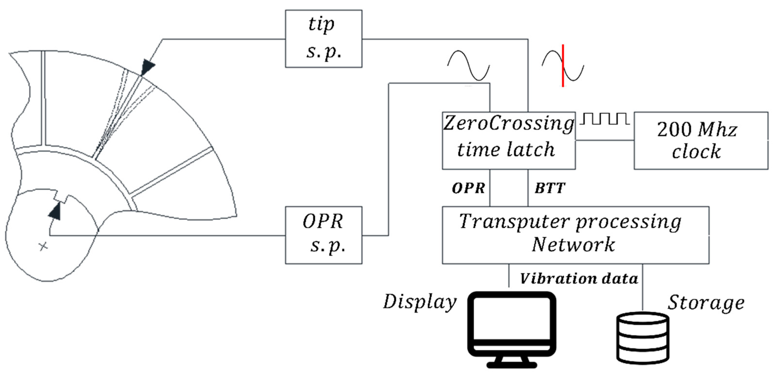
  • clock resolution (i.e., the time of arrival—ToA—of the blades are compared to an internal clock having a given resolution),
  • sensors vibration (i.e., the tip-timing and OPR probe are usually mounted on the casing, which vibrates during the turbomachine operation),
  • geometric errors of the blade mounting (i.e., the blades will never be perfectly equi-spaced),
  • non-stationarity (i.e., some algorithms assume uniform rotational speed, but speed fluctuations or fast accelerations may lead to additional error).
Of particular interest is the work in [13], where BTT is implemented on a large-scale industrial centrifugal compressor. Three important considerations arise. First, giving up the OPR sensor does not necessarily implies less accuracy; actually, for large scale turbomachinery where the OPR sensor is mounted on the shaft at a radial position which is way smaller than that of the tip-timing probe, the influence of casing vibration on the resulting blade vibration can be mitigated if an OPR-free method is used. Second, in the typical BTT method (i.e., with OPR sensor but no root probe) the error of the estimate of blade tip vibration is not uniform for all the blades but results in a larger error for the blades near the OPR. The error reduces as the blades get farther from the OPR. Third, BTT can be used for simple continuous monitoring of the health state of the blades if their vibration levels are compared. In fact, a damaged blade, having a reduced cross section, features different dynamic behavior with respect to a healthy one.
Starting from these considerations, the research challenge is that of proposing a novel diagnostic system for real-time online monitoring derived as an improvement to the algorithm in [13] (i.e., single probe tip timing, without root and OPR sensors), able to solve the issue of non-uniform error for the different blades, while featuring a reduced computational burden. The traditional and the novel improved BTT algorithm are described in the next section. Section 3 features a description of the Surveillance 9 contest test-rig and of the available dataset, while the results of the proposed BTT algorithm are shown in Section 4, where the non-stationary work conditions are also exploited to detect a synchronous resonance.

2. BTT Methodology: From the Traditional Algorithms to the Proposed Improvement

In this section, the traditional BTT methodology taken from [8] is summarized and compared to the OPR-free methodology in [13]. Finally, the proposed improvement is described.

2.1. Traditional BTT

The aim of BTT is that of recovering the blade vibration from the blade tips passage times (i.e., the ToA of the blades). If the tip displacement relative to the blade root is considered, this can be obtained as:
x ( t r o o t [ n ] ) = v ( t r o o t [ n ] ) · ( t t i p [ n ] t r o o t [ n ] )
where t r o o t is the root ToA (i.e., the so called “rotating datum”, a reference point on the blade assembly which does not vibrate) collecting the ideal passage times for all the blades (i.e., 1 to M, where M is the total number of blades) and revolution after revolution, t t i p is the tip ToA, v ( t r o o t ) = R t · ω ( t r o o t ) is the instantaneous tangential speed at tip radius R t , which is proportional to the angular speed ω , and x ( t r o o t ) is the finally obtained tangential displacement of the blade tip (i.e., the blade vibration).
If the rotating datum t r o o t can be measured directly (i.e., with a root probe aligned to the tip probe), the only information left is the instantaneous speed, which will be estimated from the root ToA or from the OPR ToA as
v ( t r o o t [ n ] ) = R t · Δ α Δ t r o o t [ n ]
where Δ t r o o t [ n ] = t r o o t [ n + 1 ] t r o o t [ n ] is the time taken for the rotor to make a rotation of Δ α radians. Notice that if the OPR sensor is used, Δ α = 2 π and t r o o t becomes t o p r (i.e., arrival time of the OPR).
Nevertheless, as already introduced in Section 1, the root probe is often difficult to install. Sometimes it can be substituted by an additional reference rotor on the shaft, as in Figure 1b, but in most of cases the sensor is given up. Hence, the BTT system ends up relying on tip-timings and OPR passage times, so that the rotating datum must be recovered from the OPR ToA. Under the assumption of M equispaced blades and uniform rotational speed, if the OPR sensor is assumed shifted backwards from the BTT sensor of an angle of 2 π / M radians, the rotating datum for the m-th blade (counted from the OPR sensor position) at the j-th revolution can be obtained as:
t ^ r o o t ( j , m ) = t o p r [ j ] + ( m M · ( t o p r [ j + 1 ] t o p r [ j ] ) ) = t ^ r o o t [ m + j · M ]
Hence, the blade datum times (i.e., t ^ r o o t ) are updated once per revolution so that errors are introduced when the rotor velocity varies within the revolution. These errors can be reduced using more expensive systems featuring multiple OPR probes to update the datum times at various points in a single revolution. In fact, in most practical applications, the tendency is to limit the number of probes as much as possible, so that OPR-free algorithms were proposed.
In [8], for example, a method based on tip-time averaging is reported (i.e., Blade Tip Time Averaging—Ives (1986)), but few information can be found. The idea seems to be that of using a running average on the ToA of a given blade, so as to directly reconstruct the rotating datum of the blade, without the need of passing through the OPR signal. This translates into a sort of moving synchronous average formulation, which for an even length R of the window corresponds to:
t ^ r o o t ( a ) [ n ] = 1 R + 1 r = R / 2 R / 2 t t i p [ n + r · M ]
According to [8] then, the worst error in the t ^ r o o t ( a ) [ n ] approximation occurs when the blade response amplitude remains constant at the measurement point on successive assembly rotations. In this case the datum and tip passing times are identical and the calculated displacement is zero. Additionally, some fluctuations may not be well removed by the averaging algorithm, whose performance depends on the length R of the averaging.
In [13], on the contrary, the OPR ToA are reconstructed from the tip-timing signal as the average of the ToA of all the blades in two following rotations (i.e., j-th and j+1-th rotations):
t ^ o p r [ j ] = 1 2 M n j t h   ( j + 1 ) t h t t i p [ n ]
The so obtained t ^ o p r are then used in a formula similar to Equation (3), that considers the actual spacing of the blades instead of the ideal m / M , valid only for perfectly equi-spaced blades.
The substitution of root timing or OPR timing with an average of the measurements of the vibrating tips of the M blades may sound inaccurate, and has its accuracy limit. Nevertheless, the analysis in [13] proved that such a methodology is more robust to additional error sources such as sensors vibration, in particular when the OPR or root probes are placed at smaller radial positions than the tip probes. As a matter of fact, the application of such an algorithm to the large-scale centrifugal compressor in [13] led to better results than using an OPR sensor on the shaft.
The idea of this work is then to combine the intentions of two finally introduced approaches to get an improved OPR-free methodology. This is described in the next section.

2.2. The Proposed Improvement

The proposed improvement comes after three considerations:
  • the OPR and root sensors-free approach in [13] is based on the reconstruction of the OPR signal and has then a non-uniform error in the estimate of the vibration of the different blades. This is mathematically proven in [13], by analyzing the error propagation of the final formula derived by Equations (1)–(3). In fact, as established in [13], the reconstructed vibration for the m-th blade at j-th cycle in angular fraction a-dimensional units (i.e., blade displacement divided by 2 π R t ), can be written as:
    x ( t t i p [ m + j · M ] ) 2 π R t = t t i p [ m + j · M ] t ^   o p r [ j ] t ^ o p r [ j + 1 ] t ^ o p r [ j ] c m
    where t ^ o p r [ j ] is estimated with Equation (5), and c m is the theoretical angular ratio of the m-th blade (i.e., a constant equal to m / M , as in Equation (3), if the assumption of perfectly spaced blades holds, and the reconstructed OPR position corresponds to the M-1-th blade position), which can be substituted by the true angular ratio when available (N.B., commonly an estimation of such a geometrical error is done to characterize the rotor under analysis in a sort of calibration procedure). In [13] it is proved that such a formulation leads to a parabolic trend for the squared vibration error (i.e., maximum error for the blades m = 1 and m = M near the OPR position, and minimum for the mid-blades m ~ M / 2 ), effect which is undesirable as may act as a confounding influence in a diagnostic system.
  • in [8] it is said that the error in the standard OPR based methodology can be reduced if multiple OPR probes are used to update the datum times at various points in a single revolution.
  • the OPR and root sensors-free approach in [8] (i.e., Blade Tip Time Averaging—Ives (1986)), is presumed to be based on the reconstruction of the root signal of a blade at a given rotation as the average of the tip timings of that blade in adjacent rotations (Equation (4)). This had the advantage of a direct vibration estimation bypassing the OPR signal reconstruction and the geometric error issue (i.e., the calibration of the c m for the different blades is not needed). The drawback is that, in non-stationary conditions, the average cannot involve too many cycles, otherwise the stationarity assumption will not hold anymore. On the contrary, in stationary conditions, if synchronous vibration is predominant, a vibrating blade could deflect of the same amount in following cycles when passing the BTT sensor, leading to an erroneous zero vibration value.
The idea of this work is then to combine the two reference methodologies so to derive a BTT scheme similar to that in [13], but with a uniform error for the vibration estimate of the different blades, following the multi OPR advice in [8]. This can be obtained if Equation (5) is modified to get a different OPR signal for each blade (i.e., as if M-OPR sensors placed between the blades were used). That is, if the cycle after cycle iteration is simplified into a continuous moving window, the estimate is no more a function of the cycle but of the sample. Hence, the OPR estimate in [13] (function of the j-th cycle, see Equation (5)) is substituted by a novel (yet biased) estimate of t r o o t (i.e., the rotating datum), which is function of the n-th sample:
t ^ r o o t ( b ) [ n ] = 1 2 M r = M M 1 t t i p [ n + r ]
and can be updated sample after sample. It should be noticed that Equation (7) results similar to Equation (4) but is actually simpler as corresponds to a moving average of the BTT signal. Using Equation (7), the final vibration estimate is biased by a quantity near to half the geometric spacing between the blades 1 2 M = c m t h e o r e t i c a l . In fact, it can be written:
x ( t t i p [ n ] ) 2 π R t + c n     n / M   =   t t i p [ n ]     t ^ r o o t ( b ) [ n ] t ^ r o o t ( b ) [ n + M ]     t ^ r o o t ( b ) [ n ] =   2 M · t t i p [ n ]     r   =     M M     1 t t i p [ n + r ] r   =   M 2 M     1 t t i p [ n + r ]     r   =     M     1 t t i p [ n + r ]
where n / M is the floor function, giving the greatest integer less than or equal to n / M , while the estimate of the rotational period is obtained as:
t ^ r o o t ( b ) [ n + M ] t ^ r o o t ( b ) [ n ] = 1 / f ^ ( b ) [ n ] = T ^ ( b ) [ n ]
Notice that the left-hand side term in Equation (8) is a biased estimate of the blades’ vibration in angular fraction a-dimensional units. By removing a proper estimate of c m (N.B., one per each different blade to compensate for geometrical mistuning) and multiplying by 2 π R t , the true vibration as tip displacement relative to the blade root can be obtained. Finally, the signals for the vibration of the different blades at each revolution j can be obtained as
x m [ j ] = x ( t t i p [ m + j · M ] )
The here proposed improved algorithm will be compared to the reference algorithms in [13,8] (i.e., the presumed algorithm of Blade Tip Time Averaging—Ives (1986), which was impossible for the authors to find) on the dataset from the Surveillance 9 contest, described in the next section.

3. Surveillance 9 Contest Test-Rig and Data Description

The system that will be analyzed in this paper is the SAFRAN turbine, object of the contest of the Surveillance 9 international conference held in Fez, Morocco on the 22–24 March 2017. Three optical sensors for tip-timing were mounted on the casing. Each sensor triggers when a blade passes in front of it and the time instants of each blade passing event (i.e., the ToA) are stored into three vectors (one per sensor), that constitute the data provided for the contest. No additional information was further given, so that the actual configuration should be recovered from the data itself. In particular, it was required to retrieve:
  • the number of blades;
  • the precise angles between each pair of consecutive blades (noting blade # 1, 2, 3 … the first, second, third… blade passing in front of sensor 1);
  • which blade is passing first on sensors 2 and 3;
  • the direction of rotation (a blade is passing successively over sensor 1, 2, 3 or 1, 3, 2);
  • the angular position of sensors 2 and 3, assuming sensor 1 is at 0 degree, with a rotation direction defined by the rotation of the turbine.
In this section, a way to obtain such a relevant information for defining the system layout is given. All the considerations here reported exploit the uneven spacing of following blades of real turbines (i.e., the geometric error).

3.1. Number of Blades

As previously stated, real turbines always feature unequal spacing of the blades. Hence, in stationary conditions, the time difference between following blades will vary in a cycle repeating revolution after revolution. In order to highlight such a hidden periodicity, the autocorrelation could be employed. In this particular case, as no information was given about the rotational speed, in order to fulfill the stationarity assumption, a sort of short-time autocorrelation is adopted. As a matter of fact, if a window of few samples (i.e., a number larger than the number of blades M, but not too large to limit the acceleration/deceleration effect—e.g., 100 in this case) is selected, the speed variability will be limited, and the autocorrelation will remain meaningful. Considering no overlap and averaging the autocorrelations for all the following windows, the pattern in Figure 3 is highlighted. As it is easy to see, a periodicity of 11 samples is present, indicating a number of blades M = 11 .

3.2. Precise Angle between Consecutive Blades

In order to estimate the angle between consecutive blades, the difference signal of the ToA will be exploited again. In fact, in stationary conditions (hypothesis assumed to hold during a single revolution), the ratio of time-difference over rotation period equals the angular fraction of spaced angle:
t t i p [ n + 1 ] t t i p [ n ] T = Δ α 2 π
Thus, if an estimate of the period T ^ (or of the rotational frequency f ^ = 1 / T ^ ) is used, an estimate of the angular fraction can be obtained. As in Section 3.1, the actual number of blades was computed (i.e., M = 11 ), the simplest estimate of the period can be:
T ^ = t t i p [ n + M ] t t i p [ n ]
Clearly, the accuracy in the time ratio will be affected by the blade vibration, but if the procedure is repeated cycle after cycle, many estimates can be obtained. Averaging the angular ratio blade by blade, the result of the estimation for the three probes is reported in the following table.
It is important to remember that the blade which passes first in front of the first sensor, will only later reach the other sensors, so that a rephasing is necessary. If the estimates in Table 1 are put into a graph, such a rephasing can be done even by eye, without the need of mathematical artifacts such as the cross-correlation. The repeating pattern in the three plots in Figure 4 is indeed evident.
Focusing on the minimum, for example, this occurs at sample 1–2 for probe 1, at sample 9–10 for probe 2, and at sample 8–9 for probe 3. Hence, if the blade numbering is done on the first probe signal, naming blade 1 the first passing in front of the sensor, blade 2 the second, etc., the x axis of the first probe directly corresponds to a blade axis, while the x axes of the second and third probes should be corrected so that blades 1–2 will correspond to samples 9–10 and samples 8–9, respectively. Hence, Table 1 can be easily modified into Table 2. This will help to understand both of the next two questions that will be answered in the next section: which blade is passing first on sensors 2 and 3 and which is the direction of rotation (a blade is passing successively over sensor 1, 2, 3 or 1, 3, 2).

3.3. First Blade in Front of the Different Sensors and Direction of Rotation

Once the blade standard names are given, and Table 2 is produced visually exploiting the cross correlation among the three signals in Figure 4, it is easy to retrieve further piece of information from the data. In particular, it is easy to read from Table 2 that, being blade 1 the first passing in front of probe 1, and blade 2 the second passing in front of probe 1, etc., the first blade passing in front of probe 2 is blade 4, while the first passing in front of probe 3 is blade 5. From this consideration is then easy to draw a scheme of the setup of the BTT system. This is reported in Figure 5, where a clockwise rotation is assumed for the turbine. The probes are also added in the only possible way coherent with the considerations arisen in this section.
Hence, a rotating blade will be recorded by sensor 1 first, then by sensor 3 and as last, by sensor 2 during a complete cycle (i.e., sensors are seen in the order 1, 3, 2 from a rotating blade).

3.4. Angular Position of Sensors 2 & 3 with Respect to Sensor 1
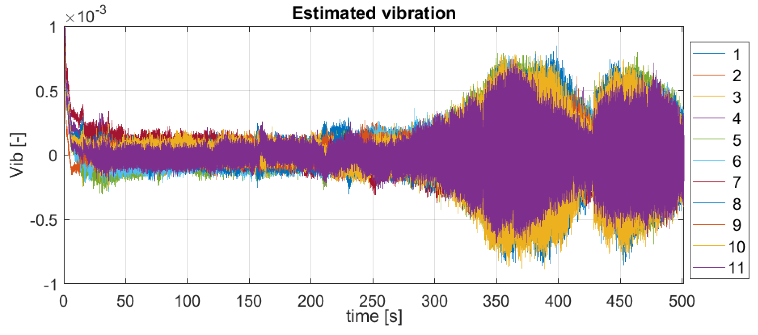
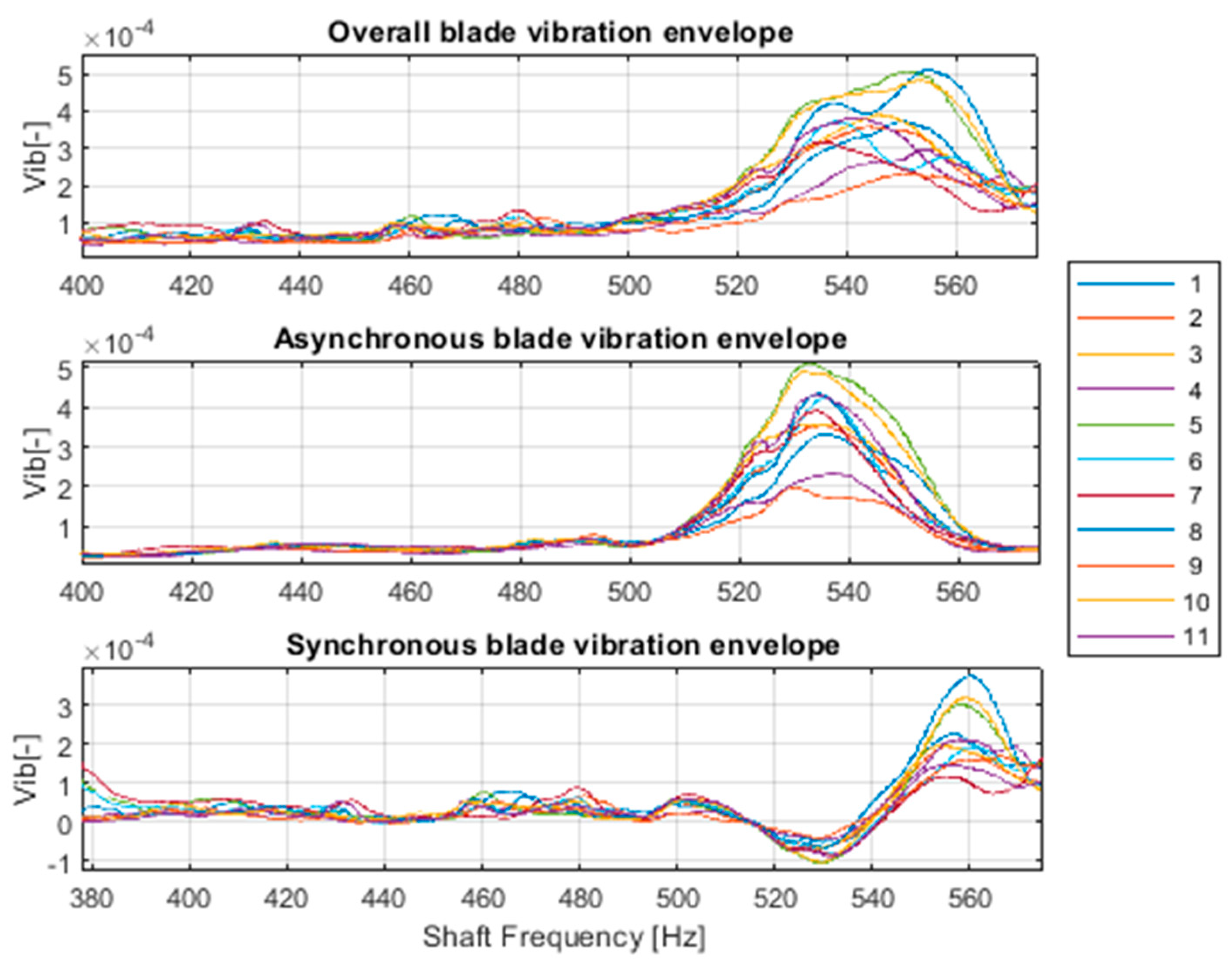
From the scheme in Figure 5, it is clear that sensor 3 is roughly located at an angular fraction of at least 7 / 11 if sensor 1 is considered as the reference and the angle is measured along the direction of rotation (i.e., the precise position will be for sure more than 229° with respect to sensor 1), while sensor 2 is further away, at a minimum angular fraction of 8 / 11 (i.e., at least at 262.8° from sensor 1). In order to get a better estimate, a procedure similar to that used for the precise estimation of the angle between following blades can be used.
In particular, blade 1 passes in front of sensor 1 at t t i p 1 [ 1 ] (i.e., the first sample measured by probe 1-N.B., the apex is used to indicate the sensor number), and then reaches sensor 3 at t t i p 3 [ 8 ] , and sensor 2 at t t i p 2 [ 9 ] . Under the assumption of stationarity during a cycle, equation 9 holds, so that it is possible to estimate the angular position of the sensors with respect to sensor 1 as an average along the total number of cycles n c :
α 3 = 1 n c j 360 · t t i p 3 [ j + 7 ] t t i p 1 [ j ] t t i p 1 [ j + M ] t t i p 1 [ j ] α 2 = 1 n c j 360 · t t i p 2 [ j + 8 ] t t i p 1 [ j ] t t i p 1 [ j + M ] t t i p 1 [ j ]
The so obtained precise estimates are α 2 = 263.9 °   ±   0.1 ° and α 3 = 240.0 °   ±   0.1 ° , so that the BTT system setup is now completely defined.

4. Results

In this section, the algorithm proposed in Section 2.2. is applied to the signal of the first probe of the dataset from Surveillance 9 contest and compared to the results obtained using the reference methodology described in [13] and in [8] (the presumed algorithm of Blade Tip Time Averaging—Ives (1986)).
As first, the raw ToA are shown in Figure 6. The raw ToA are then processed with Equation (7), a simple moving average, from which an estimate of the rotational speed (Figure 7) can be obtained using Equation (9). Finally, Equations (8) and (10) are applied to obtain a-dimensional biased estimates of the blade vibration (i.e., as angular fraction). The bias is due to the presence of the term c n [ n / M ] in Equation (8). This bias can be compensated by removing the average vibration level. In fact, not having the true calibration information, the average of the vibration signal is the better estimate. The result is shown in Figure 8.
If the vibration of the first blade is considered, a comparison can be done with respect to the two reference methods. As can be seen in Figure 9, the proposed improved method leads to results which are not far from [8,13]. In particular, focusing on the time domain, the signal is practically the same of that obtained from the method in [8], apart from a different amplitude modulation. Nevertheless, the same vibration envelope of method [13] is obtained. The difference in the envelope obtained with method [8] can be attributed to the previously highlighted drawback, being such a method blind to synchronous vibration. The proposed method puts then together the algorithm efficiency of method [8] with the ability of method [13] which is sensitive both to synchronous and asynchronous blade vibration. Indeed, focusing on the computational times, on the same PC (i.e., intel i7-7700 CPU @ 3.6 GHz and 32 GB of RAM), the proposed algorithm proves to be the fastest, as highlighted in Table 3. This occurs because method [13] is based on Equations (5) and (6) which, without the considerations in this paper, was implemented via two for-loops cycling through the whole signal length (i.e., of the order 2.5 × 10 6 samples). However, if Equation (5) is modified to get a different OPR signal for each blade, the cycle after cycle iteration can be simplified into a continuous moving average of the BTT signal (Equations (7) and (8)), and the algorithm can be implemented with a single convolution, which is much more computationally efficient and can be easily optimized for on-line monitoring.
In order to highlight synchronous resonances, the nonstationary test conditions (i.e., the frequency sweep from 400 to 570 Hz visible in Figure 7) are exploited. Plotting the vibration envelope against the rotational frequency, a sort of amplitude spectrum can be obtained, as shown in Figure 10, where the results of the proposed method and of the method in [8] are subtracted to finally highlight the synchronous contribution.
It is interesting to notice that both an asynchronous and a synchronous resonance appear at about 530 Hz and 560 Hz, respectively. Furthermore, not all the blades share the same dynamic response. In particular, blades #5, #8 and #10 feature lower overall vibration levels, while blades #7 and #11 experience larger vibration.
Finding an explanation for such synchronous and asynchronous contributions is out of the scope of this work. In general, asynchronous vibration usually occurs in case of abnormal conditions, such as rotating stall, surge, flutter, and bearing vibration. In these cases, the blade vibration frequency is a non-integer multiple of the rotating frequency and the phase of the response can be arbitrary [22]. Synchronous vibration, on the contrary, is excited by the multiples of the rotating frequency. It is associated with the bladed assemblies and is affected by blade geometry, coupling, mistuning, airflow etc. [23].

5. Conclusions

In this paper, the OPR-free BTT methodology introduced in [13] is improved so to produce a uniform error in the estimated blade vibration. The modified methodology is based on the direct reconstruction of the rotating datum (i.e., the root ToA) instead of the reconstruction of the OPR signal. This not only flattens the parabolic trend of the squared vibration error in [13] but makes the computation order of magnitude faster as well. The proposed methodology is similar to that described in [8] (Blade Tip-Time Averaging—Ives (1986)) but is actually superior as it uses the ToA of all the blades for reconstructing a rotating datum, so that it results sensitive to synchronous vibration too. In this regard, a synchronous resonance was highlighted in this paper exploiting both the methods and taking advantage of the non-stationary work conditions.
To conclude, the here proposed improved methodology fosters the on-line condition monitoring of turbomachines and could be used for diagnostic purposes if an anomaly detection (e.g., [24,25,26,27,28,29,30]) is conducted on the vibration signal of the different blades.
Further works may involve a quantitative error analysis of the here proposed algorithm with respect to a true reference vibration (e.g., acquired with the more complex strain gauge measurement system) and the evaluation of the effects of possible modifications to the algorithm. Indeed, as Equation (7) corresponds to a simple moving average of order 2 M , it could be reasonable to investigate the behavior of the algorithm with different orders or by implementing a weighted moving average or different Finite Impulse Response filters.

Author Contributions

Conceptualization, A.P.D.; methodology, A.P.D., C.H.; software, A.P.D.; validation, A.P.D., L.G. and J.A.; formal analysis, A.P.D.; investigation, A.P.D.; resources, A.P.D. and L.G.; data curation, A.P.D.; writing—original draft preparation, A.P.D.; writing—review and editing, A.P.D.; visualization, A.P.D.; supervision, L.G. and J.A.; project administration, L.G.; All authors have read and agreed to the published version of the manuscript.

Funding

This research received no external funding.

Institutional Review Board Statement

Not applicable.

Informed Consent Statement

Not applicable.

Data Availability Statement

The dataset was downloaded online during the international conference Surveillance 9 (Fez, Morocco, 22–24 March 2017) at https://surveillance9.sciencesconf.org/resource/page/id/13.html (accessed on 10 October 2021).

Acknowledgments

We thank the Surveillance 9 organizing committee (Simon BRAUN, Jérôme ANTONI and Luigi GARIBALDI), and in particular the contest organizers Quentin LECLER and Hugo ANDRE as well as SAFRAN for the making the dataset available.

Conflicts of Interest

The authors declare no conflict of interest.

List of Symbols and Abbreviations

BTTBlade Tip Timing
ToATime of Arrival
OPROnce Per Revolution
M Number of blades
m Blade index
j Cycle index
n Sample   index   ( n = m + j   · M )
n c Total number of cycles
t t i p [ n ] Tip ToA
t r o o t [ n ] Root ToA
t o p r [ j ] OPR ToA
R t Tip radius
f ( t ) Shaft frequency
ω ( t ) = 2 π f ( t ) Instantaneous shaft angular speed
T ( t ) = 1 f ( t ) Instantaneous period of the shaft rotation

References

  1. Prochazka, P.; Vanek, F. New Methods of Noncontact Sensing of Blade Vibrations and Deflections in Turbomachinery. IEEE Trans. Instrum. Meas. 2013, 63, 1583–1592. [Google Scholar] [CrossRef]
  2. Battiato, G.; Firrone, C.M.; Berruti, T. Forced response of rotating bladed disks: Blade Tip-Timing measurements. Mech. Syst. Signal Process. 2017, 85, 912–926. [Google Scholar] [CrossRef]
  3. Wang, Z.K.; Yang, Z.B.; Wu, S.M.; Li, H.Q.; Tian, S.H.; Chen, X.F. An improved multiple signal classification for non-uniform sampling in blade tip timing. IEEE Trans. Instrum. Meas. 2020, 69, 7941–7952. [Google Scholar] [CrossRef]
  4. Heath, S.; Imregun, M. A Survey of Blade Tip-Timing Measurement Techniques for Turbomachinery Vibration. J. Eng. Gas Turbines Power 1998, 120, 784–791. [Google Scholar] [CrossRef]
  5. Zablotskiy, I.Y.; Korostelev, Y.A. Measurement of Resonance Vibrations of Turbine Blades with the Elura Device. Energomashi-Nostroneniye 1970, 36–39. [Google Scholar]
  6. Hohenberg, R. Detection and study of compressor-blade vibration. Exp. Mech. 1967, 7, 19A–24A. [Google Scholar] [CrossRef]
  7. Heath, S.; Imregun, M. An improved single-parameter tip-timing method for turbomachinery blade vibration measurements using optical laser probes. Int. J. Mech. Sci. 1996, 38, 1047–1058. [Google Scholar] [CrossRef]
  8. Heat, S. A Study of Tip-Timing Measurement Techniques for the Determination of Bladed-Disk Vibration Characteristics. Ph.D. Thesis, Imperial College, London, UK, 1997. [Google Scholar]
  9. Carrington, I.B.; Wright, J.R.; Cooper, J.; Dimitriadis, G. A comparison of blade tip timing data analysis methods. Proc. Inst. Mech. Eng. Part G: J. Aerosp. Eng. 2001, 215, 301–312. [Google Scholar] [CrossRef]
  10. Wang, W.; Ren, S.; Huang, S.; Li, Q.; Chen, K. New Step to Improve the Accuracy of Blade Synchronous Vibration Parameters Identification Based on Combination of GARIV and LM Algorithm. In Proceedings of the ASME Turbo Expo 2017: Turbomachinery Technical Conference and Exposition, American Society of Mechanical Engineers, Charlotte, NC, USA, 26–30 June 2017. [Google Scholar] [CrossRef]
  11. Guo, H.; Duan, F.; Zhang, J. Blade resonance parameter identification based on tip-timing method without the once-per revolution sensor. Mech. Syst. Signal Process. 2016, 66-67, 625–639. [Google Scholar] [CrossRef]
  12. Wang, Z.K.; Yang, Z.B.; Wu, S.M.; Li, H.Q.; Yan, R.Q.; Tian, S.H.; Zhang, X.W.; Chen, X.F. An OPR-free blade tip timing method based on blade spacing change. In Proceedings of the IEEE International Instrumentation and Measurement Technology Conference (I2MTC), Ottawa, ON, Canada, 16–19 May 2020. [Google Scholar]
  13. He, C.; Antoni, J.; Daga, A.P.; Li, H.; Chu, N.; Lu, S.; Li, Z. An Improved Key-Phase-Free Blade Tip-Timing Technique for Nonstationary Test Conditions and Its Application on Large-Scale Centrifugal Compressor Blades. IEEE Trans. Instrum. Meas. 2020, 70, 1–16. [Google Scholar] [CrossRef]
  14. Wu, S.; Zhao, Z.; Yang, Z.; Tian, S.; Yang, L.; Chen, X. Physical constraints fused equiangular tight frame method for Blade Tip Timing sensor arrangement. Measurement 2019, 145, 841–851. [Google Scholar] [CrossRef]
  15. Hu, Z.; Lin, J.; Chen, Z.-S.; Yang, Y.-M.; Li, X.-J. A Non-Uniformly Under-Sampled Blade Tip-Timing Signal Reconstruction Method for Blade Vibration Monitoring. Sensors 2015, 15, 2419–2437. [Google Scholar] [CrossRef] [Green Version]
  16. Lin, J.; Hu, Z.; Chen, Z.-S.; Yang, Y.-M.; Xu, H.-L. Sparse reconstruction of blade tip-timing signals for multi-mode blade vibration monitoring. Mech. Syst. Signal Process. 2016, 81, 250–258. [Google Scholar] [CrossRef]
  17. Pan, M.; Yang, Y.; Guan, F.; Hu, H.; Xu, H. Sparse Representation Based Frequency Detection and Uncertainty Reduction in Blade Tip Timing Measurement for Multi-Mode Blade Vibration Monitoring. Sensors 2017, 17, 1745. [Google Scholar] [CrossRef] [PubMed] [Green Version]
  18. Wu, S.; Russhard, P.; Yan, R.; Tian, S.; Wang, S.; Zhao, Z.; Chen, X. An Adaptive Online Blade Health Monitoring Method: From Raw Data to Parameters Identification. IEEE Trans. Instrum. Meas. 2020, 69, 2581–2592. [Google Scholar] [CrossRef]
  19. Salhi, B.; Lardiès, J.; Berthillier, M.; Voinis, P.; Bodel, C. Modal parameter identification of mistuned bladed disks using tip timing data. J. Sound Vib. 2008, 314, 885–906. [Google Scholar] [CrossRef]
  20. Rossi, G.; Brouckaert, J.F. Design of blade tip timing measurements systems based on uncertainty analysis. In Proceedings of the 58th International Instrumentation Symposium, San Diego, CA, USA, 4–8 June 2020; pp. 4–8. [Google Scholar]
  21. Ren, S.; Xiang, X.; Zhao, W.; Zhao, Q.; Wang, C.; Xu, Q. An error correction blade tip-timing method to improve the measured accuracy of blade vibration displacement during unstable rotation speed. Mech. Syst. Signal Process. 2021, 162, 108030. [Google Scholar] [CrossRef]
  22. Liu, Z.; Duan, F.; Niu, G.; Ma, L.; Jiang, J.; Fu, X. An Improved Circumferential Fourier Fit (CFF) Method for Blade Tip Timing Measurements. Appl. Sci. 2020, 10, 3675. [Google Scholar] [CrossRef]
  23. Dimitriadis, G.; Carrington, I.; Wright, J.; Cooper, J. Blade-tip timing measurement of synchronous vibrations of rotating bladed assemblies. Mech. Syst. Signal Process. 2002, 16, 599–622. [Google Scholar] [CrossRef]
  24. Daga, A.P.; Garibaldi, L. Machine Vibration Monitoring for Diagnostics through Hypothesis Testing. Information 2019, 10, 204. [Google Scholar] [CrossRef] [Green Version]
  25. Daga, A.P.; Fasana, A.; Marchesiello, S.; Garibaldi, L. The Politecnico di Torino rolling bearing test rig: Description and analysis of open access data. Mech. Syst. Signal Process. 2018, 120, 252–273. [Google Scholar] [CrossRef]
  26. Castellani, F.; Garibaldi, L.; Daga, A.P.; Astolfi, D.; Natili, F. Diagnosis of Faulty Wind Turbine Bearings Using Tower Vibration Measurements. Energies 2020, 13, 1474. [Google Scholar] [CrossRef] [Green Version]
  27. Daga, A.P.; Fasana, A.; Garibaldi, L.; Marchesiello, S. Big Data management: A Vibration Monitoring point of view. In Proceedings of the 2020 IEEE International Workshop on Metrology for Industry 4.0 & IoT, Rome, Italy, 3–5 June 2020; pp. 548–553. [Google Scholar]
  28. Natili, F.; Daga, A.P.; Castellani, F.; Garibaldi, L. Multi-Scale Wind Turbine Bearings Supervision Methods Using Industrial SCADA and Vibration Data. Appl. Sci. 2021, 11, 6785. [Google Scholar] [CrossRef]
  29. Daga, A.P.; Garibaldi, L.; Bonmassar, L. Turbomolecular high-vacuum pump bearings diagnostics using temperature and vibration measurements. In Proceedings of the IEEE International Workshop on Metrology for Industry, Rome, Italy, 7–9 June 2021; pp. 264–269. [Google Scholar] [CrossRef]
  30. Gao, Z.; Liu, X. An Overview on Fault Diagnosis, Prognosis and Resilient Control for Wind Turbine Systems. Processes 2021, 9, 300. [Google Scholar] [CrossRef]
Figure 1. Reproduction of early BTT devices: (a) the USSR ELURA analogue device (1970) [5], (b) the Avco-Lycoming device (1967) [6].
Machines 09 00235 g001
Figure 2. Reproduction of a typical blade tip-timing system (1996) [7].
Machines 09 00235 g002
Figure 3. Average of short-time autocorrelations on difference signal–window: 100 samples, overlap: 0 samples. N.B., just the first 50 positive shifts are shown.
Machines 09 00235 g003
Figure 4. Precise angle (°) between consecutive samples estimated from the three different signals.
Machines 09 00235 g004
Figure 5. Schematic setup of the BTT system retrieved from the available data acquired from the three probes (optical sensors), assuming a clockwise turbine rotation.
Machines 09 00235 g005
Figure 6. ToA of the probe 1 for the BTT system of the Surveillance 9 contest (see Section 3).
Machines 09 00235 g006
Figure 7. Estimate of the rotational frequency from the moving averaged ToA (Equation (9)).
Machines 09 00235 g007
Figure 8. Estimate of the blade vibration with the proposed algorithm (in angular fraction adimensional units, see Equation (12)) for all the 11 blades—see Equation (8).
Machines 09 00235 g008
Figure 9. (a) Comparison of the blade #1 adimensional vibration estimated with the proposed algorithm and of the estimates obtained by the reference methodology in [8,13] (Blade Tip Time Averaging—Ives (1986)) with a zoom (b). A smoothed vibration envelope is reported in (c).
Machines 09 00235 g009
Figure 10. Synchronous and asynchronous vibration amplitude (adimensional) as a function of the rotational frequency of the shaft for all the 11 blades.
Machines 09 00235 g010
Table 1. Precise angle (°) between consecutive samples estimated from the three different probes. The minimum estimate accuracy is ±   0.07 °. The ideal would be 360 ° / M = 32.727 °.
Samp1–22–33–44–55–66–77–88–99–1010–1111–1
Probe132.5032.9032.7432.7232.7232.7832.5832.7832.8232.7132.74
Probe232.6932.7232.8232.5332.7932.8532.6832.7632.4632.9332.76
Probe332.7332.8232.5632.7832.8332.6932.7532.4632.9432.7232.73
Table 2. Precise angle (°) between consecutive blades estimated from the three different probes. The minimum estimate accuracy is ± 0.07 °. The ideal would be 360 ° / M = 32.727 °.
Blades1–22–33–44–55–66–77–88–99–1010–1111–1
Probe132.5032.9032.7432.7232.7232.7832.5832.7832.8232.7132.74
Blades4–55–66–77–88–99–1010–1111–11–22–33–4
Probe232.6932.7232.8232.5332.7932.8532.6832.7632.4632.9332.76
Blades5–66–77–88–99–1010–1111–11–22–33–44–5
Probe332.7332.8232.5632.7832.8332.6932.7532.4632.9432.7232.73
Table 3. Computational times (average over three runs) for the different algorithms on a 3.6 GHz CPU and 32 GB RAM machine.
Algorithmt [s]
Ref. [13]141.7
Ref. [8]0.09
Proposed0.04
Publisher’s Note: MDPI stays neutral with regard to jurisdictional claims in published maps and institutional affiliations.

