Article

A Data-Driven Framework for Early-Stage Fatigue Damage Detection in Aluminum Alloys Using Ultrasonic Sensors

by
Susheel Dharmadhikari
1,
Chandrachur Bhattacharya
1,
Asok Ray
1,2 and
Amrita Basak
1,*
1
Department of Mechanical Engineering, The Pennsylvania State University, University Park, PA 16802, USA
2
Department of Mathematics, The Pennsylvania State University, University Park, PA 16802, USA
*
Author to whom correspondence should be addressed.
Machines 2021, 9(10), 211; https://doi.org/10.3390/machines9100211
Submission received: 2 August 2021 / Revised: 15 September 2021 / Accepted: 16 September 2021 / Published: 25 September 2021
(This article belongs to the Special Issue Feature Papers to Celebrate the First Impact Factor of Machines)

Abstract

:
The paper presents a coupled machine learning and pattern recognition algorithm to enable early-stage fatigue damage detection in aerospace-grade aluminum alloys. U- and V-notched Al7075-T6 specimens are instrumented with a pair of ultrasonic sensors and, thereafter, tested on an MTS apparatus integrated with a confocal microscope and a digital microscope. The confocal microscope is focused on the notch root of the specimens, whereas the digital microscope is focused on the side of the notch. Two features, viz., the crack opening displacement (COD) and the crack length, are extracted during the tests in addition to the ultrasonic signal data. These signal data are analyzed using a machine learning framework that is built upon a symbolic time-series algorithm. This framework is interrogated for crack detection in the crack coalescence (CC) regime defined by COD of ~3 μm and detected through the confocal microscope. Additionally, the framework is probed in the crack propagation (CP) regime characterized by a crack length of ~0.2 mm and detected via the digital microscope. For the CC regime, training accuracies of 79.82% and 81.94% are achieved, whereas testing accuracies of 68.18% and 74.12% are observed for the U- and V-notched specimens, respectively. For the CP regime, overall training accuracies of 88.3% and 91.85% are observed, and accordingly, testing accuracies of 81.94% and 85.62% are obtained for the U- and V-notched specimens, respectively. The results show that a combined machine learning and pattern recognition algorithm enables robust and reliable fatigue damage detection in aerospace structural components.

1. Introduction

High-strength aluminum alloys such as Al2024, Al6061, and Al7075 are widely used in the fabrication of critical structural parts of aircraft components encompassing fuselage, fittings, gears, shafts, valves, etc. The critical failure mode of such structural components is often due to repetitive loadings, i.e., fatigue. Fatigue failures are challenging to predict and control due to their occurrence at seemingly safe loads where the structure operates well below the yield strength or the ultimate tensile strength of the material [1]. The mechanisms behind such failures are attributed to the cumulative accumulation of damage that leads to fatigue crack initiation and then eventually to fracture. The enigmatic characteristics of the fatigue failure phenomenon have garnered a significant amount of interest from the industry and academia alike [1]. Due to the impact of uncertain operating conditions, several parameters play critical roles in affecting the fatigue lives of aerospace structural components. Accommodating all such parameters during the product design and development stages, either via experimentation or through computational modeling, is rather challenging with the current understanding of the field [2].
Fatigue damage detection using a sensor-based approach, therefore, presents an alternative to ensure the reliable operation of critical aerospace components. Several sensors such as ultrasonics [3], acoustic emission sensors [4], eddy current sensors [5], laser Doppler vibrometers (LDVs) [6], and strain gauges [7] have been used in the past to detect fatigue damages (e.g., cracks) in metallic components [5]. Most of these detection sensors provide information in the form of a time-series signal, and to calibrate the signal data, secondary sensors such as imaging microscopes are required [5,8]. Therefore, in a convoluted manner, the fatigue crack detection capability not only depends on the time-series data analysis algorithms but also pivots on the capability of the detection and imaging sensors. Hence, to improve the current capabilities of detecting smaller cracks, three major thrust areas exist, viz., the imaging sensors, the detection sensors, and the time-series data analysis algorithms. Within the current literature, the capability of fatigue crack detection has been approximately ~0.2 mm using ultrasonic sensors in conjunction with an optical microscope [3,5]. In the upcoming paragraphs, a review of the imaging sensors, detection sensors, and time-series data analysis algorithms is provided.
Imaging Sensors: Figure 1a depicts the typical orientation of the microscopes used in sensor-based fatigue analyses. Figure 1b shows two critical features, e.g., the crack length and the crack opening displacement (COD), that can be characterized during testing. COD corresponds to the distance between the end tips of a crack. The focus of damage detection techniques using sensors has been geared towards characterizing the crack length. Observing COD is difficult due to two main constraints. Firstly, it may not always be visually accessible, particularly inside the notches or holes that are inside the specimen where the fatigue crack usually originates [9]. Secondly, the dimensions of COD are in the micron-scale, which is not feasible with the prevalent imaging techniques such as an optical or a digital microscope. However, with appropriate high-resolution microscopes [10], the analysis of COD can provide useful information toward early-stage damage detection if the microscope is focused at the notch root, as is schematically shown in Figure 1c [8,11].
Detection Sensors: Amongst the pool of available detection sensors, ultrasonic sensors have been particularly prevalent in damage detection applications [12]. The basic principle of ultrasonics-based damage detection stems from the interaction of ultrasonic waves with the internal structures of components. The transmitter emits ultrasonic waves through the material. If a crack is present in the path of the waves, the signature of this crack gets encoded in the detected signals by the receiver [13]. The capability of damage detection, however, is dependent on the frequency of the sensors. Larger cracks can be detected by lower frequency ultrasonics while finer crack detection would require higher frequency ones [3,14]. A majority of the applications involving ultrasonics have used linear operational principles. Research on the use of nonlinear techniques for detecting earlier damage has also been studied, albeit with more sophisticated instrumentation [15]. However, the efficacy of such nonlinear sensors in detecting fatigue cracks is lacking in the literature.
Time-Series Data Analysis: Several traditional processing algorithms such as Fast Fourier Transforms (FFTs) and wavelet decomposition have shown commendable results for detecting changes in frequency domains [16]. Moreover, with the recent developments, several machine learning algorithms, such as long short-term memory, recurrent neural networks, and symbolic time series analysis (STSA) have also been implemented for time-series classification [17]. Among these methods, STSA has shown a successful damage detection capability with ultrasonic signals [3]. STSA is a statistical signal processing algorithm that uses symbolic dynamics, information theory, and pattern recognition to come up with features that can be used to detect the emergence of a fatigue crack [18]. STSA is particularly suitable for identifying the signal properties changing at a slow time-scale similar to the mechanisms observed in fatigue [19]. It has been demonstrated to be computationally efficient, with a fraction of data as compared to the traditional algorithms such as neural networks [3]. To summarize the current literature in sensor-based damage detection, Table 1 shows the performance of some of the commonly used sensors and time-series data analysis algorithms with respect to their damage detection capability.
To advance the state-of-the-art methods for fatigue damage detection, this article makes two critical contributions. Firstly, an experimental setup, equipped with a confocal microscope to observe COD and a digital microscope to observe the crack length, is developed. The specimens are instrumented with high-frequency ultrasonic sensors for crack detection. Although the use of a digital microscope is common in sensor-based fatigue analysis [5], the use of a confocal microscope along with high-frequency ultrasonic sensors is a novel approach. Secondly, the efficacy of STSA has not yet been characterized with a micron-scale COD detection. The existing literature also does not document the potency of STSA in dealing with multiple different specimen geometries. The current framework, therefore, not only advances STSA by including a machine learning algorithm but also implements it successfully on two different specimen geometries. Such a demonstration makes it usable in an automated anomaly detection setting and therefore demonstrates the broad applicability of STSA. The paper is organized into five sections including the present one. Section 2 describes the specimens, the fatigue testing apparatus, and the sensors. Section 3 provides the necessary background on STSA and the machine learning algorithm. Section 4 presents the results of the analysis. Finally, Section 5 summarizes the conclusions derived from the current work and lists a few potential future research areas.

2. Experimental Method

2.1. Specimen Design

The fatigue experiments are performed on two sets of specimens made of Al7075-T6 (henceforth referred to as Al7075). This aluminum alloy has excellent mechanical properties, such as ultimate tensile strength of 572 MPa, tensile yield strength of 503 MPa, fatigue strength of 159 MPa, and fracture toughness of 29 MPa-m1/2 [20] leading to its extensive use in the aerospace industries. The design of the specimens, according to the ASTM standard E466 [21], is shown in Figure 2. The distinction between the two specimens is due to the notch geometries, with one having a rounded ‘V’ notch and the other having a ‘U’ notch. Both notches create different stress concentrations and, therefore, affect the fatigue life of the specimens. The one-sided notch geometries induce a high-stress concentration observed in aerospace applications [22]. The objective to choose different notch geometries is to verify a wider application of the proposed damage detection framework across components with different failure characteristics. Through a finite element simulation for static load in SolidWorks [23], the stress concentration factor is evaluated to be 8.3 for the U-notched specimens and 7 for the V-notched specimens using the isotropic Al7075-T6 material library. Having a stress concentration on the specimen localizes the domain where a fatigue crack initiation is expected, thereby aiding in the study of damage detection. Although one-sided notch geometry under tensile-tensile load has the potential to induce bending [9], it is an inevitable characteristic in aerospace structural components, for example, in gears and shafts. Therefore, the current specimen design helps in studying the nature of fatigue that is industrially relevant. The specimens are extracted using waterjet machining from cold-rolled and hardened Al7075 sheets acquired from McMaster-Carr. Waterjet machining is preferred to avoid the accumulation of residual stresses at the notch tip [24].

2.2. Fatigue Testing Apparatus

The fatigue testing apparatus for the experiments is shown in Figure 3. The specimens are mounted using custom grips acquired from TESTRESOURCES (Shakopee, MN, USA) onto an MTS Elastomer 831.10 servo-hydraulic equipment rated at 25 kN. All specimens are subjected to a constant amplitude of uniaxial tensile load, with a maximum load of 4 kN and a stress ratio of 0.5 at a frequency of 20 Hz. Since the cross-sectional area is identical for all specimens, the applied loads lead to a nominal mean stress of 82 MPa and a stress amplitude of 27.2 MPa. Based on the available literature data, the loads are chosen such that the fatigue life is long enough to ensure adequate data collection [25]. The tests are controlled through an automated routine in the Multi-Purpose TestWareTM software suite available through the MTS controller. Since regular stops are essential for imaging data collection, the routine enables automatic periodical pauses at the maximum stress after every 500 load cycles.

2.3. Heterogeneous Sensors for Damage Detection

To monitor the progression of fatigue damage, the test setup is equipped with a pair of ultrasonic sensors, a confocal microscope, and a digital microscope. Amongst these three sensors, ultrasonic transducers have the potential to be employed in operating environments, whereas microscopes are required for calibrating the signal data. The following subsections elaborate on the individual functionality of these three sensors.

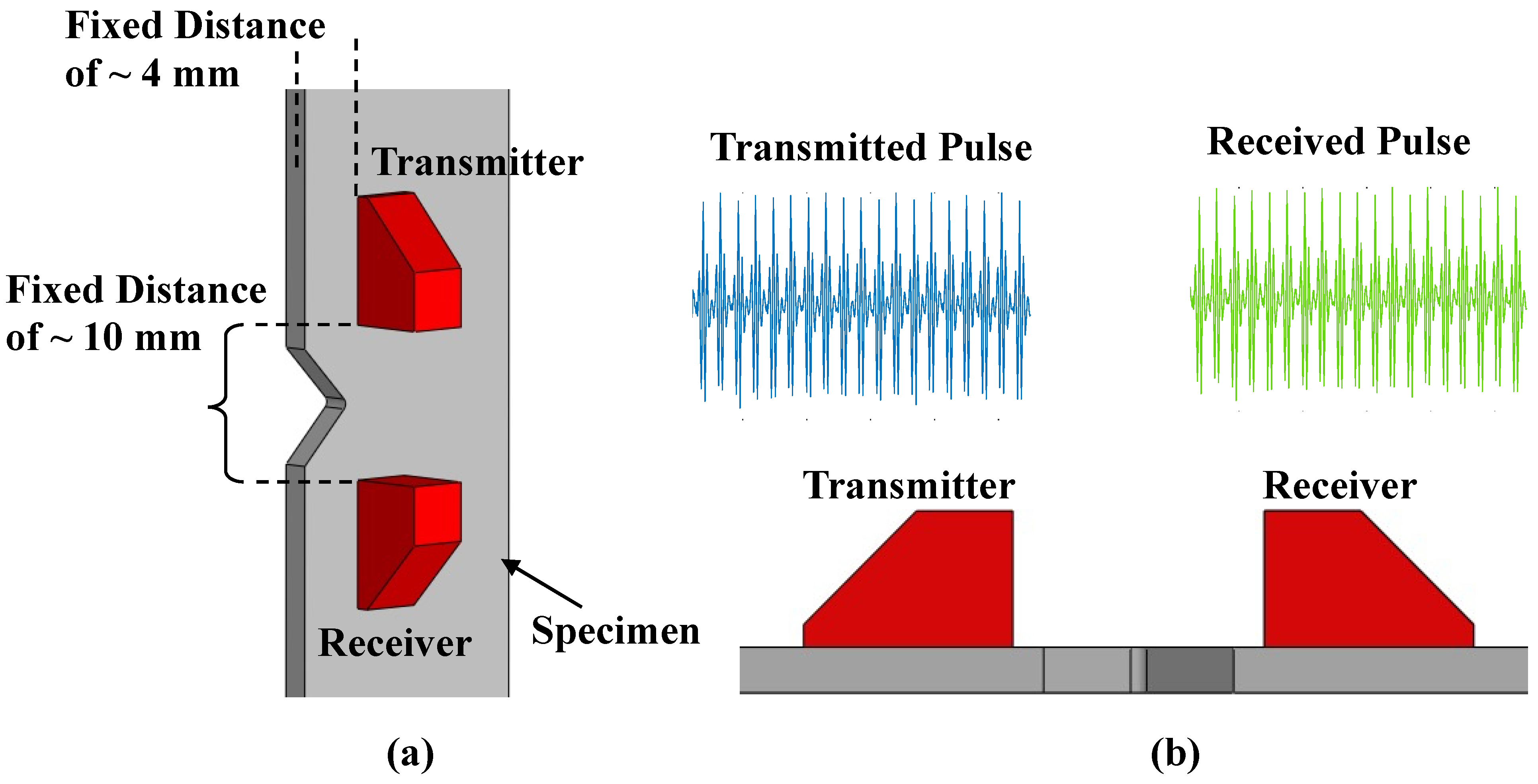
2.3.1. Ultrasonic Sensors

The capability of the ultrasonic sensors in detecting damage depends on the frequency at which the ultrasonic waves are emitted. From a length scale perspective, higher frequency leads to better capability in detecting small damage/defects. Past studies in the literature have used smaller frequencies (~350 kHz) and have, thus, focused on larger cracks, which are in the order of a few millimeters [14]. To move to a micron-scale detection for a large component as experimented in this paper, sensors having frequencies in the range of ~10 MHz would be theoretically conducive and, are commercially available.
A schematic showing the placement of the ultrasonic sensors on the specimens is shown in Figure 4a. The distance between the receiver and the transmitter is kept identical for all experiments. Similarly, the distance from the side edge of the specimens to the ultrasonic sensors is also identical for all experiments. The sensors are acquired from Olympus (Shinjuku, Tokyo, Japan) and are rated at a center frequency of 10 MHz. The angled wedges are rated at 45° and the sampling frequency for the data acquisition system is 100 MHz. Higher center frequency for the sensors is chosen for this study to enable finer crack detection. Figure 4b shows representative signals at the transmitter and the receiver ends.

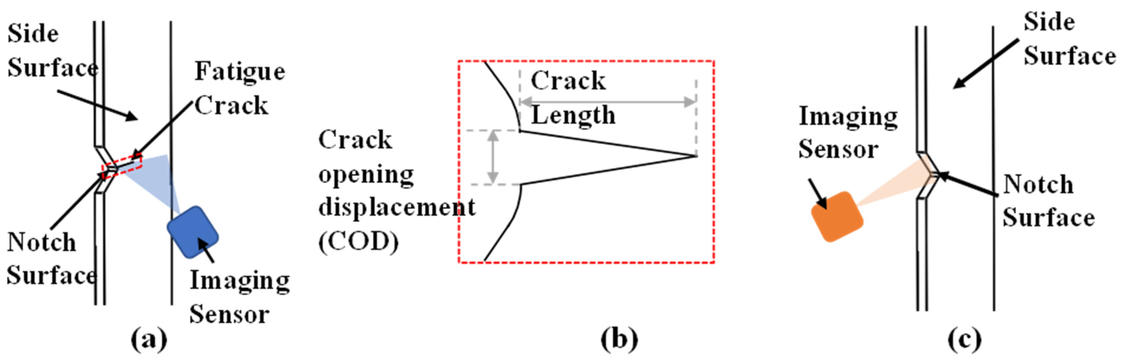
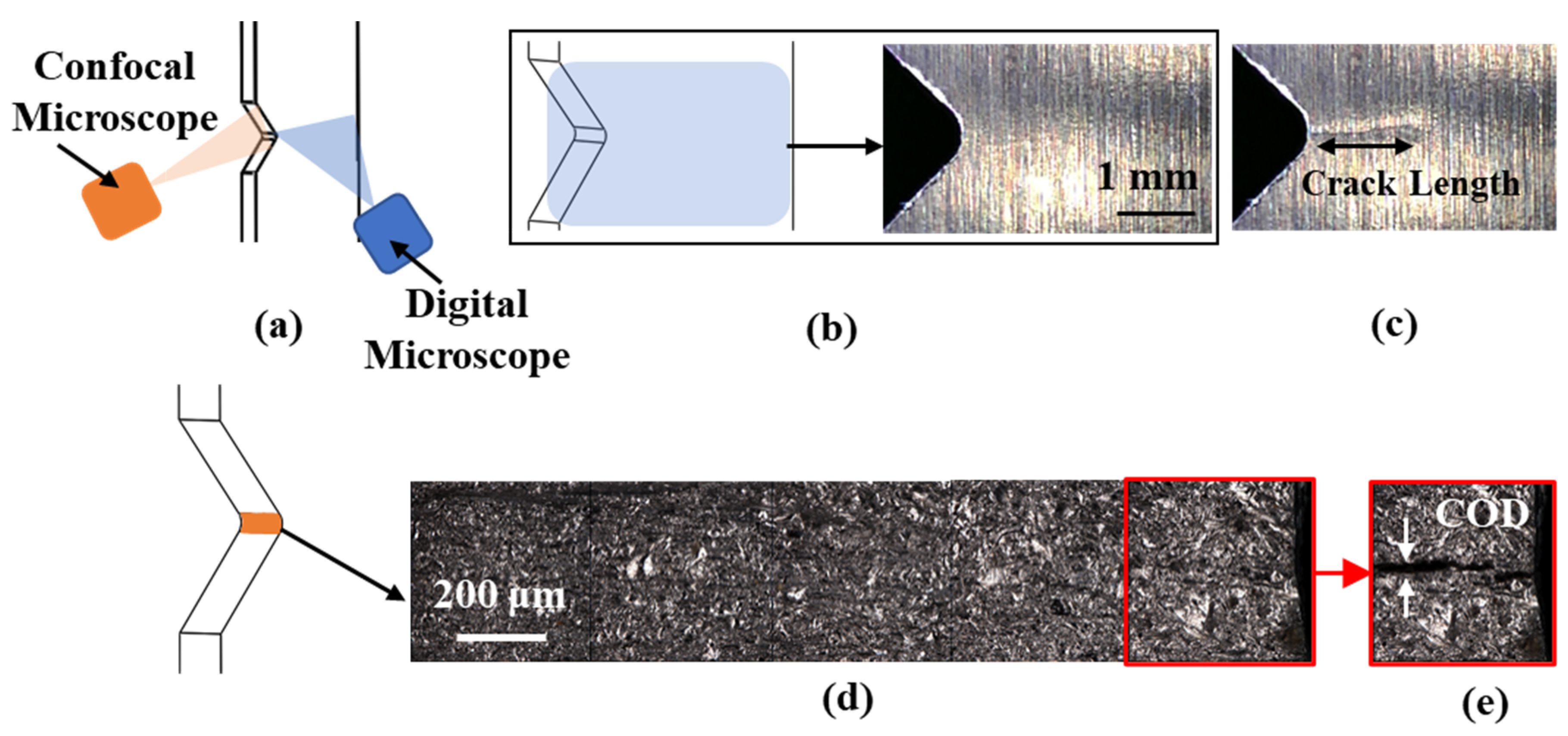
2.3.2. Confocal and Digital Microscope

To pinpoint the instant of fatigue damage initiation on ultrasonic receiver signals (or any time series signals), it is essential to have a visual insight to capture the cracks near the notch. To that end, the present study uses a dual-imaging setup to monitor the fatigue damage progression near the notch from two perpendicular orientations as shown in Figure 5a [26]. The model of the digital microscope used in the experiments is Dino-Lite Premier, which is a commonly used PC-based USB instrument [27]. It is capable of capturing features above a threshold of approximately 0.1 mm. The focus area of the microscope and a representative image is shown in Figure 5b. A corresponding image for a cracked specimen indicating the crack length is shown in Figure 5c. The imaging through the microscope is carried out at regular intervals during the scheduled stoppages from the MTS system. The crack length is measured using the DinoCapture 2.0: Microscope Imaging Software that is provided with the microscope.
The confocal microscope model, IF-SensorR25, belongs to the InfiniteFocus series manufactured by Bruker Alicona (Graz, Austria). The microscope uses a novel focus variation technology [28,29] enabling the procurement of high-resolution images across the depth of field. As compared to the digital microscope, this microscope is of a much higher resolution and is therefore suitable to observe COD, which is an order of magnitude smaller than the crack length. From an accuracy perspective, the microscope is capable to detect cracks with a COD of 3 μm. In the present study, the microscope is operated at a 50× resolution, having a field of view of 400 μm × 400 μm. The microscope is focused on the notch root. Since the thickness of the specimen is about six times larger than the maximum length captured by the microscope, the microscope is translated along the notch root to monitor the entire surface during each periodical stop in the fatigue test. Such a translation is achieved using a high-precision moving stage (Aerotech, Inc., Pittsburgh, PA, USA) on which the confocal microscope is mounted. The stage can handle movements up to a micrometer scale aiding in precise measurements during the fatigue test. A collage of all images capturing the entire notch root is also shown in Figure 5d. With subsequent damage progression, a representative cracked surface and COD corresponding to the 6th segment of the collage is highlighted in Figure 5e.

3. Integration of Symbolic Time-Series Analysis (STSA) with Machine Learning

The efficacy of the present research of developing a machine learning framework for damage detection depends on the capability of the time-series analysis algorithm. To fulfill all the objectives for damage detection, the algorithms need to be computationally efficient and savvy to deal with the ultrasonic signals that may be noisy. STSA has shown remarkable results [3] in dealing with such signals and, with minimal data. This section explains the basic algorithm for STSA and formulates the ensuing machine learning structure.

3.1. Symbolic Time-Series Analysis (STSA)

STSA is an amalgamation of the principles from symbolic dynamics, information theory, and pattern recognition. It is a statistical signal processing algorithm that works by filtering a signal to a symbolic domain [3]. The main objective for STSA is to convert the given signals into some measurable unique features that enable a comparison between multiple signals. This measurable feature with STSA is the state transition matrix (STM). The procedure to extract STM from a signal can be broadly divided into four steps that are depicted in Figure 6. A dummy signal comprising two periods of a cosine curve generated with 40 points is shown in Figure 6a. The first step towards generating an STM is the normalization and segmentation of the signal into discrete partitions. The four partitions, p, q, r, and s, are depicted in Figure 6a. The number of partitions depends on the practitioner with a higher number of partitions leading to a finer resolution for signal behavior but is often restricted by the total amount of training data volume. The normalization before partition serves two main objectives: (i) mitigation of the effect of noise and bias, and (ii) ensuring a fixed partition boundary across all signals. These partitions are assigned to separate symbols (for namesake) and the signal is then reduced to a symbolic chain corresponding to different partitions, as illustrated in Figure 6b. For creating partitions, there are several methods such as uniform, maximum entropy, and k-means [30] available in the open literature. Amongst these methods, the maximum entropy partitioning (MEP) scheme has been found to yield the best efficiency in predictions [3]. According to the set-theory formulation, A is the set of symbols, and its cardinality, | A | , is the number of partitions. For the cosine signal in Figure 6a, A = {p, q, r, s} and | A | = 4.
At the end of the symbolic transform step, the signal loses the time domain information and is solely existent in the discrete symbolic domain. To develop the analysis further, the symbol chain is treated as being analogous to a series of state transitions akin to the representations in the finite state automata (FSA) theory [31]. Such FSAs are commonly studied in the robotics community [32] and the present analysis merely draws an abstraction from this structure. For the symbol chain, the symbols (or a collection of symbols) can be treated as the states of the system. Correspondingly, the interactions can be shown through a state diagram (Figure 6c) by treating the symbols as states. Since the states and symbols can be distinct, the set of states is denoted by Q , and for the cosine series, Q is the same as A . With this ingenious abstraction of an FSA, several possibilities (such as the STM) for a unique feature can be exploited. Accordingly, the transitions in the state diagram are quantified using a probabilistic analysis. The ensuing probabilistic FSA (or PFSA) comprises a probability map (or morph function), π, which aids in computing the probability of transitioning between two states. Mathematically, the morph function is, therefore, a matrix. The morph function is equivalent to the state transition matrix (T) in the case where the number of symbols is equal to the number of states and is shown in Figure 6d for the cosine signal. It is to be noted that π and T can, in general, be different because the set of symbols and states can vary. The computation of the elements of π is done by counting the number of transitions from present states to the next symbols. If Nij is denoted as the number of transitions from ith state to jth symbol, then πij is computed as:
π i j = 1 + N i j | A | + k N i k
The subscript k varies through the number of symbols. With the presented case study for the signal, it is straightforward to verify the computation. For example, the readers can verify from the symbol chain in Figure 6b, that there are just two transitions from the state p to state q. Therefore, Npq = 2. Accordingly, k N pk = Npq + Npr + Nps + Npp = 2 + 0 + 0 + 9 = 11, and | A | = 4. Subsequently, πpq = (1 + 2)/(4 + 11) = 0.21. It should also be noted that the matrix is row-stochastic, meaning that the rows add up to 1. An important underlying assumption that makes the above formulation feasible is that of treating the entire concatenated signal as a Markov process. This assumption models the process such that the next state of the system is solely dependent on the present state. STSA builds on this definition and incorporates additional flexibility in allowing the dependence on the previous D steps. The parameter, D, is termed as the ‘depth’ of the analysis, and the resulting formulation is also called as the D-Markov machine to differentiate it from the conventional Markov process. This assumption holds for the analysis of the ultrasonic signals because the transition from a ‘healthy’ state to a ‘cracked’ state is gradual and corresponds to the cumulative buildup of damage. Due to this gradual change, an estimate on the state of the specimen can be made from a small change of the most recent information. This is yet another advantage of STSA with ultrasonics because it converts a cumulative process into an intermittently tractable process without the need for the entire history. More details on the mathematical foundation of PFSA can be found in several pieces of literature [33,34,35,36,37].

3.2. Machine Learning Framework

The STSA formulation decomposes the signal into the state transition matrix T, which acts as the primary feature of the signal. In addition to T, the standard deviation, σ, and the mean, μ can also be considered as features. Since their computation is inexpensive, they are included in the current formulation and computed using the mean and std functions in MATLAB®, respectively. Therefore, through STSA, any signal is decomposed into three features, viz. T, σ, and μ. To assess the state (i.e., ‘healthy’ or ‘cracked’) of a signal, these three feature definitions are required to be conditioned to some reference values that enable a comparison. Figure 7a schematically depicts the training process where the ‘healthy’ part of an ith training signal is decomposed into its corresponding three features: THi, σHi, and μHi. These features are averaged over the entire training data to generate TH, σH, and μH.
With the availability of these reference healthy features, i.e., TH, σH, and μH, the following composite metric ρi is defined for any ith test signal to assess its state (i.e., ‘healthy’ or ‘cracked’): ρ i = | | T i T H | e ,   σ i σ H ,   μ i μ H | e . Here, | | e denotes the Euclidean norm, and Ti, σi, and μi correspond to the individual features of the ith test signal. For a single signal window such as the cosine signal shown in Figure 6a, ρi is a scalar. During the experiment, with sequential computation of ρi for every incoming signal window, a time-series vector can be generated by stacking ρ i for every window as follows: ρ = [ ρ 1 ,   ρ 2 , ,   ρ i , , ρ n ] . This is the outcome of the STSA algorithm that is used to create a classifier between the ‘healthy’ and ‘cracked’ signals. Figure 7b shows the typical behavior of ρ plotted for a representative ultrasonic signal. To perform a classification between ‘healthy’ and ‘cracked’ signals, an appropriate optimal threshold (corresponding to the critical value of ρ), ρopt, needs to be established. An avenue to determine the optimal threshold is via computing the receiver operating characteristics curve (ROC) [38], such that the classification yields the lowest error in misclassifying the ‘healthy’ and ‘cracked’ signals. ROC curves plot the behavior of the true positive rate against the false-positive rate for a varying set of thresholds (e.g., ρ). In the current context, the true positive rate corresponds to the detection of a crack when the signal is actually ‘cracked’ and the false positive rate corresponds to an erroneous detection. The ROC curve for Figure 7b is shown in Figure 7c. On Figure 7b, the instance of damage detection is when ρ and ρopt intersect.
The value of ρopt estimated through ROC is expected to have some variability over all specimens. Therefore, to learn the best value of ρopt, a second round of training is performed using the training data. The schematic of this training procedure is shown in Figure 8a. The second set of training data is processed through STSA, and the extracted features are compared with the trained ‘healthy’ parameters using the metric defined in the preceding paragraphs. A vector of monotonically increasing ρi is then calculated for the training data. Using ROC curves, ρopt for the training data is calculated. The final trained value of ρopt is then computed as an arithmetic mean of all the individual thresholds and is indicated by ρfinal. With the computation of ρfinal, the training phase of the procedure is concluded. To summarize, the training phase computes four parameters viz. ρfinal, TH, σH, and μH. The calculation of ρfinal and its effectiveness in predicting a failure is accompanied by a decision-making process, as shown in Figure 8b. A test signal is processed with STSA and then compared with the trained parameters, leading to the composite metric ρi. ρi is then compared with ρopt, and depending on its magnitude, the new signal is labeled as ‘healthy’ or ‘cracked’.

4. Results and Discussion

15 U-notched and 15 V-notched specimens are tested, and the corresponding ultrasonic time-series signal data, confocal images, and digital images are collected. The following sections explain the results and the subsequent crack detection capabilities of the proposed algorithm.

4.1. Fatigue Failure Progression

Using the dual-imaging setup, the experiments capture COD at the notch root with the confocal microscope. The crack length is characterized on the side of the notch with the digital microscope. During the fatigue failure, independent data from the microscopes reveal three distinct regimes of failure chronology as illustrated in Figure 9. The ‘healthy’ regime corresponds to the duration where no instance of a crack is observed in either of the microscopes, as depicted in Figure 9a,b. After persistent loading, multiple fine cracks are observed at the notch root through the confocal microscope (Figure 9c,d). This initial crack corresponds to a COD of ~3 μm and the identification of these cracks becomes possible due to the high resolution of the confocal microscope. This emergence of cracks is termed as the start of the crack coalescence (CC) regime. It is important to note that the digital microscope has no apparent indication of damage. Going further with the loading, the crack coalescence regime culminates with a dominant crack that is ubiquitously observed on both the microscopes (Figure 9e,f). This instance of a dominant crack emergence is termed as the start of the crack propagation (CP) regime. Owing to the resolution of the digital microscope, the crack length at the instant of detection corresponds to ~0.2 mm. In the later stages of the test, both the features show significant growth, as depicted in Figure 9g,h.
To illustrate the combined behavior, Figure 10 numerically plots both features against the normalized fatigue life of a representative V-notched specimen. Using this distinct observation, the plot highlights three main regimes which are henceforth defined as ‘healthy’, ‘crack coalescence’, and ‘crack propagation’. Based on the short- and long-crack bifurcation that has been used in many of the past pieces of literature [39], a crack length of the order of 1 mm can be considered as the initiation to a long-crack regime. In the subsequent sections, the capability of crack detection is therefore quantified for crack lengths of 1 mm as well. With respect to the fatigue life, the V-notched specimens sustain up to 65,000 cycles before fracture as opposed to 40,000 cycles for the U-notched specimens. The variability in the fatigue life across both sets of specimens is shown in Figure 11. Broadly, the larger fatigue life of the V-notch specimens can be attributed to the lower stress concentration near the notch root. The variability in the CC and CP regimes is also shown against the fatigue life in Figure 11. On average, it is observed that the CC regime sets in at around 30% and 45% of the fatigue life in U-notch and V-notch specimens, respectively. Similarly, the CP region initiates at 51% and 58% of the fatigue life in U-notch and V-notch specimens, respectively. An ability to detect cracks in the CC regime thus enables an additional ~13–21% fatigue life (i.e., number of load cycles) buffer for maintenance purposes for the V- and U-notched specimens, respectively. This analysis, therefore, sets up the basis for the benefits of an early-stage crack detection. The next sections evaluate the combined capability of the ultrasonic sensors and STSA to detect the emergence of cracks for CC, CP, and CP > 1 mm regimes.

4.2. Ultrasonic Time-Series Signal

During the entirety of the fatigue life of the specimens, the ultrasonic receiver continuously accrues the time-series signal carrying the signature of the fatigue damage. Figure 12a shows the behavior of the time-series data obtained from the receiver and segregated into the four predefined regimes (i.e., healthy, CC, CP, and CP > 1 mm). The signal is plotted against the timesteps which correspond to the number of data points that constitute the signal. Since the signal is regularly sampled at a very high rate (100 MHz), the number of points through a complete fatigue experiment of one specimen amounts to a time-series consisting of ~105 data points. Therefore, by experimenting with 15 specimens, a total of ~15 × 105 points are accrued for each notch type, proving a rich resource to execute the machine learning algorithm described in the upcoming sections. As opposed to the microscopes which can directly show the fatigue cracks, the ultrasonic signals are implicitly dependent on the in-sync imaging capabilities for accurate calibration. The points of transition between the healthy, CC, CP, and CP > 1 mm phases are obtained from the transitions observed in Figure 10. Zoomed-in versions of the signals in these three regimes are shown in Figure 12b–d. The ultrasonic signal attenuates significantly as the crack size increases.
A training–testing split of 60%–40% is used for both types of specimens (i.e., ‘U’ and ‘V’ notches). Owing to this ratio, the training of STSA is accomplished using the signal data obtained from 9 (out of 15) specimens and the testing is performed on the signal data obtained from the remaining 6 specimens. A comparatively higher (6) number of testing specimens ensures an unbiased estimate of the accuracy of the algorithm and is beneficial due to the larger variability exhibited during a fatigue test. The hyperparameters (# of partitions (N), depth (D), and partitioning scheme) are optimized and the STSA metrics (TH, σH, and μH) are then obtained to create a ‘healthy’ reference. Based on an in-depth understanding of STSA [19], the hyperparameters used in this work are N = 10 and D = 1, with MEP partitioning. It is often possible to bias the results of such machine learning framework by a biased train-test split. To avoid such biases, a hold-out validation using 20 iterations of random train-test splits is performed and the average accuracy across all the iterations is presented.

4.3. Regime-Specific Fatigue Crack Detection

Using the STSA-based machine learning framework established in Section 3, the crack detection capability using the ultrasonic response is now evaluated for each of the specific regimes (CC, CP, and CP > 1 mm). In general, the application of STSA begins with the generation of labeled training and testing datasets from the pool of 15 specimens for each type of notch. The datasets are created by using a moving window of fixed width, each encompassing a predefined number of ultrasonic signals. Figure 12b–d demonstrates the example datasets for the healthy and the cracked regime, each consisting of 20 signals. Due to the nature of defining the labeled datasets, for each regime, the bifurcation between a ‘healthy’ signal and a ‘cracked’ one is defined individually, as shown in Figure 13. The original signal with three regimes (Figure 13a) is converted to a labeled signal, e.g., ‘healthy’ and ‘cracked’, with varying transition points as illustrated in Figure 13b–d. Accordingly, detecting a cracked specimen in the CC regime would correspond to the most challenging goals among the alternatives. In the CP regime, the detection goal becomes simpler. As the crack length increases, a significant amount of signal attenuation is observed, which is much easier to detect.

4.3.1. Fatigue Crack Detection in the CC Regime

For analysis in the CC regime, the transition point corresponding to Figure 13b is used. Figure 14a,b shows the variation of ρ superimposed on an ultrasonic signal for a representative U- and V-notched specimen, respectively. As indicated earlier, the location where the curve for ρ intersects the ρopt line corresponds to the instance of crack detection by the algorithm. The performances exhibited by the ROC for 9 test specimens for each notch type are plotted in Figure 14c,d. Intuitively, ρopt is chosen as the one which maximizes the accuracy of classification.
The distribution of all ρopt values derived from all the training data is shown in Figure 15a. The final ρopt (i.e., ρfinal) used further in the analysis is calculated as the statistical mean of all ρopt values. For the U-notched specimens, ρfinal is 2.36, and for the V-notched specimens, it is 2.93. The testing performance for representative U- and V-notched specimens is shown in Figure 15b,c using ρfinal. It is important to note that while classifying the data from the test specimens, the training parameters are the only information that is used. In this manner, through the training paradigm, any new ultrasonic signal can be tested for its health using just four parameters, viz. TH, σH, μH, and ρfinal. The ensuing accuracies, through a hold-out validation, are shown through boxplots in Figure 16 for both sets of notches. The U-notch specimens demonstrate an average training and testing accuracy of 79.82% and 68.18%, respectively, whereas the V-notch specimens exhibit a training and testing accuracy of 81.94% and 74.12%, respectively in detecting cracks in the CC regime. The variation in testing accuracy is larger as compared to training because the testing specimens use the optimal thresholds based on the training specimens.

4.3.2. Fatigue Crack Detection in the CP and CP > 1 Regimes

Following a chronology identical to the CC section, the efficacy of the proposed algorithm is now evaluated for the CP regime. The generation of the datasets and the training methodology follow the same steps as used in the preceding section. The only difference with the CP regime is that all the data appearing after the CP detection are classified as cracked, as shown in Figure 13c. The threshold distributions for both sets of specimens are shown in Figure 17a. The newly trained thresholds for the CP regime are 3.82 and 3.07 for the U- and V-notched specimens, respectively. Like the CC regime, a hold-out validation analysis is performed over 20 random 60%–40% splits of train-test datasets for the CP regime as well. The variation in accuracy of the training and testing datasets is shown in Figure 17b,c. The U-notched specimens demonstrate an average training and testing accuracy of 88.3% and 81.94%, respectively, whereas the V-notched specimens exhibit a training and testing accuracy of 91.85% and 85.62%, respectively in detecting cracks in the CP regime. The distributions also depict the outliers in the prediction accuracy across different iterations with the testing accuracy of the V-notched specimens ranging from 54% to 87%, which is compensated by using such a hold-out validation.
From the preceding analysis of crack detection in the CC and CP regime, it is evident that the ultrasonic sensors are more accurate in detecting the larger of the two cracks (CP regime). From the behavior of the ultrasonic attenuation, it is also clear that beyond the CP regime, the signal attenuation is much more significant, and crack detection can be achieved with higher accuracy. To quantify this observation, an analysis of the accuracy of detection at a crack length of 1 mm in the CP regime is performed. Figure 18 shows the variation of average accuracy across 20 iterations for both the specimens using the same hold-out validation scheme as used before. Using this variation, the average training accuracy of detecting a crack of length 1 mm is calculated to be 95.48% and 97.76% for the U- and V-notched specimens, respectively. The testing accuracies are 90.07% and 91.38% for the U- and V-notched specimens, respectively. Although, this clearly demonstrates the excellent capability of ultrasonic sensors in detecting larger cracks, the caveat, from a maintenance perspective, is the smaller reaction time for taking preventive measures. In this problem, with 1 mm crack, the specimens have already completed ~80% of their fatigue lives which is fairly high as compared to ~ 30%–50% fatigue life accrued before the CC regime.

5. Summary, Conclusions, and Future Work

The article primarily presents the efficacy of a time-series algorithm using STSA integrated with a machine learning-based architecture for fatigue crack detection in a popular aluminum alloy, Al7075. Two sets of Al7075 specimens (15 each) are studied. The fatigue propagation, based on a dual-imaging setup, is divided into three main regimes, (i) healthy, (ii) crack coalescence (CC), and (iii) crack propagation (CP). The CC regime is characterized by the detection of a crack with COD of ~3 μm. The CP regime is characterized by the detection of a crack with a length of ~0.2 mm. The performance of the STSA algorithm for crack detection is studied for CC and CP regimes. In the CP regime, the performance is also analyzed for a longer crack corresponding to CP > 1 mm. The training and testing accuracies observed for all the regimes and specimens are summarized in Figure 19. Overall, the performance of STSA for the CC regime is observed to be lower than the CP regime, indicating the difficulty in detecting finer cracks with COD ~3 μm. In the CP regime for larger crack lengths (>1 mm), the performance of STSA is beyond 90%. The contributions of the current paper are succinctly documented in Table 2.
The presented method is particularly useful due to the low amounts of data (based on 15 specimens) needed for the trained model as compared to neural network-based analysis. The computation time observed during the training is negligible (~1 min on an Intel® Core™ i7-4790 CPU@ 3.60 GHz with 16 GB RAM). The computation also does not require a GPU, which is almost essential for all neural network-based models. An important outcome of the research that needs to be addressed in the future is the low accuracy of detection in the CC regime. From the progression of the data, it is evident that ultrasonic signals show minimal changes while transitioning to the CC regime. Therefore, to address this issue, the research can either be directed toward superior data analysis algorithms or improved sensing techniques. From a data analysis perspective, several complex algorithms such as auto-encoders, long short-term memory, and recurrent neural networks will be investigated in the future to assess the improvement in accuracy. It is plausible that these techniques may not achieve the required accuracy if the sensors are unaffected by the minuscule damages observed through the confocal microscope. Therefore, a logical approach to improve the accuracy is to use advanced ultrasonic sensors that detect the nonlinear effects during the fatigue failure evolution [15]. In the future, non-linear ultrasonics will be explored to investigate their efficacy in detecting finer cracks. The investigation in the current research is focused on Al7075. In the future, other critical structural materials such as steels will also be investigated.

Author Contributions

Conceptualization, A.B. and S.D.; methodology, S.D., C.B., A.B. and A.R.; software, S.D. and C.B.; validation, S.D. and C.B.; formal analysis, S.D.; investigation, S.D.; resources, A.B. and A.R.; data curation, S.D.; writing—original draft preparation, S.D. and A.B.; writing—review and editing, A.B. and A.R.; visualization, S.D. and C.B.; supervision, A.B.; project administration, A.B.; funding acquisition, A.B. and A.R. All authors have read and agreed to the published version of the manuscript.

Funding

The work reported in this paper was supported in part by the Department of Mechanical Engineering at the Pennsylvania State University, University Park, PA 16802 and in part by the U.S. Air Force Office of Scientific Research (AFOSR) under Grant No. FA9550-15-1-0400. The APC was funded by the Machines Editorial Office.

Institutional Review Board Statement

Not applicable.

Informed Consent Statement

Not applicable.

Data Availability Statement

The datasets generated during and/or analyzed during the current study are available from the corresponding author on reasonable request.

Acknowledgments

The authors would like to thank Eric Keller and Kevin Fisher for their help with the ultrasonic testing, MTS fatigue testing apparatus, and the confocal microscope. The authors are indebted to Christopher Hirsh and Nicholas Moore for their help in resolving IT related issues.

Conflicts of Interest

The authors declare that they have no known competing financial interests or personal relationships that could have appeared to influence the work reported in this paper.

References

  1. Suresh, S. Fatigue of Materials; Cambridge University Press: Cambridge, UK, 1998. [Google Scholar]
  2. Inman, D.J.; Farrar, C.R.; Junior, V.L.; Junior, V.S. Damage Prognosis: For Aerospace, Civil. and Mechanical Systems; John Wiley & Sons: New York, NY, USA, 2005. [Google Scholar]
  3. Gupta, S.; Ray, A.; Keller, E. Online fatigue damage monitoring by ultrasonic measurements: A symbolic dynamics approach. Int. J. Fatigue 2007, 29, 1100–1114. [Google Scholar] [CrossRef]
  4. Karimian, S.F.; Modarres, M.; Bruck, H.A. A new method for detecting fatigue crack initiation in aluminum alloy using acoustic emission waveform information entropy. Eng. Fract. Mech. 2020, 223, 106771. [Google Scholar] [CrossRef]
  5. Papazian, J.M.; Nardiello, J.; Silberstein, R.P.; Welsh, G.; Grundy, D.; Craven, C.; Evans, L.; Goldfine, N.; Michaels, J.E.; Michaels, T.E.; et al. Sensors for monitoring early stage fatigue cracking. Int. J. Fatigue 2007, 29, 1668–1680. [Google Scholar] [CrossRef]
  6. Leong, W.H.; Staszewski, W.J.; Lee, B.C.; Scarpa, F. Structural health monitoring using scanning laser vibrometry: III. Lamb waves for fatigue crack detection. Smart Mater. Struct. 2005, 14, 1387. [Google Scholar] [CrossRef]
  7. Kong, X.; Li, J.; Collins, W.; Bennett, C.; Laflamme, S.; Jo, H. A robust signal processing method for quantitative high-cycle fatigue crack monitoring using soft elastomeric capacitor sensors. In Proceedings of the Sensors and Smart Structures Technologies for Civil, Mechanical, and Aerospace Systems, Portland, OR, USA, 26–29 March 2017; Volume 10168, p. 101680B. [Google Scholar]
  8. Dharmadhikari, S.; Basak, A. Energy dissipation metrics for data-driven fatigue damage detection in the short crack regime for aluminum alloys. In Turbo Expo: Power, Land, Sea, and Air; American Society of Mechanical Engineers; 7 June 2021; Volume 85031, p. V09BT26A004.
  9. Anderson, T.L. Fracture Mechanics: Fundamentals and Applications; CRC Press: Boca Raton, FL, USA, 2017. [Google Scholar]
  10. Danzl, R.; Helmli, F.; Scherer, S. Focus variation—A new technology for high resolution optical 3D surface metrology. In Proceedings of the 10th International Coneference of the Slovenian Society for Non-Destructive Testing, Ljubljana, Slovenia, 1–3 September 2009; pp. 481–491. [Google Scholar]
  11. Dharmadhikari, S.; Basak, A. Evaluation of Early Fatigue Damage Detection in Additively Manufactured AlSi10Mg. In Proceedings of the Annual International Solid Freeform Fabrication Symposium, Virtual, 2–4 August 2021. [Google Scholar]
  12. Mitra, M.; Gopalakrishnan, S. Guided wave based structural health monitoring: A review. Smart Mater. Struct. 2016, 25, 53001. [Google Scholar] [CrossRef]
  13. Rose, J.L. Ultrasonic Guided Waves in Solid Media; Cambridge University Press: Cambridge, UK, 2014. [Google Scholar]
  14. Cho, H.; Lissenden, C.J. Structural health monitoring of fatigue crack growth in plate structures with ultrasonic guided waves. Struct. Heal. Monit. 2012, 11, 393–404. [Google Scholar] [CrossRef]
  15. Matlack, K.H.; Kim, J.Y.; Jacobs, L.J.; Qu, J. Review of Second Harmonic Generation Measurement Techniques for Material State Determination in Metals. J. Nondestruct. Eval. 2015, 34, 273. [Google Scholar] [CrossRef]
  16. Herrera, R.H.; Orozco, R.; Rodriguez, M. Wavelet-based deconvolution of ultrasonic signals in nondestructive evaluation. J. Zhejiang Univ. A 2006, 7, 1748–1756. [Google Scholar] [CrossRef] [Green Version]
  17. Bagnall, A.; Lines, J.; Bostrom, A.; Large, J.; Keogh, E. The great time series classification bake off: A review and experimental evaluation of recent algorithmic advances. Data Min. Knowl. Discov. 2017, 31, 606–660. [Google Scholar] [CrossRef] [Green Version]
  18. Bhattacharya, C.; Dharmadhikari, S.; Basak, A.; Ray, A. Early detection of fatigue crack damage in ductile materials: A projection-based probabilistic finite state automata approach. ASME Lett. Dyn. Syst. Control. 2021, 1, 41003. [Google Scholar] [CrossRef]
  19. Mukherjee, K.; Ray, A. State splitting and merging in probabilistic finite state automata for signal representation and analysis. Signal. Process. 2014, 104, 105–119. [Google Scholar] [CrossRef]
  20. Available online: http://asm.matweb.com/search/SpecificMaterial.asp?bassnum=MA7075T6 (accessed on 5 May 2019).
  21. E466-07, Standard Practice for Conducting Force Controlled Constant Amplitude Axial Fatigue Tests of Metallic Materials; ASTM International: West Conshohocken, PA, USA, 2007.
  22. N’Diaye, A.; Hariri, S.; Pluvinage, G.; Azari, Z. Stress concentration factor analysis for notched welded tubular T-joints. Int. J. Fatigue 2007, 29, 1554–1570. [Google Scholar] [CrossRef]
  23. Kurowski, P. Engineering Analysis with SolidWorks Simulation 2013; SDC publications: Mission, KS, USA, 2013. [Google Scholar]
  24. Boud, F.; Loo, L.F.; Kinnell, P.K. The Impact of Plain Waterjet Machining on the Surface Integrity of Aluminium 7475. Procedia CIRP 2014, 13, 382–386. [Google Scholar] [CrossRef] [Green Version]
  25. Albedah, A.; Bouiadjra, B.B.; Mohammed, S.; Benyahia, F. Fractographic analysis of the overload effect on fatigue crack growth in 2024-T3 and 7075-T6 Al alloys. Int. J. Miner. Metall. Mater. 2020, 27, 83–90. [Google Scholar] [CrossRef]
  26. Dharmadhikari, S.; Keller, E.; Ray, A.; Basak, A. A dual-imaging framework for multi-scale measurements of fatigue crack evolution in metallic materials. Int. J. Fatigue 2021, 142, 105922. [Google Scholar] [CrossRef]
  27. Siddiqui, S.F.; Fasoro, A.A.; Cole, C.; Gordon, A.P. Mechanical Characterization and Modeling of Direct Metal Laser Sintered Stainless Steel GP1. J. Eng. Mater. Technol. 2019, 141, 031009. [Google Scholar] [CrossRef]
  28. Jiang, X.; Tong, Z.; Li, D. On-Machine Measurement System and Its Application in Ultra-Precision Manufacturing. Precis. Mach. 2020, 563–599. [Google Scholar] [CrossRef]
  29. Danzl, R.; Helmli, F.; Scherer, S. Focus Variation--a Robust Technology for High Resolution Optical 3D Surface Metrology. Stroj. Vestn. J. Mech. Eng. 2011, 57, 245–256. [Google Scholar] [CrossRef] [Green Version]
  30. Bishop, C.M. Pattern Recognition and Machine Learning; Springer: Berlin/Heidelberg, Germany, 2006. [Google Scholar]
  31. Veanes, M. Applications of symbolic finite automata. In Proceedings of the International Conference on Implementation and Application of Automata, Halifax, NS, Canada, 16–19 July 2013; pp. 16–23. [Google Scholar]
  32. Hettiarachchi, S.; Spears, W.M.; König, L.; Mostaghim, S.; Schmeck, H. Decentralized evolution of robotic behavior using finite state machines. Int. J. Intell. Comput. Cybern. 2009, 2, 695–723. [Google Scholar]
  33. Piccardi, C. On parameter estimation of chaotic systems via symbolic time-series analysis. Chaos An. Interdiscip. J. Nonlinear Sci. 2006, 16, 43115. [Google Scholar] [CrossRef]
  34. Makki Alamdari, M.; Samali, B.; Li, J.; Lu, Y.; Mustapha, S. Structural condition assessment using entropy-based time series analysis. J. Intell. Mater. Syst. Struct. 2017, 28, 1941–1956. [Google Scholar] [CrossRef]
  35. Makki Alamdari, M.; Samali, B.; Li, J. Damage localization based on symbolic time series analysis. Struct. Control. Heal. Monit. 2015, 22, 374–393. [Google Scholar] [CrossRef] [Green Version]
  36. Kumar, S.; Pecht, M.G. Health Monitoring of Electronic Products Using Symbolic Time Series Analysis. In Proceedings of the AAAI Fall Symposium: Artificial Intelligence for Prognostics, Arlington, VA, USA, 9–11 November 2007; pp. 73–80. [Google Scholar]
  37. Brida, J.G. Multiple Regimes Model Reconstruction Using Symbolic Time Series Methods. Int. J. Appl. Math. Stat. 2006, 5, 19–40. [Google Scholar]
  38. Poor, H.V. An Introduction to Signal Detection and Estimation; Springer Science & Business Media: New York, NY, USA, 2013. [Google Scholar]
  39. Schijve, J. Fatigue of Structures and Materials; Springer Science & Business Media: New York, NY, USA, 2001. [Google Scholar]
Figure 1. (a) Schematic of a representative fatigue specimen with a one-sided V-notch illustrating the view area of the imaging sensors for fatigue crack detection; (b) Characterization of the crack length and the crack opening displacement (COD) used in the current work; (c) A potential alternative orientation of an imaging sensor to observe COD.
Machines 09 00211 g001
Figure 2. Geometry of the one-sided (a) V-notched; (b) U-notched specimens (all dimensions are in mm).
Machines 09 00211 g002
Figure 3. (a) Custom-built fatigue testing apparatus consisting of an MTS 831.10 servo-hydraulic frame, a confocal microscope mounted on a moving stage, and a digital microscope; (b) A zoomed-in view of the apparatus showing the orientation of the microscopes, the specimen, and the mounted ultrasonic transducers.
Machines 09 00211 g003
Figure 4. (a) A schematic (not to scale) showing the placement of the ultrasonic sensors on the specimens; (b) An alternate view of the specimens and the sensors. Representative transmitted and received signals are also illustrated.
Machines 09 00211 g004
Figure 5. (a) A schematic of the specimen illustrating the viewing areas of the digital and confocal microscopes; (b) A typical image area captured by the digital microscope and the corresponding image of a representative specimen; (c) A cracked version of the specimen as captured by the digital microscope indicating the crack length; (d) The region of interest of the confocal microscope with a collage of six individual images covering the entire notch root of a representative specimen; (e) An image of the 6th segment (extreme right of (d)) of the collage showing the formation of a fatigue crack depicting the COD.
Machines 09 00211 g005
Figure 6. Steps in symbolic time-series analysis. (a) a dummy signal (cosine) with 40 points and four partitions; (b) the symbolic chain filtered from the signal; (c) a state diagram between four states from the partitions; (d) the state transition matrix showing the probability of transition between the current state and next state in the signal; (e) The state transition matrix in (d) is depicted as a 3D plot.
Machines 09 00211 g006
Figure 7. (a) Framework for training the healthy features (TH, σH, and μH) using STSA; (b) A typical nature of ρ as observed through the analysis (for representative purposes) indicating the optimal threshold (ρopt); (c) The corresponding ROC curve.
Machines 09 00211 g007
Figure 8. (a) Training algorithm for obtaining the optimal threshold; (b) Decision-making process for a test signal using the trained STSA model.
Machines 09 00211 g008
Figure 9. The chronology of failure as observed by the microscopes for a representative V-notched specimen—(a,b) a healthy specimen, (c,d) crack coalescence regime where fine cracks (~3 μm) appear at the notch root, (e,f) the cracks coalesce, and a single crack is observed at the notch root and on the side of the specimen, and (g,h) crack growth continues. The arrows indicate the emergence of a crack on the images. In (b,d,h), images on the top row are obtained from the digital microscope, and on the bottom row, they are obtained from the confocal microscope. The images obtained from the U-notched specimens are similar and are excluded for brevity.
Machines 09 00211 g009
Figure 10. The variation of crack length and COD against the normalized fatigue life divided into three regimes, viz. healthy, crack coalescence (CC), and crack propagation (CP). The bifurcation of the CP regime beyond the crack length of 1 mm indicated by CP > 1 mm is also highlighted. The data obtained from the U-notched specimens is similar and is excluded for brevity.
Machines 09 00211 g010
Figure 11. Distribution of the total fatigue life (or load cycles) in the CC, CP, and fracture regimes with respect to the total number of load cycles for the (a) U-notched; (b) V-notched specimens. The red lines denote the medians of the distribution.
Machines 09 00211 g011
Figure 12. (a) Ultrasonic receiver data for a representative U-notched specimen depicting the four regimes, viz. healthy, crack coalescence (CC), crack propagation (CP), and crack length exceeding 1 mm (CP > 1 mm). Zoomed-in views showing the ultrasonic signal in (b) healthy, (c) CC, and (d) CP regimes. The CP > 1 mm regime is marked on (a). The V-notched data are similar and are excluded for brevity.
Machines 09 00211 g012
Figure 13. (a) The original ultrasonic signal depicting four different regimes. The labeled data for the (b) CC, (c) CP, and (d) CP > 1 mm regimes, illustrating the transition point between a healthy and cracked regime.
Machines 09 00211 g013
Figure 14. Performance of the training algorithm superimposed on a representative (a) U-notched and (b) V-notched ultrasonic time-series signal in the CC regime. The values of ρ and ρopt are plotted on the right axis. ROC curves for 9 individual (c) U-notched and (d) V-notched training specimens in the CC regime.
Machines 09 00211 g014
Figure 15. (a) Distribution ρopt for both sets of specimens in the CC regime. Performance of the testing algorithm on a representative (b) U-notched and (c) V-notched specimen in the CC regime. The red line in (a) denotes the medians of the distributions.
Machines 09 00211 g015
Figure 16. Average training and testing accuracy across all hold-out-based validation iterations for (a) U-notched and (b) V-notched specimens in the CC regime. The red lines denote the medians of the distributions.
Machines 09 00211 g016
Figure 17. (a) Optimal threshold distribution for both sets of specimens for the CP regime. Average training and testing accuracy across all hold-out-based validation iterations for (b) U-notched and (c) V-notched specimens in the CP regime. The red lines denote the medians of the distributions.
Machines 09 00211 g017
Figure 18. Average training and testing accuracy across all hold-out-based validation iterations for (a) U-notched and (b) V-notched specimens in the CP > 1 mm regime. The red lines denote the medians of the distributions.
Machines 09 00211 g018
Figure 19. Summary of the training and testing accuracies in the CC and CP regimes for the U- and V-notched specimens.
Machines 09 00211 g019
Table 1. A comparison of the crack detection capabilities for various imaging and sensing techniques.
Fatigue Crack Detection Paradigm
Sensor Type (Detection Sensor + Imaging Sensor)Operational Principle of the Detection SensorData Analysis AlgorithmCapability of Detection Using Image CalibrationReference
Ultrasonic + Digital/OpticalChange in material impedance or attenuation due to crack growthSTSA~0.2 mm
(crack length)
[3]
Acoustic Emission + OpticalChange in ultrasonic stress waves released during loadingInformation entropy~0.25 mm
(crack length)
[4]
LDV + DigitalChange in characteristic frequency and mode-shapes during operationPeak-to-peak amplitude~0.3 mm
(crack length)
[6]
Strain Gauge + DigitalLocal plastic deformationPeak-to-peak Amplitude~0.9 mm
(crack length)
[7]
Eddy Current + DigitalChange in conductivityChange in conductivity~0.5 mm
(crack length)
[5]
Table 2. The contributions of the current article with the methods described in Table 1.
Contribution of the Article
Sensor Type (Detection Sensor + Imaging Sensor)Sensor Operational PrincipleData Analysis TechniqueCapability of Detection Using Image CalibrationReference
Ultrasonic + Confocal + DigitalChange in material impedance or attenuation due to crack growthSTSA + Machine Learning~0.2 mm (crack length) with ~82% testing accuracy
~3 μm (COD) with ~ testing 71% accuracy
Current
Publisher’s Note: MDPI stays neutral with regard to jurisdictional claims in published maps and institutional affiliations.

