Article

Gear Teeth Deflection Model for Spur Gears: Proposal of a 3D Nonlinear and Non-Hertzian Approach

1
Politecnico di Torino, Corso Duca degli Abruzzi 24, 10129 Torino, Italy
2
GeDy TrAss s.r.l., Via Vincenzo Vela 42, 10128 Torino, Italy
*
Author to whom correspondence should be addressed.
These authors contributed equally to this work.
Machines 2021, 9(10), 223; https://doi.org/10.3390/machines9100223
Submission received: 26 August 2021 / Revised: 23 September 2021 / Accepted: 25 September 2021 / Published: 30 September 2021
(This article belongs to the Section Machine Design and Theory)

Abstract

:
In this paper, a three-dimensional model for the estimation of the deflections, load sharing attributes, and contact conditions will be presented for pairs of meshing teeth in a spur gear transmission. A nonlinear iterative approach based on a semi-analytical formulation for the deformation of the teeth under load will be employed to accurately determine the point of application of the load, its intensity, and the number of contacting pairs without a priori assumptions. At the end of this iterative cycle the obtained deflected shapes are then employed to compute the pressure distributions through a contact mechanics model with non-Hertzian features and a technique capable of obtaining correct results even at the free edges of the finite length contacting bodies. This approach is then applied to a test case with excellent agreement with its finite element counterpart. Finally, several results are shown to highlight the influence on the quasi-static behavior of spur gears of different kinds and amounts of flank and face-width profile modifications.

1. Introduction

Due to their inherent nature, load and stiffness fluctuations are the main source of excitation and cause of failure in geared transmissions [1,2,3]. Early experimental works from the Japanese school highlighted the interesting dynamic features of those systems, analyzing their torsional behavior including other sources such as profile errors or modifications [4,5,6,7,8]. At first, the dynamic factor (DF) was used to characterize and explain certain types of failures [9] by comparing the dynamic loads in operation with those under static conditions. Vibrations and impacts can certainly be traced back to variations in the input torque depending on the machine characteristics [10,11,12], but the time-varying mesh stiffness (TVMS) was quickly found to be a key player [13]. Indeed, the stiffness of an engaging gear pair changes continuously due its nature and can generate self-excited vibrations which led many researches in the study of the transmission error (TE). Over the years several methods have been proposed, starting from integral approaches [14,15] or discrete ones [16,17]. Others considered the tooth as a trapezoidal beam [18] while also semi empirical formulas have been proposed [19,20]. Experimental methods were also proposed to study the static transmission error (STE) [21,22,23], while others included mounting and manufacturing deviations to estimate the manufacturing transmission error (MTE) [24,25,26,27]. Finite element (FE) models were obviously proposed as well, but its time-consuming nature and difficulty to set up made it applicable to limited aspects, such as tooth root stresses and its structural behavior [28,29,30], crack propagation [31,32,33,34,35], or generally as a validation tool for other proposed models. Hertzian theory [36] of cylinder-to-cylinder contact is generally employed to model the contact between engaging flanks, simplifying several key aspects of the gears, such as the continuously varying curvature and the presence of sharp edges. When contact is not neglected it is generally introduced as an addition to the elastic behavior of the mating teeth, but still under Hertz’s hypotheses [37,38,39,40,41], while other works included non-Hertzian properties, but neglected the flexibility under load of the teeth [42]. Hybrid approaches coupling a FE model with a semi analytical (SA) contact model have also been proposed [43] with great success.
In this paper, a combination of some of the presented approaches will be used to accurately estimate the STE and the contact conditions, including the influence of the micro-geometrical modifications of the teeth flanks both along its height and along the face-width. An SA model [17] will be used to determine the stiffness of the different mating pairs. No a priori assumptions will be made regarding the location of the contact point, as well as the number of mating pairs bearing the load and the load sharing among them. The rigid body kinematics will only be employed as the first tentative guess for a nonlinear iterative scheme, in which, also, the working pressure angle will be dependent on the deformation. A natural equilibrium condition is sought for the location, number, and load intensity acting on the contact points found by a surface-to-surface intersection algorithm. A three-dimensional non-Hertzian contact model is the employed to correctly model the interaction between the meshing flanks. Said model is first compared to Hertzian theory with great agreement, and side and tip mirroring corrections are then introduced to relieve the stresses on the free surfaces of the finite-length bodies in contact allowing accurate representation of the varying curvature and discontinuities of the flanks. After defining the theory for the generation of the tooth geometry tooth profile modifications (TPM) are introduced, as well as the ray tracing approach used to define the contact points [44]. Next the SA model for tooth deformations is briefly described, along with the nonlinear iterative scheme used to overcome the rigid kinematics approach. Next, the non-Hertzian contact model is shown along with some results before introducing the concept and the effects of plane mirroring to correctly model bodies of finite length in contact. The deformations of the contact surfaces are then included as superposition to the previous results to finally obtain the STE. This entire approach is then tested against a 3D FE model showing very similar results both in terms of STE and contact pressures. Next, several results are shown on a test case to highlight the influence of micro-geometrical modifications on the quantities of interest and finally conclusions are drawn and future work is introduced.

2. Model Description

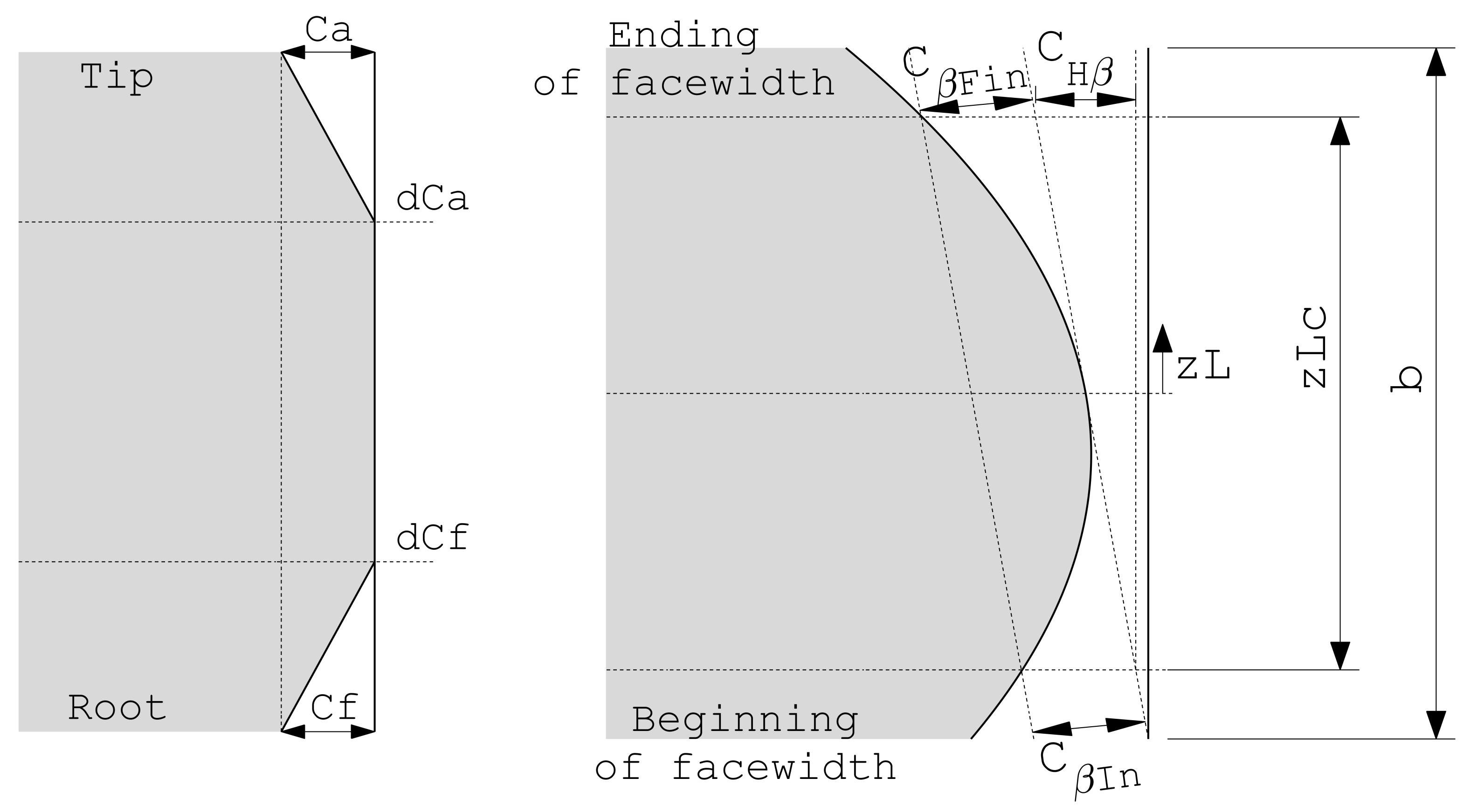
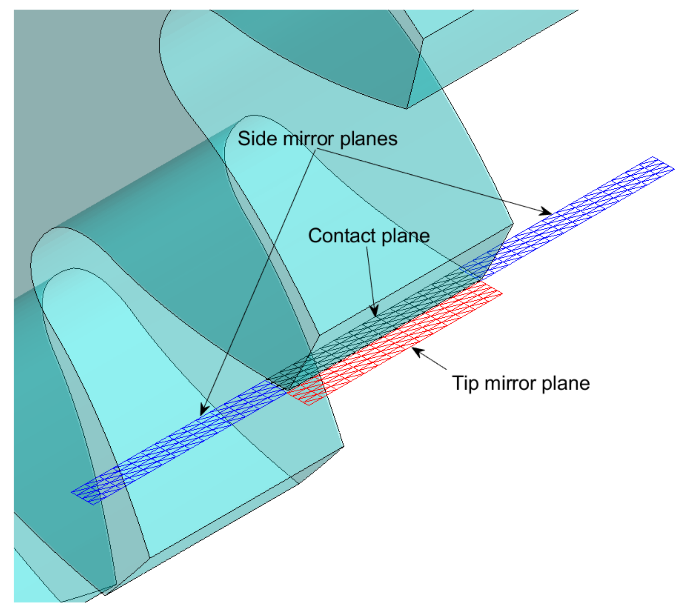
2.1. Tooth Geometry and Contact Points Detection

The detailed tooth geometry is obtained by applying Litvin’s vector approach [45] by simulating the meshing interaction between a rack cutter and the gear blank upon which TPM are then applied. Among the possible modifications along the tooth height the main ones are tip and root relief, while along the face-width crowning modifications are possible. Tip and root relief are defined by the diameter at which the modification begins ( d C a and d C f , respectively) and by the amount of material removed C a and C f , respectively, as visible in Figure 1. The amount of material removed can follow a linear law or a parabolic one. The crowning is a parabolic removal of material from the tooth face-width along its entire height. The amount of material removed at the beginning and end of the face-width is marked as C β I n and C β F i n in Figure 1 and is evaluated at a distance z L c along the face-width, while the axis of the parabola is defined by the coordinate z L . If the helix deviation C H β is different from zero, the profile of the face-width is obtained by the summation of the previously defined parabola and a further amount due to the line inclined of angle C H β .
In this work, the location of the contact point is not defined kinematically by finding the location of the intersection of the line of action (LOA) with the tooth profile at different angular positions, but it is instead sought for by a surface to surface intersection method on the rigid profiles for the first iteration, while on the deformed ones for the successive iterations of the iterative algorithm that will be described later. The surfaces of the teeth are triangulated as visible in Figure 2 and then rotated of a small angle (usually 10 5 rad) towards each other around their center of rotation and resulting intersection points are found through the application of the Möller–Trumbore ray-triangle intersection algorithm in which each triangle edge of each surface is treated as an infinitely long ray and an intersection is sought with the triangular faces of the opposite surface as visible in Figure 3 (for more details on that methodology, please refer to [44,46,47]). If an intersection is found between the ray and the surface of one of the triangles a check on the actual intersection is made by verifying if the location of the intersection point p c lies between the endpoints of the considered edge ( p 1 , p 2 ) by
| | p c p 1 | | + | | p c p 2 | | = | | p 2 p 1 | |
Usually this kind of ray tracing is computationally heavy and almost unusable without complex and specific hardware GPU acceleration, but its speed can be extremely improved by using an octree data structure [46,47] to partition the triangles in which the groups of triangles are recursively subdivided in eight bins, thus greatly reducing the computational effort by a huge amount and making it usable in an iterative process, such as the one being presented without slowing it down. Once the points of intersection between the profiles are known, the location of the contact point O = { x c p , y c p , z c p } is obtained as the average coordinates of all intersection points.

2.2. SA Deflections

Since only spur gears and no misalignment are considered in this paper, the teeth profiles are discretized in N i points at the middle of the face-width. Bending and shear properties of each tooth are computed by considering a clamped-free beam model with non-uniform geometry as by Cornell [17] instead of the integral approach of Weber [14]. By applying a load F j [id = r2] (total load exchanged by the considered flanks) the expression of deflection is
δ b i = F j c o s 2 μ α E i = 1 N i δ i l i 2 l i δ i + 1 3 δ i 2 I ¯ i + 2.4 ( 1 + ν ) + t a n 2 μ α A ¯ i
where δ i is the thickness of the i t h slice of the tooth cross-section defined by two consecutive points i and i + 1 ( i = 1 , 2 , , N i ) of the profile. E and ν are, respectively, the Young’s modulus and Poisson coefficient of the material, while A ¯ i and I ¯ i are the area and moment of inertia of the slice cross section evaluated at the middle point of the slice along tooth height, l i is the distance of the point of application of the load F j from root radius of the tooth. μ α is the working pressure angle which will be in general different from the rigid counterparts α due to teeth deflections and it is computed at the location of the contact point, as visible in Figure 4. Since all triangles considered O A B ^ , O B C ^ , O C D ^ , O D A ^ will have in general a different normal vector the average of them is found by constructing an orthogonal reference frame with origin in the contact point. Two reference frames are defined, one referred to the single triangle and, hence, a local frame (X, Y, Z) and a global one (x, y, z). The vector defining the local X axis is defined by
v x = u j O
where u j = { x j , y j , z j } and j = A , B , C , D alternatively. An accessory vector is defined by
v a = u k O
where u k = { x k , y k , z k } and k = B , C , D , A alternatively. The vectors defining the Y and Z axis are then obtained as
v z = v x × v a v y = v z × v x
The versors are then obtained dividing the vectors with their norm
n x = v x | | v x | | , n y = v y | | v y | | , n z = v z | | v z | |
Finally, the averaged versor defined with respect to the global reference frame and normal to the surface in the contact point is simply obtained by
n ¯ z = { n ¯ z , 1 , n ¯ z , 2 , n ¯ z , 3 } = { n z , OAB ^ , n z , OBC ^ , n z , OCD ^ , n z , ODA ^ } ¯
From the components of the n ¯ z versor the actual pressure angle μ α can be found by
μ α = t a n 1 n ¯ z , 2 n ¯ z , 1
Additionally, the compliance of the fillet region of the tooth and its foundation is included through an analytical expression based on the theory of elastic rings as [48,49]
δ f i = F j c o s 2 μ α b E L * u s f 2 + M * u s f + P 1 + Q t a n 2 μ α
where b is the facewidth of the gear, u is the distance between the tooth base and the point of application of the load on the tooth centerline, while s f is the chordal resisting section measured at tooth root. The coefficients L * , M * , P * , Q * are computed as
X * ( h f , i , θ f ) = A i / θ f + B i h f , i 2 + C i h f , i θ f + D i / θ f + E i h f , i + F i
where h f , i is the ratio between the root circle and hub radii, while θ f is half of the tooth root angular thickness. The coefficients A i , B i , C i , D i , E i , F i are given in Table 1. Finally, by using the superposition principle, the total deflection of a tooth pair j contacting at point i can be defined as
δ j i = δ b i p + δ f i p + δ b i g + δ f i g
where the subscript p indicates the deformation of the driving pinion, while g of the driven gear. Those deformations are computed for each point of the profiles and will later be applied to the 3D flanks in the procedure to obtain the equilibrium contact point. Hence, the total stiffness of the engaging teeth pair j contacting in point i can be expressed as
k j i = F j δ j i

2.3. Nonlinear Algorithm

As detailed in [50] during engagement the elastic deformation of the meshing teeth pairs causes a relative sliding between the contacting flanks causing a subsequent shift of the contact point where the load should be applied. Since the contact point changes, the stiffness of the engaged pair changes thus also altering the load sharing characteristics. Furthermore, due to the deflection of the gear body teeth pairs not originally in rigid contact can touch, while for the same reason the opposite might happen. For those considerations an iterative approach has been applied starting from the rigid contact conditions and then updating the contact point, the load of each teeth pair and the number of pairs in contact. At the k t h iteration using the updated contact point for the j t h pair the load sharing coefficient is computed by [51]
C k , j = k j i = 1 N k i 1 + i = 1 N k l E ˜ j l F
where E ˜ j l = δ j δ l and k j is defined in Equation (12) while F = T / r b = j = 1 N F j , where T is the total torque to be transmitted and r b is the base radius of the pinion. A natural equilibrium condition is reached when the contact points of the different engaging pairs are in a stable position, as well as the load sharing coefficients, meaning
x k , j x k 1 , j x k , j < ϵ x y k , j y k 1 , j y k , j < ϵ y z k , j z k 1 , j z k , j < ϵ z C k , j C k 1 , j C k , j < ϵ C
where x k , j , y k , j , z k , j are the coordinates of the contact point of the j t h engaging pair at the k t h iteration and ϵ x , ϵ y , ϵ z , and ϵ C are tolerance values generally equal to 10 2 % . Once equilibrium is reached a detailed contact model, described in the next paragraph, is used to study the contact between the so obtained deformed profiles.

2.4. Non-Hertzian Contact Model

To account for the continuously changing curvature of the flanks, the effects of the profile modifications and discontinuities, such as the gear edges and tip, a detailed numerical rough frictionless non-Hertzian contact model is implemented. The contact problem is usually stated as the Hertz–Signorini–Moreau problem [52,53,54]
h 0 , p n 0 , h · p n = 0 ,
The first condition enforces that no interpenetration can occur between the contact bodies and, therefore, the gap function h , which measures the distances between the surfaces, can only be positive or equal to 0 in the contact area. The second condition imposes that the contact is non-adhesive whereas the third condition enforces that the normal pressures p n can only be different from 0 inside the contact area where h = 0 and null everywhere else. The gap function h is expressed as
h = h 0 + g + δ
where h 0 is the indentation between the profiles imposed as a rigid body motion along the contact normal, g is the initial separation of the contacting surfaces and represents its topography, while δ represents the elastic deformation of the surfaces due to the applied normal pressure p n and can be expressed as [55]
δ = C · p n
where C is a matrix of the influence coefficients which introduces the elasticity of the contacting surfaces. Its components C i j ( i , j = 0 , 1 , N ) relate the displacement δ i at a point i due to the application of a unit pressure at point j were proposed by Kalker and Van Randen [56] and later fully derived and corrected by Boedo [57]. A linearly varying normal pressure p ( ξ , η ) is imposed on the half-space region as
p ξ , η = P 0 η γ
In which P 0 is the pressure in the apex ( 0 , γ ) of the triangle in the local coordinate frame ( ξ , η ) with γ > 0 as visible in Figure 5.
The displacement Equation (17) is then solved, and a closed-form solution is obtained
I ( a , b , c , t ) = ( a + b c ) ( t c ) [ ( a + b t ) 2 + ( t c ) 2 ] 1 / 2 4 π ( 1 + b ) 2 | ( t c ) | + t 2 c 2 4 π a r c s i n h a + b t t c + ( a + b c ) ( 2 c a b + b 2 c ) 4 π ( 1 + b 2 ) 3 / 2 l n ( A + B )
where
A = 2 b ( a + b t ) + 2 ( t c ) ( 1 + b 2 ) 1 / 2
B = 2 ( t c ) [ ( a + b t ) 2 + ( t c ) 2 ] 1 / 2 | t c |
While parameters a,b,c and t are dependent on the shape and size of the triangle, as described in [57]. Equation (19) is used in several limits in order obtain the displacements δ depending on the non-dimensional distance y ¯ = y / γ , since it is undefined when t = c . The dimensional pressure-displacement coefficients are obtained as
w i j , k = δ 1 ν G
where G = E 2 ( 1 + ν ) is the shear modulus of the material, E is the Young’s modulus and ν is the Poisson coefficient and k = 1 , 2 , 3 since the values of w i j , k for the entire triangulation need to be obtained three times, considering as the apex γ a different vertex of each triangle. Once this is done, the influence coefficient relating node i to node j is found by
C i j = j = 1 j = n k = 1 , 2 , 3 w i j , k
where n is the number of nodes in the triangulation and the summation is carried out by choosing the appropriate k in which node i is the vertex γ in the local coordinate frame. The process is repeated for the pinion p and the driven gear g and the final influence coefficient matrix is defined as
C = C p + C g
The surfaces displacements can then be obtained from
h s = C s p
where s = p , g . To solve the problem stated in Equation (15) and satisfy all the conditions a two nested sub-iterative processes are needed, as detailed in [50,58] to remove the residual traction stresses and to obtain the correct total transmitted force based on the computed force at the k t h iteration f k and the value at the previous one f k 1 . The first one is used to identify the correct contact footprint devoid of tension forces given a certain initial indentation h 0 , while the second is used to estimate the correct indentation to impose to the profiles so that the resulting transmitted force is within tolerance of the applied load. To validate the proposed approach and ellipsoid to ellipsoid contact is compared to the results from Hertz theory [52]. The two contacting ellipsoids ( E 1 = E 2 = 210 GPa, ν 1 = ν 2 = 0.3 ) have major radii R 1 = 100 mm and R 2 = 20 mm and minor radii r 1 = 40 mm and r 2 = 5 mm, respectively, pressed together by a normal load F = 10,500 N on a 3 × 3 mm contact plane with equilateral triangles with a side length l = 0.06 mm. The obtained pressure distribution is visible in Figure 6 in which the white line represents the predicted contact area from Hertz’s theory. The visual comparison shows a very good agreement and a numerical comparison is shown in Figure 7 where the obtained values for a varying load between 1000 ÷ 15,000 N show an error for both the maximum pressure and the contact area always lower than 1.6 % . The influence of the mesh size is also visible in the same figure for the maximum load and shows a trend quickly approaching lower errors as the length of the triangles sides decreases.
The proposed contact model has been derived from the elastic half-space theory and, hence, implies that in any transverse section a plane state of deformations is respected. However, when one or both the contacting bodies have finite length, it is evident that the end faces are to be treated as free boundaries, but in a plane state of deformations two shear stresses and a normal stress would be present at the free faces. To remove those unrealistic stresses a correction based on mirror pressure distribution and an iterative computation was proposed by Heteńyi [59,60]. However, the iterative part is time consuming as the number of iterations could theoretically go to infinity as the accuracy required increases [61] and for this reason a correction factor was proposed [62] of the form
ψ g = 1.29 1 1 ν ( 0.08 0.5 ν )
For a body a of finite length with both free ends, the influence coefficient matrix with the corrected mirroring planes is obtained as
C corr , a = C a + ψ g C mirror , left + ψ g C mirror , right
If the two bodies in contact have different finite length the mirroring operation is carried out accordingly at the free edges of each body. In order to verify the non-Hertzian results and the efficiency of the mirroring correction a model of a crowned roller bearing contacting with a cylindrical inner race has been compared with the results from [61] and the geometrical and material data are reported in Table 2. A mesh of right triangles with equal sides of 0.02 mm was defined and the resulting non-Hertzian pressure distribution obtained by the application of the current method can be seen in Figure 8 for a load F = 33,800 N where a distinct pressure peak can be distinguished at the edge of the crowned roller, while the central part has a trend similar to the ellipsoid to ellipsoid contact seen in Figure 6. The obtained results agree extremely well with the numerical and FE values detailed in [61], although minor differences are present due to the different discretization of the contact plane.

2.5. Application to Gear Contact

Since the equilibrium contact point is known through the algorithm detailed in Section 2.3, the mean tangent plane to both gear profiles is taken as the plane where contact will lie. From this line the initial separation h 0 is obtained as the normal distance between the mean common tangent at the equilibrium contact point and the deformed profiles. In the ellipsoid–ellipsoid contact, as well as the crowned roller and inner race contact shown earlier, the imposed rigid body indentation h 0 was intended as a vertical displacement of either body towards the other. In the pinion–gear contact instead, in order to respect the meshing kinematics, a rotation is imposed as a rigid body rotation of the pinion towards the gear. Therefore, at each iteration it is needed to estimate again the initial separation g k obtained through a tentative rigid body rotation θ 0 , k for the k t h iteration computed as
θ 0 , k = θ 0 , k 1 + θ 0 , k 1 θ 0 , k 2 f k f k 1 ( F j f k 1 )
Evidently also gears have finite face-width and, therefore, the mirroring operation is carried out as described earlier its effect is visible in Figure 9. The data of the tested gears are listed in Table 3 and it is clear that if no mirroring is applied two important pressure peaks are present at the free edges of the contacting flanks, which disappear as expected when the proper measures are taken. However, if one of the two bodies has a face-width greater than the other those peaks correctly reappear, although with lower values. Furthermore, gears have another free side at the tip of the tooth which must be taken into account. For this reason, a tip mirror plane is accounted for when part of the contact plane of one of the two gears lies outside of the flank and in this case the tip edge is taken as the mirror line, as visible in Figure 10.

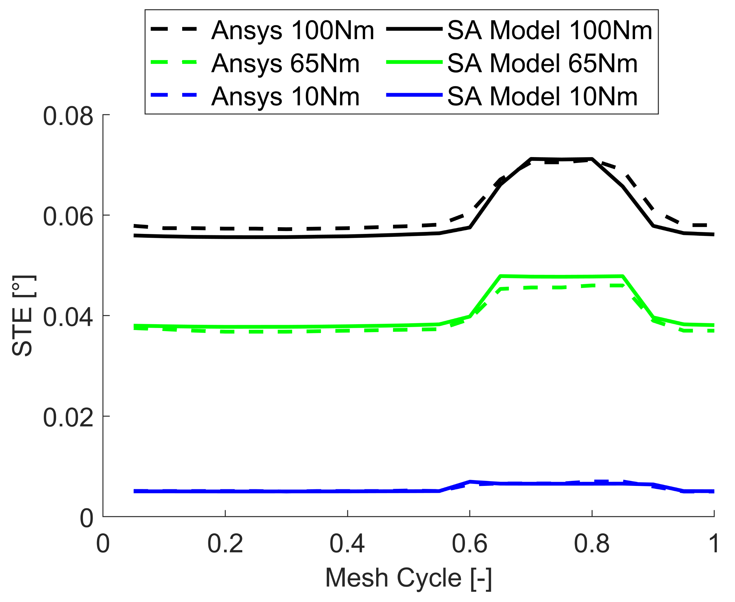
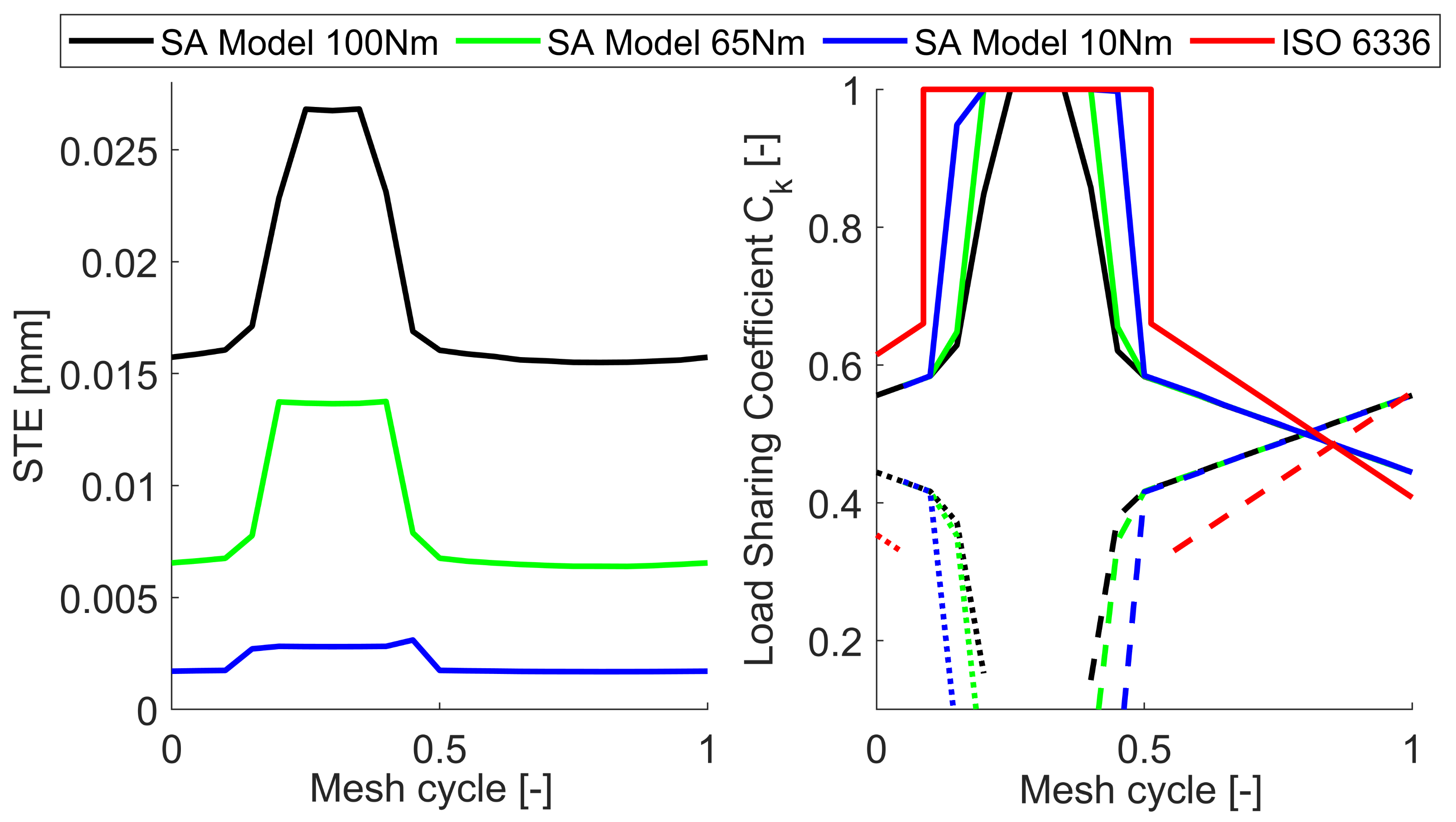
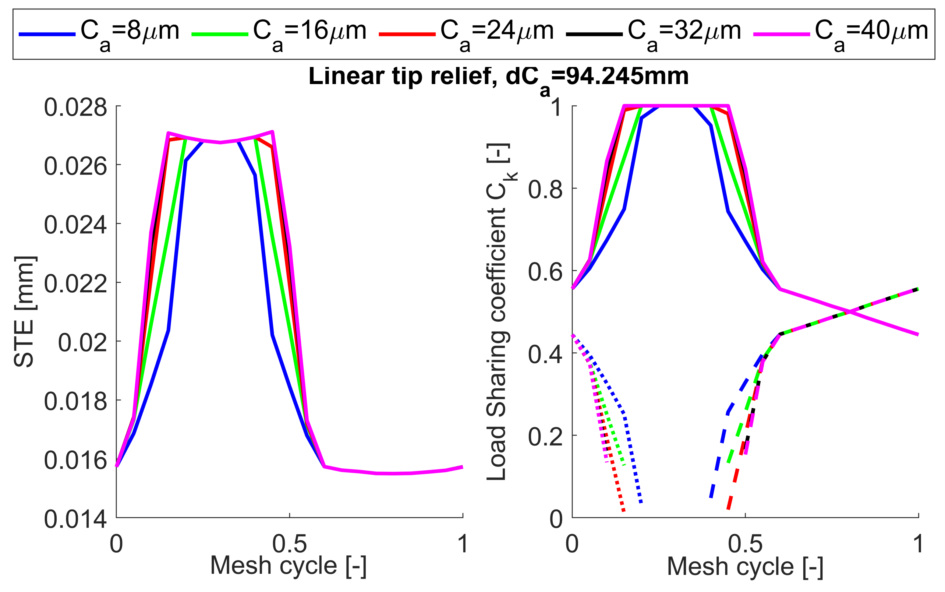
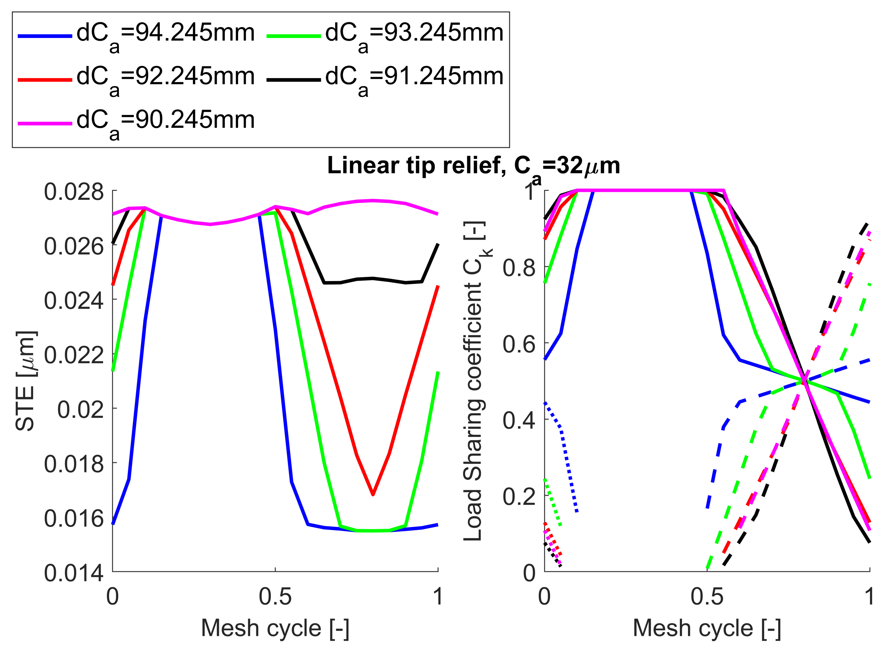
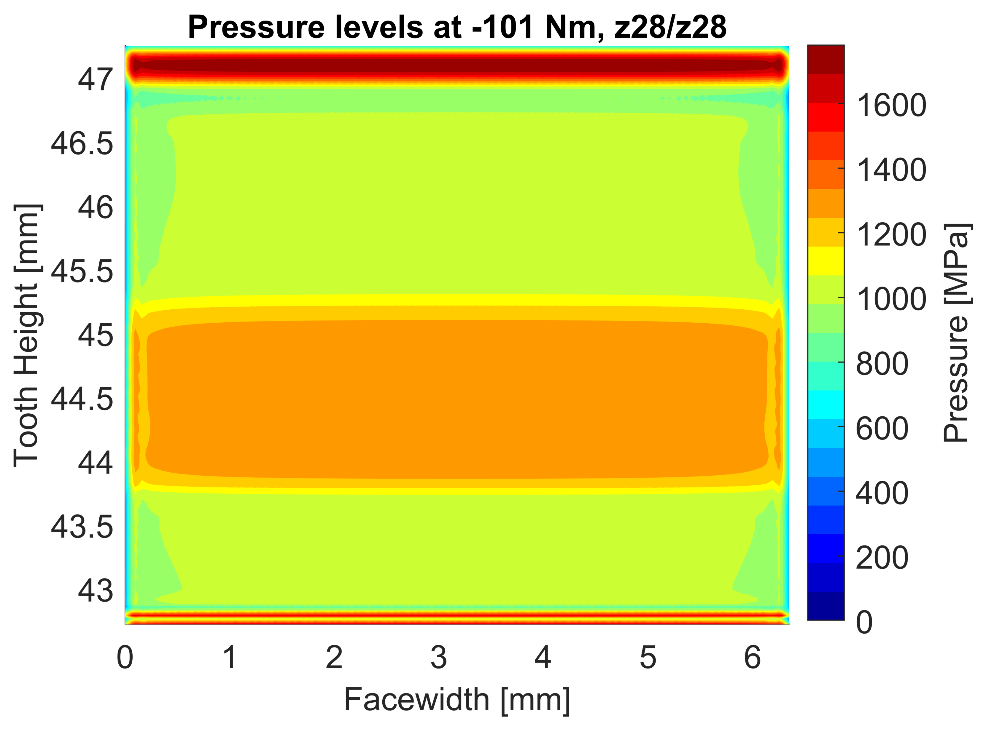
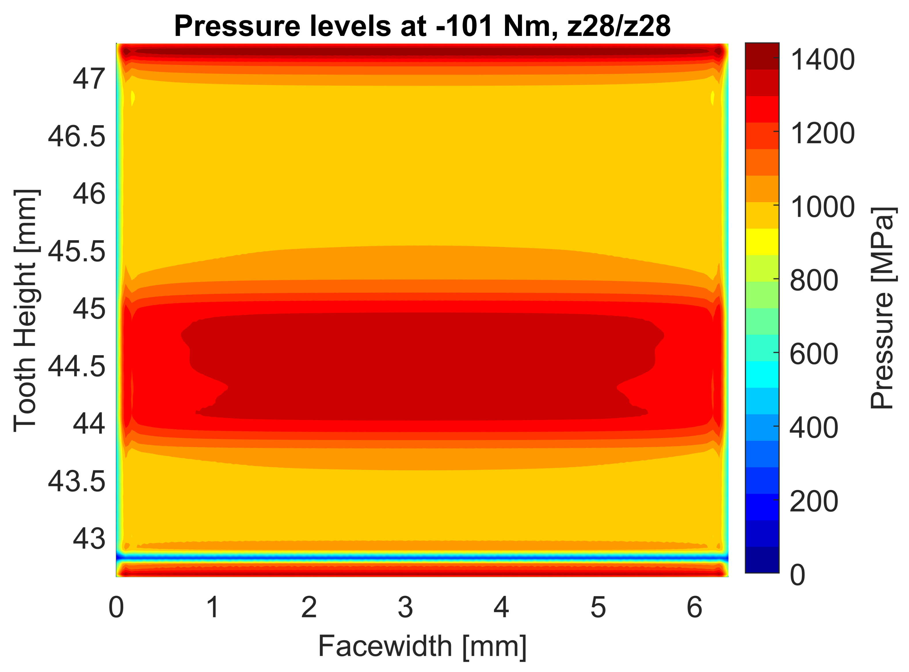
3. Application to Case Studies

The final expression for the STE, considering the cumulative effect of the SA deflections and the contact analysis, can be given as
S T E = max θ g r b , g θ p r b , p j
where the rotations of the j t h engaged pair of the pinion (p) and driven gear (g) are measured at the point of maximum displacement inside the contact area. Since the analyses in the present paper will deal with quasi-static conditions no dynamic effect is included. Additionally, no manufacturing, mounting, or other possible errors are considered at this point, hence the STE is equal to the global transmission error (TE). Results from the proposed SA approach are firstly compared against a 3D FE model from Ansys which adopts quadratic 20-node solid elements (SOLID186) and a very refined mesh ( 0.01 mm for a total of 441,562 nodes, 394,002 elements and 1,311,456 degrees of freedom) for the contacting flanks which are modeled as pairs of frictionless contact-target elements (CONTA174-TARGE170) in surface-to-surface contact using the augmented Lagrangian algorithm. The hub of the pinion gear is grounded through rigid body elements to a central node which is only free to rotate around its axis and where the torque is applied and the displacement recorded. Similarly, the hub of driven gear is constrained against all possible motion. The FE mesh and an example of the obtained contact pressures are visible in Figure 11, while the relevant data are listed in Table 3. A sequence of 20 nonlinear static analyses with automatic substepping is performed at different rotation angles to cover the whole mesh cycle which corresponds to 2 π z , as done in [63,64]. Since the transmission ratio of the studied gears is equal to one, between each analysis the FE mesh of the gears is rigidly rotated of the same angle according to their rotation directions, hence the motion is not caused by the applied torque but imposed by the angular displacement of the contacting gears. A comparison of the different approaches is visible in Figure 12 for three different torque levels. The overall agreement of the results is evident, while a small difference in the double contact zone is visible which amounts to a maximum of 0 . 002 at the highest load. The agreement is extremely good also in terms of maximum contact pressure, as visible in Figure 13, for both the single and double contact regions, as well as the pressure peaks occurring when tip-corner contact is present. However, it must be noted the the calculation in Ansys on a laptop equipped with an Intel Core i7-7700HQ CPU and 32Gb ram takes around 4 h with a so refined mesh at the surface of the engaging teeth, whereas the proposed SA approach employs only 3 min on the same machine, yielding a significant time saving without even considering the time spent to properly generate the FE model.
The STE and load sharing coefficients of the same gear pair under a load of 100 Nm are visible in Figure 14. In the same figure, it is possible to appreciate the dependency of the load sharing factor and contact ratio with respect to the torque level. In particular, it is evident that the increase in the contact ratio as the torque increases which is not considered by the standards. The actual contact ratio, which can be extracted by the load sharing characteristics, ranges from the value computed according to literature [65] 1.638 to the highest 1.85 due to the maximum torque, that corresponds to an increase of about 13%. A detailed pressure map of the flank at the highest torque displaying the pressure peaks due to tip contact is shown in Figure 15. Under these conditions the maximum pressure reaches 2648 MPa which could cause surface damage since it is higher than the design value in the single contact zone (1336 MPa).
To mitigate this problem, the effect of the linear tip relief is now analyzed. Firstly, an amount of material removed C a is analyzed for a fixed modification diameter d C a = 94.245 mm as visible in Figure 16 varying from C a = 0.008 ÷ 0.040 mm. Evidently, this modification slightly affects the mesh-in and mesh-out condition of the engaging flanks, effectively reducing the contact ratio since the single contact zone of the mesh cycle grows. Furthermore, the load sharing characteristics are not greatly affected since after a certain threshold increasing the amount of material removed effectively means reducing the working part of flanks due to a lower d N a [66], thus the curves of the STE and load sharing factor (LSF) converge to a new stable condition. Instead, modifying the length of the modification by reducing the start diameter of the modification d C a has a huge impact, as visible in Figure 17. The start of the modification is changed in the range d C a = 94.245 ÷ 90.245 mm and evident improvements are visible on both the STE and LSF. Indeed, the minimum value of the STE increases as the length of the modification increases, effectively reducing the peak to peak transmission error (PPTE), while simultaneously smoothing the transition between the single and double contact reducing the possibility of impacts on the flanks due to abrupt discontinuities. This kind of profile modification also has beneficial effects on the pressure distribution on the flanks as visible in Figure 18, where a linear tip relief was applied with C a = 0.032 mm and d C a = 94.245 mm. The contact area is reduced since the flanks are not able to come into contact up to the tip circle, but are limited by the presence of the modification. However, the pressure peak is greatly reduced, displaying a value of 1780 MPa which, while higher than the corresponding value in the single contact zone, is significantly reduced compared to the case where no TPM was applied.
Similar considerations can be applied when the amount of material removed C a is applied on a parabolic tip relief, as visible in Figure 19. Due to the fact that the removal rate is lower than the linear one, the effects of this parameter for a fixed d C a = 94.245 mm are even lower than before and can hardly benefit the transmission both in terms of STE and LSF. Indeed, the different curves are almost overlapping, showing only a minimal increase in the single contact region as expected. Additionally, increasing the length of modification has similar effects to what has been shown before as visible in Figure 20. Indeed, the PPTE decreases as the length increases and the transition of the load between the teeth pair is smoothed, but the overall effect is lower than the linear modification due to the lower removal rate of the material earlier mentioned. However, a gear pair modified with parabolic tip relief d C a = 94.245 mm and C a = 0.032 mm has significant benefits in terms of pressure distribution along the flank as visible in Figure 21. This kind of modification is even more effective at reducing the pressure peak around the tip and root regions since the transition between the pure involute and the modified portion of the tooth is smoother and the lower removal rate offers more material for the flanks to come into contact with. The maximum pressure achieved is indeed only 1426 MPa which is just 90 MPa higher than the single contact zone thus reducing any risk of potential damage.
Lastly, a combination of parabolic tip relief and face-width crowning will be discussed. The STE and LSF have been computed for different levels of symmetric crowning with C β = C β I n = C β F i n in combination with a parabolic tip relief with d C a = 94.245 mm and C a = 32 μ m and the results are visible in Figure 22. The axis of the parabola is fixed at z L = b / 2 (Figure 1), while the amount of material removed is evaluated at z L c = 0.8 b as commonly done in the industry. Since the symmetric crowning modification does not influence the mesh-in or mesh-out phases the LSF is unaffected while also the STE has minimal changes. Indeed, the only difference is the contribution of the elastic deflections δ p and δ g of the contact surface that increase since the contact are is more and more localized towards the axis of the parabola. This localization is also evident in Figure 23 where the pressures experienced by the flank are visible. Due to this effect the side edges are completely unloaded, however the pressure the gears are subjected towards b/2 are increased up to 1539 MPa in the single contact region and up to 1762 MPa in the tip and root zones. This kind of modification is indeed useful mostly when gears with different face-width need to be designed or when shafts misalignment due to deflections must be compensated, since otherwise side pressure peaks would appear as discussed earlier in Figure 9.

4. Conclusions

Aim of this paper has been to establish an accurate model to determine gear deflections under load and the contact condition that are present during meshing. For this purpose, on the basis of well established SA foundations a nonlinear iterative scheme was implemented seeking for a natural equilibrium condition between the location of the contact point, which slides due to the deflections, the load intensity, since the change in contact position alters the stiffness as well, and, ultimately, the number of the engaged teeth pairs. The contact between the deformed flanks has been studied in detail using a non-Hertzian contact model to account for the variable curvatures of the flanks, as well as the profile modifications. Appropriate measures have been included to avoid overestimations of the pressures at the free edges of the finite length gears by including a mirroring of the contact plane. A mirroring operation has also been carried out when one of the tooth tips comes in contact with the mating flank of the opposing gear. The contact model has been firstly validated against Hertz hypotheses and later for a non-Hertzian contact, giving extremely accurate results. Then, the whole proposed model has been applied to a test case and the comparison of the results against a FE counterpart has shown very good agreement. The same test case has been studied under a variety of combinations of profile modifications, namely linear and parabolic tip relief, as well as crowning. For all those tests the STE and LSF have been analyzed along with the resulting pressure distributions on the flanks of the teeth, showing different behaviors. The linear tip relief has been found to be able to effectively modify the STE and reduce the PPTE, but the parabolic one was more effective at reducing the pressure increase when contact is close to the tip of one of the gears. Indeed, the proposed SA model produces results with the same level of accuracy of a refined FE model, with some significant advantages. The setup of the model for the proposed approach is almost automatic by just specifying the parameters of the generating tool and of the wanted gear pair, while complex operations need to be carried out to set up the FE counterpart correctly. Additionally, the saving on the computational time is huge since the proposed method generates the results in minutes, while several hours are required if the FE approach is chosen instead. The present results also highlight the strong influence between the contact ratio and the applied load, the micro-geometrical modifications and the STE. A correct balance of these aspects can improve not only the endurance of the studied gears, but also their dynamic behavior. Further research will be carried out to further increase the prediction capability of this approach firstly by extending the method to model also helical gears by introducing the appropriate modifications where needed. Next, the influence of other components of the transmission such as shafts, bearings and the casing will be included to correctly estimate the contact under misaligned conditions.

Author Contributions

Conceptualization, F.B., T.M., C.M. and C.R.; methodology, F.B., T.M., C.M. and C.R; software, F.B., T.M. and C.M.; writing—original draft preparation, F.B., T.M., C.M. and C.R; writing—review and editing, F.B., T.M., C.M. and C.R. All authors have read and agreed to the published version of the manuscript.

Funding

This research received no external funding.

Data Availability Statement

The data presented in this study are available on request from the corresponding author. The data are not publicly available due to copyright issues.

Conflicts of Interest

The authors declare no conflict of interest.

Abbreviations

The following abbreviations are used in this manuscript:
STEStatic Transmission Error
SASemi Analytical
LOALine Of Action
TPMTooth Profile Modification
FEFinite Element
LSFLoad Sharing Factor

References

  1. Abersek, B.; Flasker, J.; Glodez, S. Review of mathematical and experimental models for determination of service life of gears. Eng. Fract. Mech. 2004, 71, 439–453. [Google Scholar] [CrossRef]
  2. Prasil, L.; Mackerle, J. Finite element analyses and simulations of gears and gear drives a bibliography 1997-2006. Int. J. Comput. Aided Eng. Softw. 2008, 25, 196–219. [Google Scholar] [CrossRef]
  3. Bruzzone, F.; Rosso, C. Sources of excitation and models for cylindrical gear dynamics: A review. Machines 2020, 8, 37. [Google Scholar] [CrossRef]
  4. Sato, T.; Umezawa, K.; Ishikawa, J. Effects of contact ratio and profile correction on gear rotational vibration. Bull. Jpn. Soc. Mech. Eng. 1983, 26, 2010–2016. [Google Scholar] [CrossRef] [Green Version]
  5. Umezawa, K.; Sato, T.; Ishikawa, J. Simulation on rotational vibration of spur gears. Bull. Jpn. Soc. Mech. Eng. 1984, 27, 102–109. [Google Scholar] [CrossRef] [Green Version]
  6. Umezawa, K.; Ajima, T.; Houhoh, H. Vibration of three axes gear system (in Japanese). Bull. Jpn. Soc. Mech. Eng. 1986, 29, 950–957. [Google Scholar] [CrossRef] [Green Version]
  7. Kubo, A.; Kiyono, S.; Fujino, M. On analysis and prediction of machine vibration caused by gear meshing (1st report, nature of gear vibration and the total vibrational excitation). Bull. Jpn. Soc. Mech. Eng. 1986, 29, 4424–4429. [Google Scholar] [CrossRef]
  8. Yang, D.C.H.; Lin, J.Y. Hertzian damping, tooth friction and bending elasticity in gear impact dynamics. Trans. Am. Soc. Mech. Eng. J. Mech. Transm. Autom. Des. 1986, 109, 189–196. [Google Scholar] [CrossRef]
  9. Ozguven, H.N.; Houser, D.R. Mathematical models used in gear dynamics—A review. J. Sound Vib. 1988, 121, 383–411. [Google Scholar] [CrossRef]
  10. Kadmiri, Y.; Perret-Liaudet, J.; Rigaud, E.; Le Bot, A.; Vary, L. Influence ofmultiharmonics excitation on rattle noise in automotive gearboxes. Adv. Acoust. Vib. 2011, 2011, 659797. [Google Scholar]
  11. Bel Mabrouk, I.; El Hami, A.; Walha, L.; Zghal, B. Dynamic vibrations in wind energy systems: Application to vertical axis wind turbine. Mech. Syst. Signal Process. 2017, 85, 396–414. [Google Scholar] [CrossRef]
  12. Garambois, P.; Donnard, G.; Rigaud, E.; Perret-Liaudet, J. Multiphysics coupling between periodic gear mesh excitation and input/output fluctuating torques: Application to a roots vacuum pump. J. Sound Vib. 2017, 405, 158–174. [Google Scholar] [CrossRef] [Green Version]
  13. Harris, S.L. Dynamic loads on teeth of spur gears. Proc. Inst. Mech. Eng. 1958, 172, 87–112. [Google Scholar] [CrossRef]
  14. Weber, C. The Deformation of Load Gears and the Effect on Their Load-Carrying Capacity; Technical Report n.3; British Department of Scientific and Industrial Research: London, UK, 1949. [Google Scholar]
  15. Weber, C.; Banaschek, K. Formänderung und Profilrücknahme bei Gerad-und Schragverzahnten Antriebstechnik; Vieweg: Braunschweig, Germany, 1953. [Google Scholar]
  16. Cornell, R.W.; Westervelt, W.W. Dynamic tooth loads and stressing for high contact ratio spur gears. Trans. Am. Soc. Mech. Eng. J. Mech. Des. 1978, 100, 69–76. [Google Scholar] [CrossRef]
  17. Cornell, R.W. Compliance and stress sensitivity of spur gear teeth. J. Mech. Des. 1981, 103, 447–459. [Google Scholar] [CrossRef] [Green Version]
  18. Ishikawa, J. Fundamental investigations on the design of spur gears. Bull. Tokyo Inst. Technol. 1957, 197, 55–62. [Google Scholar]
  19. Cai, Y.; Hayashi, T. The optimum modification of tooth profile of power transmission spur gears to make the rotational vibration equal zero. Trans. Jpn. Soc. Mech. Eng. 1991, 57, 3957–3963. [Google Scholar] [CrossRef] [Green Version]
  20. Cai, Y.; Hayashi, T. The linear approximated equation of vibration of a pair of spur gears. J. Mech. Des. 1994, 116, 558–564. [Google Scholar] [CrossRef]
  21. Chi, C.W.; Howard, I.; Wang, J.D. An Experimental Investigation of the Static Transmission Error and Torsional Mesh Stiffness of Nylon Gears. In Proceedings of the 10th International Power Transmission and Gearing Conference, Las Vegas, ND, USA, 4–7 September 2007; Volume 7, pp. 207–216. [Google Scholar]
  22. Raghuwanshi, N.K.; Parey, A. Experimental measurement of gear mesh stiffness of cracked spur gear by strain gauge technique. Measurement 2016, 86, 266–275. [Google Scholar] [CrossRef]
  23. Raghuwanshi, N.K.; Parey, A. Experimental measurement of mesh stiffness by laser displacement sensor technique. Measurement 2018, 128, 63–70. [Google Scholar] [CrossRef]
  24. Wei, J.; Sun, W.; Wang, L. Effect of flank deviation on load distributions for helical gear. J. Mech. Sci. Technol. 2011, 25, 1781–1789. [Google Scholar] [CrossRef]
  25. Zhang, Y.; Wang, Q.; Ma, H.; Huang, J.; Zhao, C. Dynamic analysis of three-dimensional helical geared rotor system with geometric eccentricity. J. Mech. Sci. Technol. 2013, 27, 3231–3242. [Google Scholar] [CrossRef]
  26. Inalpolat, M.; Handschuh, M.; Kahraman, A. Influence of indexing errors on dynamic response of spur gear pairs. Mech. Syst. Signal Process. 2015, 60–61, 391–405. [Google Scholar] [CrossRef]
  27. Wang, Q.; Zhang, Y. A model for analyzing stiffness and stress in a helical gear pair with tooth profile errors. J. Vib. Control 2017, 23, 272–289. [Google Scholar] [CrossRef]
  28. Deng, G.; Nakanishi, T.; Inoue, K. Bending load capacity enhancement using an asymmetric tooth profile. JSME Int. J. Ser. C 2003, 46, 1171–1177. [Google Scholar] [CrossRef] [Green Version]
  29. Lin, T.; Ou, H.; Li, R. A finite element method for 3D static and dynamic contact/impact analysis of gear drives. Comput. Methods Appl. Mech. Eng. 2007, 196, 1716–1728. [Google Scholar] [CrossRef]
  30. Pedersen, N.L.; Jorgenses, M.F. On gear tooth stiffness evaluation. Comput. Struct. 2014, 135, 109–117. [Google Scholar] [CrossRef]
  31. Ural, A.; Heber, G.; Wawrzynek, P.A.; Ingraffea, A.R.; Lewicki, D.G.; Neto, J.B. Three-dimensional, parallel, finite element simulation of fatigue crack growth in a spiral bevel pinion gear. Eng. Fract. Mech. 2005, 72, 1148–1170. [Google Scholar] [CrossRef]
  32. Chaari, F.; Fakhfakh, T.; Haddar, M. Analytical modelling of spur gear tooth crack and influence on gearmesh stiffness. Eur. J. Mech.-A/Solids 2009, 28, 461–468. [Google Scholar] [CrossRef]
  33. Qin, W.; Guan, C. An investigation of contact stresses and crack initiation in spur gears based on finite element dynamics analysis. Int. J. Mech. Sci. 2014, 83, 96–103. [Google Scholar] [CrossRef]
  34. Curà, F.; Mura, A.; Rosso, C. Effect of rim and web interaction on crack propagation paths in gears by means of XFEM technique. Fatigue Fract. Eng. Mater. Struct. 2015, 38, 1237–1245. [Google Scholar] [CrossRef]
  35. Cura, F.; Mura, A.; Rosso, C. Investigation about crack propagation paths in thin rim gears. Frat. Integrita Strutt. 2014, 30, 446–453. [Google Scholar] [CrossRef] [Green Version]
  36. Hertz, H.R. On contact between elastic bodies. Collect. Works 1895, 1, 155–173. [Google Scholar]
  37. Hu, W.; Chen, Z. A multi-mesh mpm for simulating the meshing process of spur gears. Comput. Struct. 2003, 81, 1991–2002. [Google Scholar] [CrossRef]
  38. Wang, J.D.; Howard, I.M. Error analysis of finite element modeling of involute spur gears. J. Mech. Des. 2006, 128, 90–97. [Google Scholar] [CrossRef]
  39. He, S.; Gunda, R.; Singh, R. Effect of sliding friction on the dynamics of spur gear pair with realistic time-varying stiffness. J. Sound Vib. 2007, 301, 927–949. [Google Scholar] [CrossRef]
  40. Tesfahuneng, Y.A.; Rosa, F.; Gorca, C. The effects of the shape of tooth profile modifications on the transmission error, bending and contact stress of spur gears. Proc. Inst. Mech. Eng. Part C J. Mech. Eng. Sci. 2010, 224, 1749–1758. [Google Scholar] [CrossRef]
  41. Nikolic, V.; Dolicanin, C.; Dimitrijevic, D. Dynamic model for the stress and strain state analysis of a spur gear transmission. J. Mech. Eng. 2012, 58, 56–67. [Google Scholar] [CrossRef]
  42. Creţu, S.S.; Pop, N.N.; Cazan, S.V. Considerations regarding the pressures distribution on leads of spur gears. IOP Conf. Ser. Mater. Sci. Eng. 2018, 444, 022022. [Google Scholar] [CrossRef]
  43. Parker, R.G.; Vijayakar, S.M.; Imajo, T. Non-linear dynamic response of a spur gear pair: Modelling and experimental comparisons. J. Sound Vib. 2000, 237, 435–455. [Google Scholar] [CrossRef] [Green Version]
  44. Möller, T.; Trumbore, B. Fast. minimum storage ray-triangle intersection. J. Graph. Tools 1997, 2, 21–28. [Google Scholar] [CrossRef]
  45. Litvin, F.L. Gear Geometry and Applied Theory; P. T. R. Prentice Hall: Hoboken, NJ, USA, 1994. [Google Scholar]
  46. Meagher, D. Octree Encoding: A New Technique for the Representation, Manipulation and Display of Arbitrary 3-D Objects by Computer; Technical Report IPL-TR-80-111; Rensselaer Polytechnic Institute: Rensselaer County, NY, USA, 1980. [Google Scholar]
  47. Fast Mesh-Mesh Intersection Using Ray-Tri Intersection with Octree Spatial Partitioning. Available online: https://jp.mathworks.com/matlabcentral/fileexchange/49160-fast-mesh-mesh-intersection-using-ray-tri-intersection-with-octree-spatial-partitioning (accessed on 12 September 2019).
  48. Muskhelishvili, N. Some Basic Problems of the Mathematical Theory of Elasticity; P. Noordhoff Limited: Groningen, The Netherlands, 1975. [Google Scholar]
  49. Sainsot, P.; Velex, P.; Duverger, O. Contribution of gear body to tooth deflections - A new bidimensional analytical formula. J. Mech. Des. 2004, 126, 748–752. [Google Scholar] [CrossRef]
  50. Bruzzone, F.; Maggi, T.; Marcellini, C.; Rosso, C. 2D Nonlinear and non-Hertzian gear teeth deflection model for static transmission error calculation. Mech. Mach. Theory 2021, 166, 104471. [Google Scholar] [CrossRef]
  51. Ma, H.; Pang, X.; Feng, R.J.; Zeng, J.; Wen, B.C. Improved time-varying mesh stiffness model of cracked spur gears. Eng. Fail. Anal. 2015, 55, 271–287. [Google Scholar] [CrossRef]
  52. Johnson, K.L. Contact Mechanics; Cambridge University Press: Cambridge, MA, USA, 1985. [Google Scholar]
  53. Kalker, J.J. Three-Dimensional Elastic Bodies in Rolling Contact; Springer: Dordrecht, The Netherlands, 1990. [Google Scholar]
  54. Wriggers, P. Computational Contact Mechanics; Springer: Berlin/Heidelberg, Germany, 2002. [Google Scholar]
  55. Sayles, R.S. Basic principles of rough surface contact analysis using numerical methods. Tribol. Int. 1996, 29, 639–650. [Google Scholar] [CrossRef]
  56. Kalker, J.J.; Randen, Y.V. A minimum principle for frictionless elastic contact with application to non-Hertzian half-space contact problems. J. Eng. Math. 1972, 6, 193–206. [Google Scholar] [CrossRef]
  57. Boedo, S. A corrected displacement solution to linearly varying surface pressure over a triangular region on the elastic half-space. Tribol. Int. 2013, 60, 116–118. [Google Scholar] [CrossRef]
  58. Marmo, F.; Rosati, L. A general approach to the solution of Boussinesq’s problem for polynomial pressures acting over polygonal domains. J. Elast. 2016, 122, 75–112. [Google Scholar] [CrossRef]
  59. Heteńyi, M. A Method of Solution for the Elastic Quarter-Plane. J. Appl. Mech. 1960, 82, 289–296. [Google Scholar] [CrossRef]
  60. Heteńyi, M. A General Solution for the Elastic Quarter Space. J. Appl. Mech. 1970, 37, 70–76. [Google Scholar] [CrossRef]
  61. de Mul, J.M.; Kalker, J.J.; Fredriksson, B. The contact between arbitrarily curved bodies of finite dimensions. J. Tribol. 1986, 108, 140–148. [Google Scholar] [CrossRef]
  62. Guilbault, R. A fast correction for elastic quarter-space applied to 3D modelling of edge contact problems. J. Tribol. 2011, 133, 031402. [Google Scholar] [CrossRef]
  63. Jabbour, T.; Asmar, G. Tooth stress calculation of metal spur and helical gears. Mech. Mach. Theory 2015, 92, 375–390. [Google Scholar] [CrossRef]
  64. Zhan, J.; Fard, M.; Jazar, R. A quasi-static FEM for estimating gear load capacity. Measurement 2015, 75, 40–49. [Google Scholar] [CrossRef]
  65. ISO 6336-1:2019. Calculation of Load Capacity of Spur and Helical Gears; International Organization for Standardization: Geneva, Switzerland, 2019. [Google Scholar]
  66. ISO 21771-1:2007. Gears—Cylindrical Involute Gears and Gear Pairs—Concepts and Geometry; International Organization for Standardization: Geneva, Switzerland, 2007. [Google Scholar]
Figure 1. Nomenclature of different TPM. (left) Tip and root relief modifications, (right) TPM along the face-width.
Machines 09 00223 g001
Figure 2. Triangulated tooth surfaces in initial rigid contact.
Machines 09 00223 g002
Figure 3. Surface intersection between two engaging teeth and location of the contact point at equilibrium after deformation.
Machines 09 00223 g003
Figure 4. Points considered for the calculation of the normal vector to the contact point.
Machines 09 00223 g004
Figure 5. Local reference system for the contact formulation.
Machines 09 00223 g005
Figure 6. Pressure distribution for the ellipsoid–ellipsoid contact.
Machines 09 00223 g006
Figure 7. Ellipsoid–ellipsoid contact percent error versus Hertz’s theory.
Machines 09 00223 g007
Figure 8. Pressure distributions for the crowned roller and inner race contact.
Machines 09 00223 g008
Figure 9. Effect of plane mirroring on the pressure distribution for meshing gears. (a) No mirroring, b p = b g (b) Mirroring, b p = b g (c) Mirroring, b p = 2 b g .
Machines 09 00223 g009
Figure 10. Side and tip mirror planes in gear contact used to obtain the mirror pressure distributions in order to take into account the free edges of the contacting bodies.
Machines 09 00223 g010
Figure 11. Mesh of the solid model and pressure results from Ansys.
Machines 09 00223 g011
Figure 12. Comparison of the STE obtained from the SA model and Ansys.
Machines 09 00223 g012
Figure 13. Comparison of the maximum pressure obtained from the SA model and Ansys.
Machines 09 00223 g013
Figure 14. STE and LSF of the tested gear pair without modifications.
Machines 09 00223 g014
Figure 15. Flank pressure distribution of the tested gear pair without modifications.
Machines 09 00223 g015
Figure 16. Effect of linear tip relief amount of material removed on the STE and load sharing.
Machines 09 00223 g016
Figure 17. Effect of linear tip relief length of modification on the STE and load sharing.
Machines 09 00223 g017
Figure 18. Flank pressure distribution of the tested gear pair with linear tip relief, d C a = 94.245 mm and C a = 32 μ m.
Machines 09 00223 g018
Figure 19. Effect of parabolic tip relief amount of material removed on the STE and load sharing.
Machines 09 00223 g019
Figure 20. Effect of parabolic tip relief length of modification on the STE and load sharing.
Machines 09 00223 g020
Figure 21. Flank pressure distribution of the tested gear pair with parabolic tip relief, dCa = 94.245 mm and Ca = 32 μ m.
Machines 09 00223 g021
Figure 22. Effect of parabolic tip relief length of modification on the STE and load sharing in combination with face-width crowning C β = C β I n = C β F i n , z L = b / 2 and z L c = 0.8 b ( d C a = 94.245 mm and C a = 32 μ m).
Machines 09 00223 g022
Figure 23. Flank pressure distribution of the tested gear pair with parabolic tip relief, d C a = 94.245 mm and C a = 32 μ m and C β = C β I n = C β F i n = 2 μ m, z L = b / 2 and z L c = 0.8 b parabolic crowning.
Machines 09 00223 g023
Table 1. Polynomial coefficients for Equation (10).
A i B i C i D i E i F i
L * 5.547 × 10 5 1.9986 × 10 3 2.3015 × 10 4 4.7702 × 10 3 0.02716.8045
M * 60.111 × 10 5 28.100 × 10 3 83.431 × 10 4 9.9256 × 10 3 0.16240.9086
P * 50.952 × 10 5 185.50 × 10 3 0.05380 × 10 4 5.300 × 10 3 0.28950.9236
Q * 6.2042 × 10 5 9.0889 × 10 3 4.0964 × 10 4 7.8267 × 10 3 −0.14720.6904
Table 2. Crowned roller and inner race geometrical and material properties, from [61].
Crowned Roller
Diameter d 1 15 mm
Crowning radius r 1 1114 mm
Fillet radius f 1 1.006 mm
Width b 1 16 mm
Shear modulus G 1 79.3 GPa
Poisson ratio ν 1 0.3
Inner race
Diameter d 2 58.5 mm
Width b 2 25 mm
Shear modulus G 2 79.3 GPa
Poisson ratio ν 2 0.3
Table 3. Gear pair parameters.
ParameterPinion pGear g
Number of teeth z [-]2828
Module m [mm]3.1753.175
Pressure angle α p [ ]2020
Facewidth b [mm]6.356.35
Hub radius [mm]2020
Young modulus E [MPa]210,000210,000
Poisson coefficient ν [-]0.30.3
Publisher’s Note: MDPI stays neutral with regard to jurisdictional claims in published maps and institutional affiliations.

