
Vibrodiagnostics Faults Classification for the Safety Enhancement of Industrial Machinery

 , , , , , and
Abstract
:1. Introduction
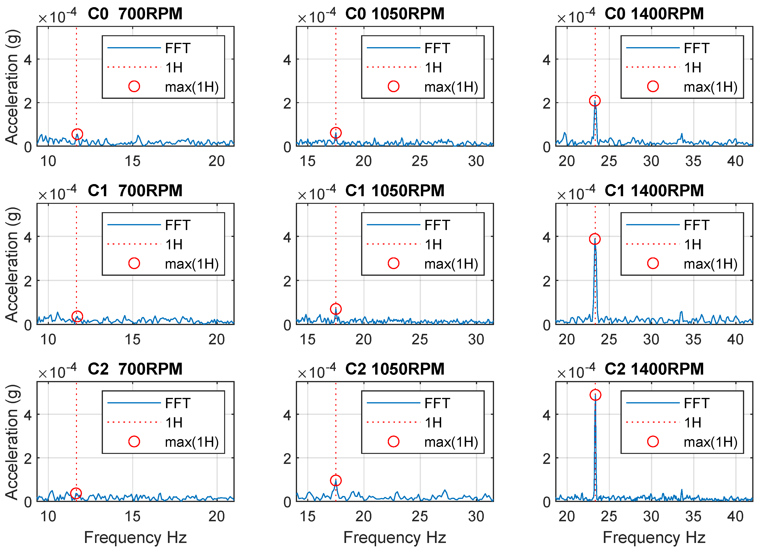
- Verify that the missing insert on the tool is detectable on the vibrodiagnostic signal measured on the machine spindle.
- Select and compare predictors from time and frequency domains.
- Effect spindle speeds on the classification success rate.
- Select and compare the most successful classification methods
- Evaluate detection success rate of fault-free state
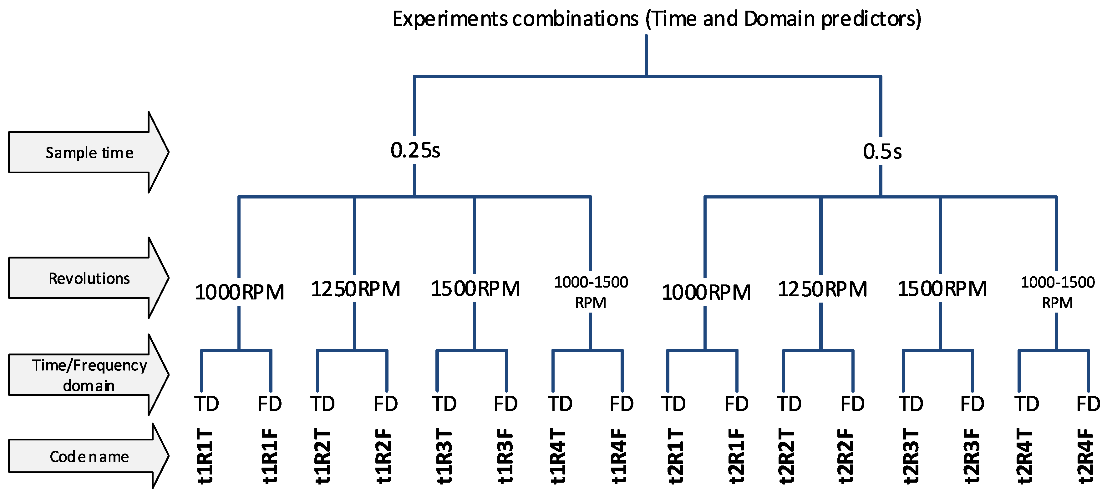
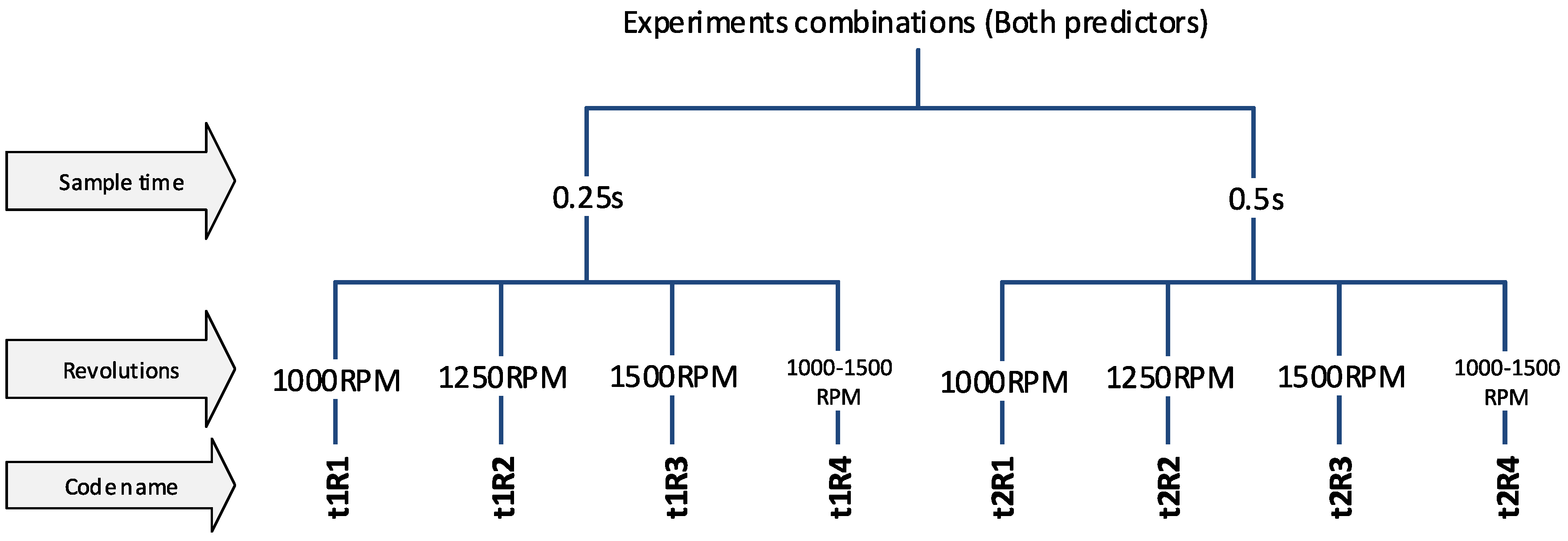
2. Experimental Procedure
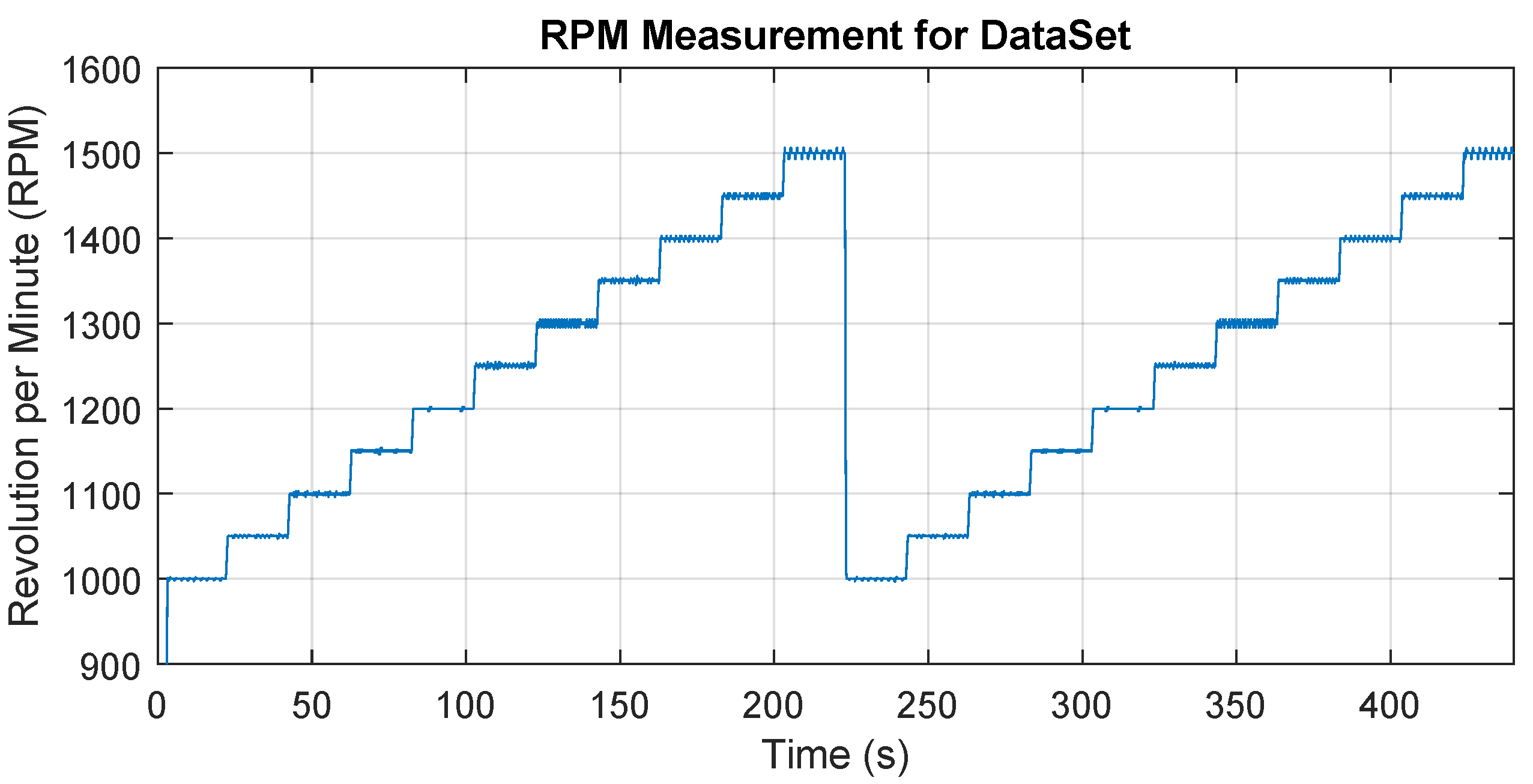
2.1. Dataset Obtain
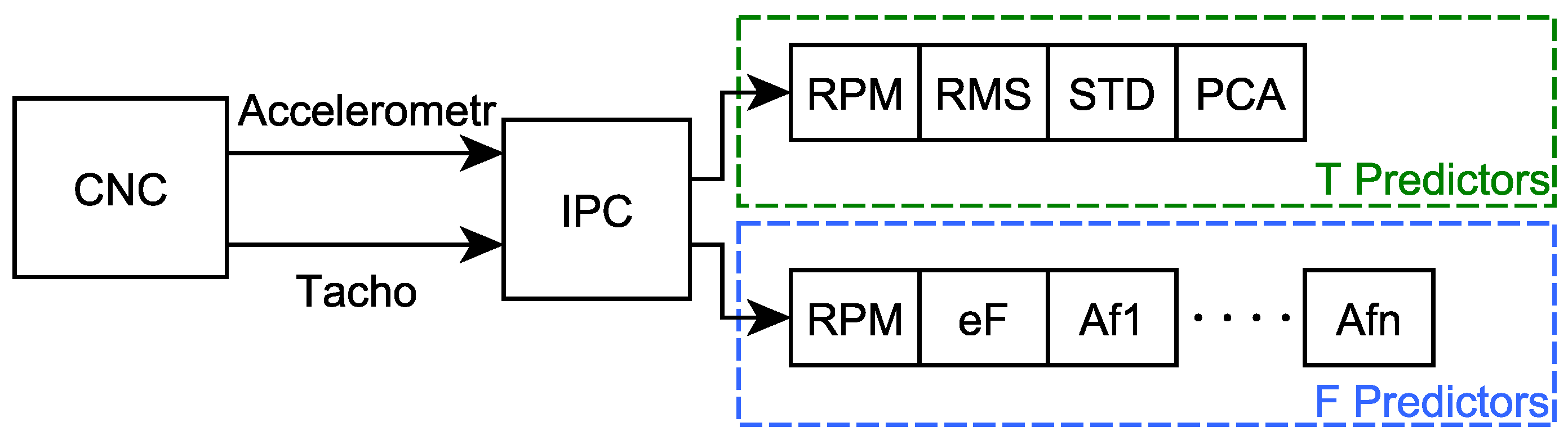
2.2. Predictors
- Clearly describe the class properties (state)-improved achievement classification
- Low computational complexity-speeds up the predictor calculation
- Low number of predictors-speeds up the learning and evaluation process
2.3. Data Processing and Selection of Predictors
- Speed-Current RPM during one sample
- RMS-Root Mean Square of acceleration amplitudes from one sample
- STD-The standard deviation of the acceleration amplitudes from a single sample
- PCA-Principal Component Analysis realized with scikit learn library R2 (with parameters n_components = 1 and explained_variance_ = 0) [22]
- Speed-Current RPM during one sample
- Spectrum energy (eF)-calculated as for the 4–100 Hz range, where are amplitudes of spectral lines.
- Af(i)-the sequence of amplitudes of individual spectral lines for frequencies 4–100 Hz
- Combination of vibration channel and tacho channel data
- Splitting the signal according to the selected time (t1 = 0.25 s or t2 = 0.5 s)
- Checking whether the change is not greater than 10 RPM during the duration (t1 or t2) (elimination of transients)
- Sorting the signal into individual classes
- Predictor calculation, for each sample (T-time domain, F-Frequency domain or FT-all predictors)
- Saving predictors to a file according to individual classes (preparation for MATLAB)
- Random mixing and merging of data of individual classes into one dataset
- Evaluating in the environment “Classification learner app”
- Generating and saving the most successful model
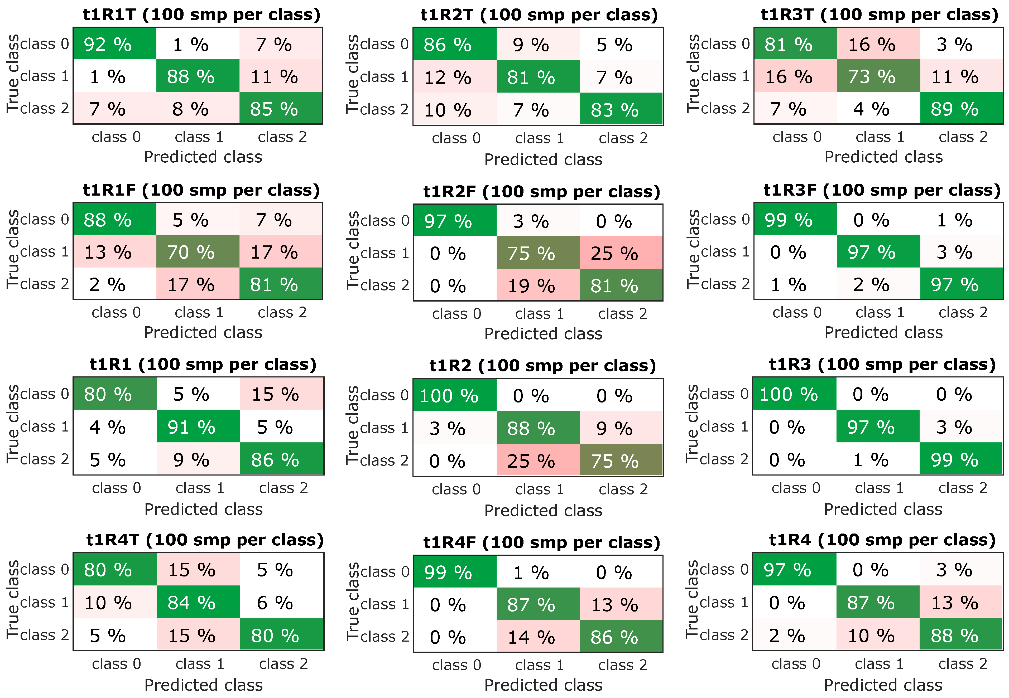
- Randomly selected n samples from each class (selected n = 100 per class)
- Accuracy and TPR (True positive rate) and FNR (False negative rate) evaluated
- Results displayed and saved as the Confusion matrix
3. Classification Methods
3.1. Classification Trees
- Fine tree
- Medium tree
- Coarse tree
3.2. Discriminant Analysis
- Linear discriminant
- Quadratic discriminant
3.3. Naive Bayes
- Gaussian Naive Bayes
- Kernel Naive Bayes
3.4. Support Vector Machine Classification
- Linear SVM
- Quadratic SVM
- Cubic SVM
- Fine Gaussian SVM
- Medium Gaussian SVM
- Coarse Gaussian SVM
3.5. Nearest Neighbors
- Fine KNN
- Medium KNN
- Coarse KNN
- Cosine KNN
- Cubic KNN
- Weighted KNN
3.6. Classification Ensembles
- Boosted Trees
- Bagged Trees
- Subspace Discriminant
- Subspace KNN
- RUSBoosted Trees
4. Comparison of Classification Results
5. Verification of Resulting Models
Time Consumption of Prediction
6. Implementation of the Trained Model
- (a)
- Data acquisition and learning process
- The server requests data from individual IPCs and creates a dataset for creating a classification model (Data is predictors-it evaluates IPCs, only predictors are transmitted).
- If there is a sufficient amount of data (or conditions have changed, etc.), then MATLAB performs learning and creates a trained classification model for a specific IPC and exports it to the C language (this MATLAB allows).
- The trained model is sent to a specific IPC.
- (b)
- Evaluation process
- IPC performs data collection and predictor calculation-this is a simple operation and can be performed in any programming language, for simplicity and availability Python was chosen, which performs statistical operations and frequency analysis.
- Performs classification using MATLAB created and trained model, which was exported to C language (Python allows to run code in C language).
7. Results and Discussions
8. Conclusions
Author Contributions
Funding
Conflicts of Interest
References
- Oravec, M.; Pacaiova, H.; Izarikova, G.; Hovanec, M. Magnetic Field Image-Source of Information for Action Causality. In Proceedings of the 2019 IEEE 17th World Symposium on Applied Machine Intelligence and Informatics (SAMI), Herl’any, Slovakia, 24–26 January 2019; pp. 101–105, ISBN 978-1-7281-0250-4. [Google Scholar]
- ISO 12100:2010. Safety of Machinery—General Principles for Design—Risk Assessment and Risk Reduction; ISO: Genova, Switzerland, 2010. [Google Scholar]
- ISO 9001:2008. Quality Management Systems; ISO: Genova, Switzerland, 2008. [Google Scholar]
- ISO 31010:2019. Risk Management—Risk Assessment Techniques; IEC: Genova, Switzerland, 2019. [Google Scholar]
- ISO 3534-1:2006. Statistics—Vocabulary and Symbols—Part 1: General Statistical Terms and Terms Used in Probability; ISO: Genova, Switzerland, 2006. [Google Scholar]
- Zuth, D.; Marada, T. Using artificial intelligence to determine the type of rotary machine fault. Mendel 2018, 24, 49–54. [Google Scholar] [CrossRef]
- Zuth, D.; Marada, T. Utilization of machine learning in vibrodiagnostics. Adv. Intell. Syst. Comput. 2018. [Google Scholar] [CrossRef]
- Zuth, D.; Marada, T. Comparison of Faults Classification in Vibrodiagnostics from Time and Frequency Domain Data. In Proceedings of the 2018 18th International Conference on Mechatronics-Mechatronika, Brno, Czech Republic, 5–7 December 2018; Volume 18, pp. 482–487, ISBN 978-802145544-3. [Google Scholar]
- Ympa, A. Learning Methods for Machine Vibration Analysis and Health Monitoring. Ph.D. Dissertation, Delft University of Technology, Delft, The Netherlands, 2001. [Google Scholar]
- Maluf, D.A.; Daneshmend, L. Application of machine learning for machine monitoring and diagnosis. Fla. Artif. Intell. Res. Symp. 1997, 10, 232–236. [Google Scholar]
- Li, C.; Sánchez, R.V.; Zurita, G.; Cerrada, M.; Cabrera, D. Fault Diagnosis for Rotating Machinery Using Vibration Measurement Deep Statistical Feature Learning. Sensors 2016, 16, 895. [Google Scholar] [CrossRef] [PubMed] [Green Version]
- Chen, Z.; Chen, X.; Li, C.; Sanchez, R.V.; Qin, H. Vibration-based gearbox fault diagnosis using deep neural networks. J. Vibroeng. 2017, 19, 2475–2496. [Google Scholar] [CrossRef]
- Popiołek, K. Diagnosing the technical condition of planetary gearbox using the artificial neural network based on analysis of non-stationary signals. Diagnostyka 2016, 17, 57–64. [Google Scholar]
- Haedong, J.; Park, S.; Woo, S.; Lee, S. Rotating Machinery Diagnostics Using Deep Learning on Orbit Plot Images. Procedia Manuf. 2016, 5, 1107–1118. [Google Scholar] [CrossRef] [Green Version]
- Scikit-Learn: Machine Learning in Python. Available online: https://scikit-learn.org/stable/index.html (accessed on 6 January 2018).
- Pánek, D.; Orosz, T.; Karban, P. Artap: Robust Design Optimization Framework for Engineering Applications. In Proceedings of the 2019 Third International Conference on Intelligent Computing in Data Sciences (ICDS), Marrakech, Morocco, 28–30 October 2019; pp. 1–6. [Google Scholar] [CrossRef] [Green Version]
- Train Models to Classify Data Using Supervised Machine Learning. MathWorks-Makers of MATLAB and Simulink. Available online: https://www.mathworks.com/help/stats/classificationlearner-app.html (accessed on 20 April 2018).
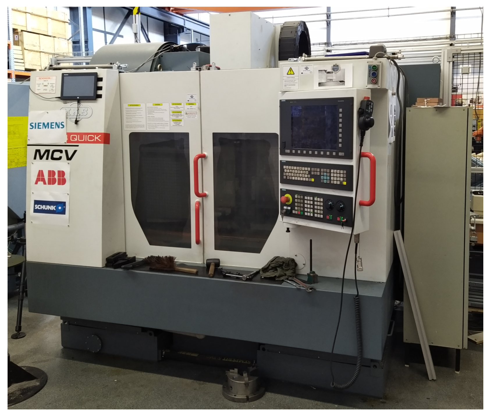
- MCV 750 | KOVOSVIT MAS. Machine tools, CNC machines, CNC lathes | KOVOSVIT MAS [online]. Copyright© KOVOSVIT MAS 2016. Available online: https://www.kovosvit.com/mcv-750-p7.html (accessed on 20 April 2018).
- Broch, J.T. Mechanical Vibration and Shock Measurements, 2nd ed.; Bruel & Kjaer: Nellum, Denmark, 1980; ISBN 978-8787355346. [Google Scholar]
- Blata, J.; Juraszek, J. Metody Technické Diagnostiky, Teorie a Praxe. Metody Diagnostyki Technicznej, Teoria i Praktika; Repronis: Ostrava, Czech Republic, 2013; ISBN 978-80-248-2997-5. [Google Scholar]
- Zuth, D.; Vdoleček, F. Měření vibrací ve vibrodiagnostice. In Automa; FCC Public: Praha, Czech Republic, 2010; pp. 32–36. ISSN 1210-9592. [Google Scholar]
- Scikit-Learn 0.23.1 Documentation. Scikit-Learn: Machine learning in Python—Scikit-learn 0.16.1 Documentation. Available online: https://scikit-learn.org/stable/modules/generated/sklearn.decomposition.PCA.html (accessed on 20 April 2018).
- Discrete Fourier Transform (numpy.fft)—NumPy v1.19 Manual. NumPy. Available online: https://numpy.org/doc/stable/reference/routines.fft.html (accessed on 20 April 2018).
- Classification, MathWorks-Makers of MATLAB and Simulink-MATLAB & Simulink. Available online: https://www.mathworks.com/help/stats/classification.html (accessed on 20 April 2018).
- Montgomery, D. Applied Statistics and Probability for Engineers; John Wiley: New York, NY, USA, 2003; ISBN 0-471-20454-4. [Google Scholar]
- Decision Trees, MATLAB and Simulink. Available online: https://www.mathworks.com/help/stats/decision-trees.html (accessed on 20 April 2018).
- Discriminant Analysis Classification, MATLAB and Simulink. Available online: https://www.mathworks.com/help/stats/discriminant-analysis.html (accessed on 20 April 2018).
- Naive Bayes Classification, MATLAB and Simulink. Available online: https://www.mathworks.com/help/stats/naive-bayes-classification.html (accessed on 20 April 2018).
- Support Vector Machines for Binary Classification, MATLAB and Simulink. Available online: https://www.mathworks.com/help/stats/support-vector-machines-for-binary-classification.html (accessed on 20 April 2018).
- Classification Using Nearest Neighbors, MATLAB and Simulink. Available online: https://www.mathworks.com/help/stats/classification-using-nearest-neighbors.html (accessed on 20 April 2018).
- Framework for Ensemble Learning, MATLAB and Simulink. Available online: https://www.mathworks.com/help/stats/framework-for-ensemble-learning.html (accessed on 20 April 2018).


| Measurement Parameters: | |
|---|---|
| Analysis type: | Acceleration time domain |
| Units: | g |
| Frequency range: | 1000 Hz |
| Y-Axis units: | g |
| WAV (Waveform Audio File Format) File Parameters: | |
| Bits per sample: | 16 |
| Samples per second: | 2560 |
| Average bytes per second: | 10,240 |
| Format: | PCM (Pulse Code Modulation) |
| t1R1T | t1R1F | t1R2T | t1R2F | t1R3T | t1R3F | t1R4T | t1R4F | |
|---|---|---|---|---|---|---|---|---|
| Fine tree | 79.9 ± 0.55 | 69.9 ± 1.66 | 67.9 ± 1.14 | 80.1 ± 1.23 | 63.9 ± 0.95 | 94.1 ± 0.32 | 59.4 ± 0.60 | 73.2 ± 0.37 |
| Medium tree | 77.2 ± 0.89 | 59.4 ± 1.29 | 62.3 ± 0.89 | 79.2 ± 1.29 | 55.6 ± 1.15 | 94.1 ± 0.32 | 54.9 ± 0.40 | 67.1 ± 0.24 |
| Coarse tree | 76.8 ± 0.54 | 47.2 ± 1.08 | 57.6 ± 0.89 | 72.4 ± 0.97 | 51.6 ± 0.98 | 94.5 ± 0.46 | 52.9 ± 0.29 | 58.1 ± 0.42 |
| Linear discriminant | 74.1 ± 0.30 | 60.1 ± 0.95 | 56.8 ± 0.30 | 74.1 ± 0.80 | 51.8 ± 0.62 | 95.0 ± 0.30 | 51.3 ± 0.18 | 64.3 ± 0.19 |
| Quadratic discriminant | 74.2 ± 0.52 | 69.1 ± 1.41 | 59.9 ± 0.20 | 81.4 ± 0.86 | 44.7 ± 0.93 | 95.6 ± 0.58 | 52.3 ± 0.07 | 69.5 ± 0.18 |
| Gaussian Naive Bayes | 69.6 ± 0.68 | 57.5 ± 1.13 | 56.7 ± 0.38 | 73.7 ± 0.61 | 42.0 ± 0.65 | 91.1 ± 0.61 | 48.8 ± 0.12 | 59.2 ± 0.37 |
| Kernel Naive Bayes | 68.1 ± 0.51 | 60.3 ± 0.88 | 60.8 ± 0.61 | 77.0 ± 0.82 | 48.1 ± 0.82 | 94.0 ± 0.31 | 53.6 ± 0.16 | 64.1 ± 0.19 |
| Linear SVM | 73.0 ± 0.50 | 60.3 ± 0.80 | 57.1 ± 0.56 | 75.4 ± 0.93 | 51.9 ± 0.62 | 94.9 ± 0.51 | 52.1 ± 0.13 | 65.1 ± 0.23 |
| Quadratic SVM | 73.5 ± 0.31 | 73.8 ± 1.06 | 59.9 ± 0.49 | 83.5 ± 0.50 | 48.9 ± 0.69 | 96.9 ± 0.28 | 51.2 ± 0.80 | 74.6 ± 0.26 |
| Cubic SVM | 73.0 ± 0.73 | 78.6 ± 1.11 | 60.2 ± 1.08 | 85.2 ± 0.59 | 34.9 ± 1.15 | 96.6 ± 0.31 | 35.5 ± 0.80 | 83.4 ± 0.35 |
| Fine Gaussian SVM | 73.8 ± 0.93 | 71.0 ± 1.20 | 65.3 ± 1.13 | 67.4 ± 1.07 | 55.9 ± 0.87 | 70.2 ± 1.80 | 61.7 ± 0.19 | 79.0 ± 0.65 |
| Medium Gaussian SVM | 71.7 ± 0.45 | 73.9 ± 0.64 | 60.5 ± 0.60 | 83.1 ± 0.71 | 50.7 ± 0.97 | 96.7 ± 0.48 | 57.6 ± 0.24 | 75.6 ± 0.27 |
| Coarse Gaussian SVM | 73.0 ± 0.44 | 57.2 ± 0.84 | 57.2 ± 0.54 | 71.4 ± 0.96 | 49.8 ± 0.87 | 93.5 ± 0.23 | 52.8 ± 0.13 | 65.4 ± 0.17 |
| Fine KNN | 82.2 ± 0.63 | 75.0 ± 1.24 | 78.7 ± 1.12 | 80.2 ± 0.94 | 74.5 ± 0.66 | 89.6 ± 0.59 | 77.5 ± 0.21 | 81.7 ± 0.29 |
| Medium KNN | 72.1 ± 0.72 | 53.5 ± 0.69 | 59.7 ± 0.78 | 64.8 ± 0.79 | 51.6 ± 0.86 | 81.4 ± 0.74 | 60.9 ± 0.32 | 67.7 ± 0.37 |
| Coarse KNN | 68.4 ± 0.30 | 44.9 ± 1.00 | 56.2 ± 0.59 | 65.5 ± 0.92 | 47.8 ± 0.83 | 75.2 ± 1.11 | 59.3 ± 0.18 | 64.5 ± 0.11 |
| Cosine KNN | 68.2 ± 0.98 | 55.7 ± 0.94 | 57.4 ± 1.06 | 63.0 ± 0.61 | 51.4 ± 1.57 | 81.2 ± 1.13 | 59.4 ± 0.30 | 66.6 ± 0.17 |
| Cubic KNN | 72.1 ± 0.73 | 55.4 ± 1.26 | 59.2 ± 0.94 | 64.0 ± 1.07 | 51.3 ± 1.10 | 78.1 ± 2.12 | 60.9 ± 0.23 | 66.8 ± 0.27 |
| Weighted KNN | 82.8 ± 0.40 | 76.1 ± 1.01 | 80.6 ± 1.24 | 81.8 ± 0.70 | 75.3 ± 0.84 | 89.4 ± 0.77 | 78.5 ± 0.31 | 82.6 ± 0.34 |
| Boosted Trees | 79.0 ± 0.95 | 72.9 ± 1.12 | 65.2 ± 1.05 | 84.3 ± 0.90 | 61.5 ± 1.04 | 35.4 ± 0.00 | 57.0 ± 0.39 | 71.5 ± 0.31 |
| Bagged Trees | 84.1 ± 0.58 | 76.9 ± 1.13 | 78.8 ± 1.19 | 77.0 ± 1.00 | 75.7 ± 0.94 | 96.1 ± 0.39 | 78.4 ± 0.27 | 84.4 ± 0.33 |
| Subspace Discriminant | 73.4 ± 0.42 | 59.6 ± 0.83 | 55.6 ± 0.61 | 73.0 ± 0.64 | 52.3 ± 0.44 | 95.3 ± 0.32 | 51.1 ± 0.11 | 63.2 ± 0.29 |
| Subspace KNN | 82.1 ± 0.67 | 72.6 ± 1.18 | 76.3 ± 1.16 | 74.8 ± 0.71 | 74.7 ± 0.98 | 84.3 ± 1.64 | 75.5 ± 0.25 | 77.4 ± 0.51 |
| RUSBoosted Trees | 76.9 ± 0.58 | 64.1 ± 1.34 | 63.4 ± 0.97 | 82.4 ± 1.03 | 61.5 ± 1.57 | 66.6 ± 9.85 | 55.8 ± 0.41 | 68.4 ± 0.28 |
| t2R1T | t2R1F | t2R2T | t2R2F | t2R3T | t2R3F | t2R4T | t2R4F | |
|---|---|---|---|---|---|---|---|---|
| Fine tree | 81.8 ± 1.70 | 72.9 ± 1.79 | 65.5 ± 1.58 | 85.1 ± 1.39 | 63.3 ± 2.23 | 94.2 ± 0.60 | 62.6 ± 0.48 | 82.9 ± 0.81 |
| Medium tree | 81.6 ± 1.61 | 72.8 ± 1.67 | 62.4 ± 1.86 | 85.1 ± 1.39 | 60.3 ± 2.21 | 94.2 ± 0.60 | 58.1 ± 0.52 | 73.9 ± 0.74 |
| Coarse tree | 75.7 ± 0.78 | 55.2 ± 1.02 | 58.0 ± 1.12 | 79.4 ± 1.60 | 59.5 ± 1.69 | 94.1 ± 0.95 | 53.9 ± 2.25 | 60.9 ± 0.39 |
| Linear discriminant | 76.9 ± 0.90 | 70.6 ± 2.28 | 55.1 ± 0.83 | 84.4 ± 1.46 | 59.0 ± 0.86 | 97.7 ± 0.31 | 54.5 ± 0.24 | 72.0 ± 0.17 |
| Quadratic discriminant | 72.3 ± 0.86 | F | 53.3 ± 0.75 | F | 50.5 ± 1.05 | F | 54.3 ± 0.31 | 83.2 ± 0.28 |
| Gaussian Naive Bayes | 68.2 ± 0.67 | 67.2 ± 1.68 | 52.6 ± 1.17 | 74.2 ± 1.60 | 41.0 ± 0.59 | 85.4 ± 0.50 | 51.8 ± 0.31 | 64.5 ± 0.51 |
| Kernel Naive Bayes | 69.3 ± 0.99 | 77.8 ± 1.46 | 50.7 ± 0.77 | 84.6 ± 1.92 | 48.0 ± 1.22 | 98.4 ± 0.72 | 55.0 ± 0.27 | 74.4 ± 0.27 |
| Linear SVM | 74.2 ± 0.76 | 71.7 ± 0.78 | 55.7 ± 1.30 | 83.1 ± 1.35 | 59.9 ± 0.78 | 95.7 ± 0.43 | 55.7 ± 0.27 | 72.7 ± 0.28 |
| Quadratic SVM | 77.4 ± 0.72 | 84.0 ± 1.87 | 55.4 ± 1.40 | 89.5 ± 0.84 | 61.6 ± 0.99 | 98.0 ± 0.50 | 56.6 ± 0.31 | 87.4 ± 0.33 |
| Cubic SVM | 76.8 ± 1.25 | 84.9 ± 1.76 | 54.0 ± 1.54 | 88.2 ± 0.83 | 54.8 ± 1.85 | 97.9 ± 0.67 | 39.3 ± 1.35 | 89.6 ± 0.31 |
| Fine Gaussian SVM | 78.6 ± 1.38 | 73.9 ± 1.65 | 64.9 ± 1.81 | 75.4 ± 2.42 | 64.0 ± 1.07 | 72.9 ± 1.47 | 63.9 ± 0.34 | 71.7 ± 0.34 |
| Medium Gaussian SVM | 76.7 ± 1.85 | 84.9 ± 1.95 | 56.2 ± 1.17 | 87.8 ± 1.30 | 62.1 ± 1.07 | 97.9 ± 0.49 | 60.9 ± 0.30 | 84.7 ± 0.30 |
| Coarse Gaussian SVM | 71.8 ± 1.07 | 58.1 ± 0.64 | 54.3 ± 0.91 | 72.0 ± 1.29 | 50.8 ± 1.18 | 81.7 ± 0.59 | 55.4 ± 0.21 | 70.0 ± 0.22 |
| Fine KNN | 86.2 ± 1.61 | 82.0 ± 2.13 | 78.4 ± 1.44 | 83.2 ± 1.52 | 74.7 ± 1.77 | 91.7 ± 1.19 | 78.3 ± 0.46 | 85.1 ± 0.40 |
| Medium KNN | 69.9 ± 1.28 | 59.3 ± 1.82 | 54.5 ± 1.62 | 70.8 ± 1.39 | 59.5 ± 2.03 | 85.1 ± 1.19 | 64.2 ± 0.21 | 73.6 ± 0.45 |
| Coarse KNN | 49.9 ± 1.05 | 53.9 ± 1.09 | 52.0 ± 1.21 | 54.9 ± 1.37 | 58.5 ± 0.95 | 72.0 ± 0.68 | 61.8 ± 0.24 | 68.3 ± 0.20 |
| Cosine KNN | 64.0 ± 0.91 | 62.5 ± 1.53 | 57.9 ± 1.09 | 67.6 ± 1.26 | 57.7 ± 1.73 | 84.2 ± 1.12 | 61.7 ± 0.33 | 73.5 ± 0.61 |
| Cubic KNN | 71.5 ± 1.23 | 59.1 ± 1.32 | 55.7 ± 1.14 | 69.4 ± 1.36 | 60.8 ± 1.43 | 79.9 ± 0.75 | 64.0 ± 0.39 | 72.5 ± 0.32 |
| Weighted KNN | 87.6 ± 1.61 | 81.7 ± 1.69 | 78.7 ± 1.41 | 84.3 ± 0.87 | 77.7 ± 1.68 | 91.5 ± 1.46 | 79.6 ± 0.40 | 86.2 ± 0.43 |
| Boosted Trees | 87.1 ± 1.19 | 79.6 ± 1.29 | 70.6 ± 1.80 | 37.3 ± 0.00 | 70.3 ± 2.40 | 36.7 ± 0.00 | 60.3 ± 0.37 | 81.3 ± 0.38 |
| Bagged Trees | 88.4 ± 1.18 | 79.9 ± 1.18 | 77.2 ± 1.38 | 87.8 ± 1.22 | 77.4 ± 1.30 | 94.3 ± 1.21 | 79.8 ± 0.39 | 86.0 ± 0.41 |
| Subspace Discriminant | 75.5 ± 0.86 | 71.6 ± 1.59 | 51.7 ± 0.80 | 84.1 ± 1.34 | 58.6 ± 1.13 | 96.9 ± 0.41 | 53.7 ± 0.20 | 71.1 ± 0.12 |
| Subspace KNN | 85.0 ± 1.59 | 73.4 ± 1.41 | 72.5 ± 2.22 | 78.3 ± 2.00 | 73.7 ± 1.97 | 85.5 ± 1.93 | 76.7 ± 0.36 | 79.7 ± 0.49 |
| RUSBoosted Trees | 86.2 ± 1.44 | 77.7 ± 1.53 | 67.1 ± 1.56 | 47.9 ± 3.86 | 62.6 ± 2.08 | 76.0 ± 9.04 | 59.4 ± 0.34 | 77.6 ± 0.46 |
| t1R1 | t1R2 | t1R3 | t1R4 | t2R1 | t2R2 | t2R3 | t2R4 | |
|---|---|---|---|---|---|---|---|---|
| Fine tree | 78.2 ± 0.96 | 85.4 ± 0.64 | 93.3 ± 0.47 | 77.6 ± 0.49 | 80.2 ± 1.66 | 88.3 ± 1.72 | 97.0 ± 0.42 | 83.5 ± 0.66 |
| Medium tree | 77.5 ± 1.06 | 84.3 ± 0.80 | 93.3 ± 0.47 | 72.3 ± 0.37 | 80.2 ± 1.66 | 88.3 ± 1.72 | 97.0 ± 0.42 | 73.7 ± 0.44 |
| Coarse tree | 76.0 ± 0.81 | 74.5 ± 0.86 | 92.2 ± 0.36 | 58.8 ± 0.44 | 78.1 ± 1.28 | 78.8 ± 1.36 | 97.0 ± 0.42 | 62.1 ± 0.45 |
| Linear discriminant | 76.2 ± 0.68 | 78.3 ± 0.59 | 96.1 ± 0.32 | 70.3 ± 0.13 | 81.0 ± 1.66 | 81.4 ± 18.01 | 98.1 ± 0.26 | 76.4 ± 0.20 |
| Quadratic discriminant | 81.5 ± 0.79 | 83.1 ± 1.01 | 93.7 ± 0.52 | 77.6 ± 0.16 | F | F | F | 87.5 ± 0.25 |
| Gaussian Naive Bayes | 71.4 ± 0.85 | 71.2 ± 0.59 | 81.6 ± 0.65 | 61.0 ± 0.29 | 62.3 ± 23.52 | 80.0 ± 1.27 | 93.7 ± 0.59 | 67.7 ± 0.56 |
| Kernel Naive Bayes | 78.4 ± 0.89 | 76.7 ± 0.77 | 92.7 ± 0.28 | 70.5 ± 0.26 | 82.5 ± 1.26 | 85.8 ± 0.58 | 99.0 ± 0.27 | 78.7 ± 0.36 |
| Linear SVM | 76.5 ± 0.53 | 77.6 ± 0.39 | 95.6 ± 0.48 | 71.3 ± 0.26 | 83.6 ± 1.21 | 82.8 ± 0.89 | 97.6 ± 0.50 | 76.3 ± 0.33 |
| Quadratic SVM | 85.2 ± 0.91 | 85.0 ± 0.64 | 95.6 ± 0.38 | 81.6 ± 0.21 | 86.6 ± 0.70 | 88.2 ± 0.52 | 98.4 ± 0.24 | 89.5 ± 0.36 |
| Cubic SVM | 85.8 ± 0.85 | 85.6 ± 0.55 | 96.3 ± 0.33 | 88.1 ± 0.27 | 86.2 ± 0.82 | 88.1 ± 0.89 | 98.6 ± 0.39 | 90.9 ± 0.22 |
| Fine Gaussian SVM | 70.8 ± 0.94 | 70.4 ± 0.77 | 72.1 ± 1.36 | 81.5 ± 0.40 | 69.4 ± 1.28 | 75.7 ± 1.60 | 66.8 ± 1.33 | 74.9 ± 0.41 |
| Medium Gaussian SVM | 85.5 ± 0.78 | 84.4 ± 0.77 | 95.2 ± 0.65 | 82.5 ± 0.20 | 87.9 ± 0.78 | 86.6 ± 0.55 | 98.1 ± 0.50 | 88.4 ± 0.25 |
| Coarse Gaussian SVM | 71.5 ± 0.40 | 71.1 ± 0.43 | 92.9 ± 0.40 | 70.8 ± 0.15 | 77.2 ± 0.79 | 71.6 ± 0.75 | 98.1 ± 0.34 | 74.0 ± 0.31 |
| Fine KNN | 78.2 ± 0.83 | 80.8 ± 0.84 | 90.1 ± 0.88 | 84.5 ± 0.14 | 83.1 ± 1.57 | 85.4 ± 0.95 | 93.7 ± 0.72 | 87.1 ± 0.33 |
| Medium KNN | 61.3 ± 0.76 | 64.9 ± 1.03 | 83.2 ± 0.73 | 73.9 ± 0.17 | 70.5 ± 1.40 | 68.7 ± 1.86 | 91.7 ± 0.68 | 78.2 ± 0.38 |
| Coarse KNN | 55.9 ± 0.79 | 59.0 ± 0.97 | 82.3 ± 0.47 | 72.5 ± 0.25 | 58.2 ± 0.61 | 63.1 ± 1.05 | 90.3 ± 0.78 | 69.5 ± 0.69 |
| Cosine KNN | 64.0 ± 1.15 | 67.0 ± 0.87 | 84.5 ± 0.98 | 73.7 ± 0.22 | 76.8 ± 1.41 | 67.3 ± 2.00 | 88.3 ± 0.76 | 77.4 ± 0.32 |
| Cubic KNN | 62.4 ± 0.69 | 62.2 ± 0.88 | 80.2 ± 0.72 | 72.8 ± 0.25 | 70.8 ± 1.33 | 70.7 ± 1.71 | 86.3 ± 0.69 | 75.7 ± 0.42 |
| Weighted KNN | 82.2 ± 0.96 | 83.0 ± 1.07 | 89.9 ± 0.61 | 86.4 ± 0.25 | 83.7 ± 1.26 | 87.5 ± 1.36 | 94.1 ± 0.69 | 88.5 ± 0.33 |
| Boosted Trees | 84.7 ± 0.86 | 87.7 ± 0.57 | 34.4 ± 0.00 | 77.6 ± 0.24 | 50.8 ± 8.99 | 36.0 ± 0.00 | 35.4 ± 0.00 | 82.0 ± 0.37 |
| Bagged Trees | 84.7 ± 1.02 | 85.8 ± 0.55 | 92.3 ± 0.51 | 88.2 ± 0.36 | 82.1 ± 1.30 | 86.3 ± 1.82 | 95.6 ± 0.83 | 85.2 ± 0.51 |
| Subspace Discriminant | 76.0 ± 0.40 | 76.5 ± 0.47 | 95.7 ± 0.60 | 69.3 ± 0.19 | 85.2 ± 1.26 | 86.0 ± 0.99 | 98.5 ± 0.23 | 74.8 ± 0.31 |
| Subspace KNN | 75.5 ± 1.30 | 71.4 ± 1.15 | 84.4 ± 0.98 | 78.0 ± 0.39 | 72.3 ± 1.44 | 78.8 ± 1.03 | 92.0 ± 0.64 | 80.7 ± 0.63 |
| RUSBoosted Trees | 81.8 ± 0.74 | 85.1 ± 1.03 | 64.9 ± 9.99 | 73.3 ± 0.46 | 81.6 ± 2.93 | 69.7 ± 8.09 | 60.5 ± 10.42 | 75.7 ± 0.34 |
| t1R1T | t1R1F | t1R2T | t1R2F | t1R3T | t1R3F | t1R4T | t1R4F | |
| Best model: | 84.0% | 74.1% | 77.8% | 85.6% | 74.7% | 96.7% | 78.3% | 84.7% |
| Hyperparameter opt: | 85.3% | 77.6% | 81.5% | 85.8% | 75.2% | 94.6% | 80.9% | 86.2% |
| Difference: | 1.3% | 3.5% | 3.7% | 0.2% | 0.5% | −2.1% | 2.6% | 1.5% |
| t2R1T | t2R1F | t2R2T | t2R2F | t2R3T | t2R3F | t2R4T | t2R4F | |
| Best model: | 86.7% | 85.8% | 79.8% | 87.3% | 76.3% | 97.5% | 79.5% | 88.9% |
| Hyperparameter opt: | 83.1% | 84.9% | 81.1% | 86.4% | 80.8% | 97.5% | 79.5% | 88.7% |
| Difference: | −3.6% | −0.9% | 1.3% | −0.9% | 4.5% | 0.0% | 0.0% | −0.2% |
| t1R1 | t1R2 | t1R3 | t1R4 | t2R1 | t2R2 | t2R3 | t2R4 | |
| Best model: | 86.6% | 86.7% | 97.1% | 87.4% | 89.3% | 89.5% | 99.2% | 91.0% |
| Hyperparameter opt: | 87.3% | 87.1% | 96.7% | 89.1% | 88.4% | 89.5% | 99.2% | 91.3% |
| Difference: | 0.7% | 0.4% | −0.4% | 1.7% | −0.9% | 0.0% | 0.0% | 0.3% |
Publisher’s Note: MDPI stays neutral with regard to jurisdictional claims in published maps and institutional affiliations. |
© 2021 by the authors. Licensee MDPI, Basel, Switzerland. This article is an open access article distributed under the terms and conditions of the Creative Commons Attribution (CC BY) license (https://creativecommons.org/licenses/by/4.0/).
Share and Cite
Zuth, D.; Blecha, P.; Marada, T.; Huzlik, R.; Tuma, J.; Maradova, K.; Frkal, V. Vibrodiagnostics Faults Classification for the Safety Enhancement of Industrial Machinery. Machines 2021, 9, 222. https://doi.org/10.3390/machines9100222
Zuth D, Blecha P, Marada T, Huzlik R, Tuma J, Maradova K, Frkal V. Vibrodiagnostics Faults Classification for the Safety Enhancement of Industrial Machinery. Machines. 2021; 9(10):222. https://doi.org/10.3390/machines9100222
Chicago/Turabian StyleZuth, Daniel, Petr Blecha, Tomas Marada, Rostislav Huzlik, Jiri Tuma, Karla Maradova, and Vojtech Frkal. 2021. "Vibrodiagnostics Faults Classification for the Safety Enhancement of Industrial Machinery" Machines 9, no. 10: 222. https://doi.org/10.3390/machines9100222