Simulation Method for the Transport System of a Small-Sized Reconfigurable Mobile Robot

Abstract

This study focuses on the features of transport (locomotion) systems of mobile mini-robots (MMR), i.e., small unmanned ground vehicles of a portable type measuring several tens of centimeters and weighing no more than 15 kg. A distinctive feature of the considered MMR is the possibility of its both structural reconfiguration (i.e., the ability to function in two options—tracked and wheeled) and geometric reconfiguration in the tracked option (i.e., chassis geometry variation). Thus, the transport system of such a mobile robot is divided into two components: a locomotion subsystem and a chassis geometry variation subsystem. The article examines the factors that are necessary for the correct mathematical description of such a small-sized and relatively high-speed transport system. A method for constructing a computer model of the transport system as an electromechanical device only is proposed. Such a computer model of the MMR transport system is developed for two types of chassis configurations: tracked and wheeled. The experimental studies performed and the comparison of the experimental and simulated data obtained showed their close convergence, within 5 to 7%. Thus, it is shown that the revealed features of the MMR transport systems along with the proposed method for their computer model development considering these features make it possible to increase the accuracy and adequacy of the MMR motion simulation in comparison with previously known approaches used in the computation of larger vehicles. The results obtained make it possible to consider the proposed computer model of the transport system as an electromechanical component of the complete model of a mobile robot.

1. Introduction

The field of application of mobile robotics is very wide, e.g., industry and agriculture, scientific research, service, entertainment, military tasks, security, and emergency response. Mobile robots are designed to deliver technological equipment to the working area in order to perform functional tasks at a distance from the human, whose presence in the working area is undesirable or impossible. Thus, a mobile robot is a robot, which along with a control system, comprises two executive subsystems [1,2]:

• Functional subsystem (i.e., manipulators, technological equipment, and tools);
• Transport subsystem (i.e., a subsystem that is necessary for transportation of the functional subsystem and of other cargo during robot locomotion in conditions of uncertainties in the external environment).

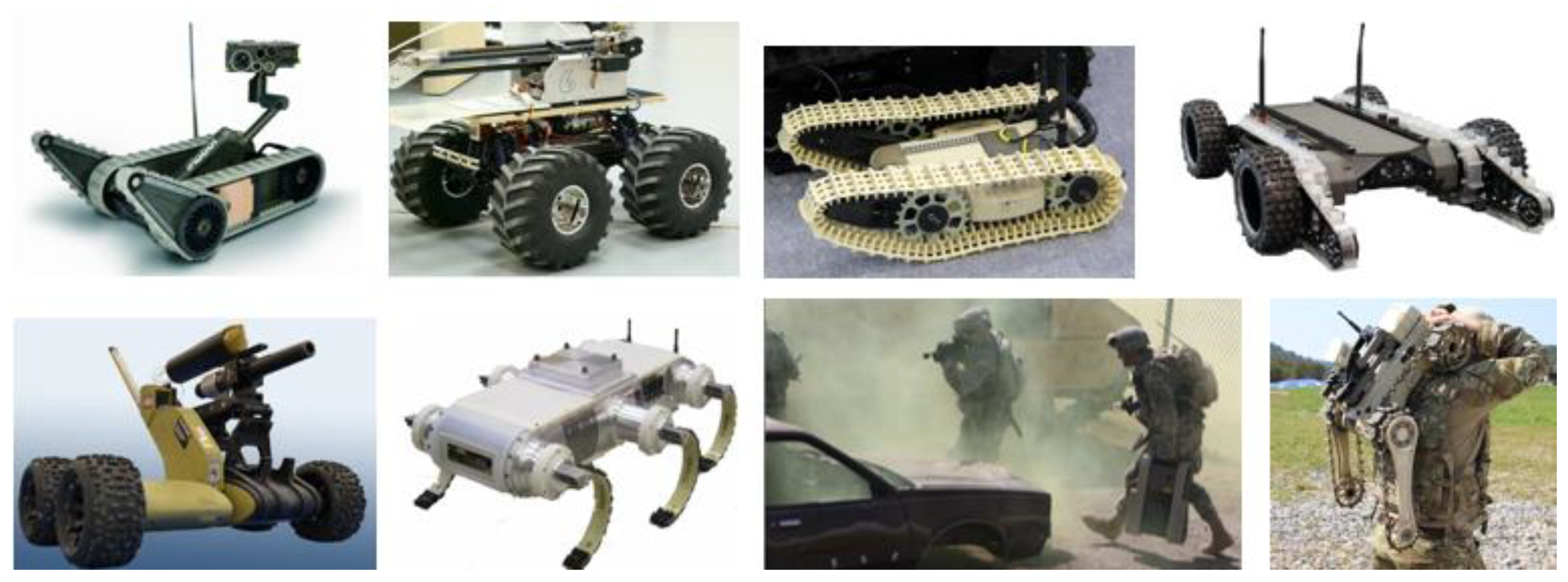
The miniaturization of all components of robotic systems has led to the emergence of a new class of mobile robots—compact and lightweight mobile mini-robots (MMR). MMRs are small-sized rapid response robotic vehicles that can be quickly transported and deployed by one person (i.e., an operator). Compact size and low weight allow this type of mobile robot to be classified as portable robotic systems, which fundamentally distinguishes them from larger mobile robots [3]. Some examples of the MMRs are shown in Figure 1.

MMRs are used in the field of security and military operations when solving the following tasks:

• Situational awareness (i.e., reconnaissance of the operational situation in hard-to-reach and/or dangerous places, e.g., inside premises, shelters, basements, caves, under vehicles, in vehicles interiors, etc.);
• Audio and video surveillance;
• Security and inspection of premises and restricted areas;
• Premises mapping;
• Examination and search for dangerous objects;
• Light cargo transportation (delivery).

MMRs are intended for use mainly in the urban environment (indoors and outdoors) providing round-the-clock and all-weather operation.

The main design challenge for these miniature robots is to ensure their locomotion in a nondeterministic environment in an urbanized area [4,5], which is characterized by obstacles that are comparable or exceed the robot’s own dimensions [6]. A key feature of MMRs is their low weight, which in most known designs ranges from 7 or 8 to 15 kg [3]. The distinctive advantages of MMR are also their low visibility and relatively high mobility. Typical travel speeds for MMRs are up to 2 or 3 m/s (7 to 11 km/h) with typical dimensions of the robot not more than 0.5 to 0.8 m (in length), and usual mover sizes (e.g., wheel diameter) not more than 0.10 to 0.15 m. If we compare these characteristics with larger robots with ordinary sizes of their movers of about 0.5 m, then this would correspond to their speeds of up to 15 m/s (more than 50 km/h) or speeds of up to 100 km/h for robots comparable in size to an average car.

The study of the theory and practice of designing wheeled and tracked vehicles, as well as mobile robots, shows that existing methods and approaches cannot be formally transferred to MMR small-sized transport systems [7], which have some features that distinguish them from larger machines (e.g., larger mobile robots, tracked and wheeled tractors, etc.). These features include:

• Small size of all components of drives and chassis, which leads to differences in the nature of interaction with the supporting surface;
• Functioning in an environment with macro obstacles (i.e., obstacles comparable to or larger than the robot itself);
• Need for more accurate accounting of internal losses in all components of a miniature transport system, which begin to play a significant role in relation to useful forces, especially taking into account relatively high speeds.

In the design practice of automotive and tractor vehicles, when carrying out traction prediction studies and choosing powertrain components, a widely used approach is to take into account internal losses in the transmission (gears, gearbox, final gear) in the form of constant efficiency [8,9,10,11,12,13]. Of course, the works on the design of electric vehicles and hybrid electric vehicles are much closer to the subject of this article. However, the same situation is observed in such works too [14,15,16,17,18,19].

This approach, in the general case, is justified for automotive and tractor vehicles, where the problem of accurately estimating internal losses in powertrain components is not so crucial during the design process. At the same time, this is not acceptable for the problem of modeling miniature transport systems of MMRs, where internal resistances may be comparable with useful forces in some load modes.

Consideration of the internal resistance in the tracks also plays a significant role in the design of tracked vehicles. Quite often, to simplify design calculations of the efficiency of tracks, they are also taken as constant values [13,20]. This is largely due to the lack of experimental data and the great complexity of analytical accounting for all components of the mechanical losses of a specific design of the tracked mover unit. In some studies [10,12], methods of experimental determination of the efficiency of tracks are given. In [10,11,12], empirical dependencies obtained on some specific transport vehicles are also given. However, these and similar dependencies are difficult to apply in practice, and even more, they are of little use for small-sized transport systems of mobile robots considered in this article.

The coefficients of rolling resistance and adhesion, which are given in the literature on common wheeled and tracked vehicles [9,10,11,21], are also inapplicable for MMRs.

Most of the research on small-sized mobile robots (e.g., [22,23,24,25,26,27,28,29]) is focused on the problem of a robot following a path and do not touch on the issues of modeling the robots’ drivetrains, determining the mechanical loads on their components and energy consumption, and assessing the computational accuracy of these items. Other studies [30,31,32] present and describe certain designs of the small-sized off-road mobile robots, simulate obstacles negotiation, but without considering analysis of drivetrain loads.

In this situation, following directly the recommendations and approaches that can be found in the literature on the theory of automotive and tractor vehicles, as well as on mobile robots of various types, when transferred to the field of development and modeling of miniature transport systems of MMRs can lead to great errors and incorrect results. This fact, which was confirmed during preliminary experimental tests, determined the relevance of this study.

This work is aimed at developing a methodology for a computer model composition of the MMR transport system based on identifying the particularities (factors) of the mathematical description of small-sized transport systems that are critical in terms of the calculated results. The article proposes a sequence for the development of a reliable computer model that allows for obtaining accurate simulation data. The resulting model is verified by experimental research. In conclusion, a comparative analysis of the model based on the proposed methodology is carried out with models built without taking into account the factors listed in the article, i.e., based on “traditional” approaches that follow from the analysis of the literature on the design of large transport vehicles and mobile robots. An evaluation of the convergences of the experimental data and the simulated data obtained using the proposed model and the simplified models showed that the proposed approaches to the computer models development can increase the accuracy of simulations (as a difference in the calculated errors) by 10 to 25% at maximum loading modes, and up to 30 to 70% at low and medium loading modes.

The main contribution of this article is to increase the efficiency of design work on the development of highly mobile small-sized ground robots, due to increasing the accuracy of dynamic calculations of their locomotion subsystems when following the proposed methodology. The results of the study can be useful for building computer models of small-sized mobile robots to study their operating modes, both at the stage of robot development and at the stage of assessing the characteristics and critical operating modes of an existing robot.

This article is based on and significantly expands and supplements a conference paper [33]. Note that the methodology for the design of the MMR transport system development and its structural composition is beyond the scope of this article. Therefore, the article provides only a brief description of the considered design “as is”. Also, note that the proposed methodology is used to build a complete computer model of the MMR transport system, including a subsystem for chassis geometric variation. This model allows for simulating both MMR locomotion on a flat non-deformable surface and overcoming obstacles (e.g., a single step, a stair). However, this article only considers the study of locomotion on a flat solid surface.

2. Fundamentals

2.1. Definition of the Term “Transport System”

The item of research of this article is the transport system of the MMR as an electromechanical device only. Therefore, the robot control system has been excluded from the concept of the term “transport system” in order to simplify its analysis. In this case, the control actions during the analysis are transmitted directly to the executive motors.

The term “transport system” in this study is understood as a set of elements directly involved in the process of sequential conversion of the energy of the on-board power source into mechanical energy of motion [34]. This energy transformation consists of three stages: distribution, conversion, and consumption.

A distributor is a set of devices that provide separation of the energy stream. Converters (actuators of the transport system) are divided into converters of electrical energy (i.e., executive motors) and converters of mechanical energy (i.e., mechanical transmission components). The undercarriage (running gear) acts as a consumer, which is considered in interaction with the support surface and thus forms the system known as the “terrain-vehicle system” [35]. The undercarriage is designed to ensure the movement of the mobile robot, to support its body, to reduce shocks, and to dampen vibrations. Thus, in the general case, the undercarriage comprises movers and a suspension system.

This approach to the definition of the research item allows us to consider the proposed computer model of the transport system as a component of the full model of a mobile robot, focusing on the development of the reliable model of this electromechanical component.

2.2. Description of the MMR Transport System

The transport system design decisions greatly affect both the final entire robot appearance and its functionality (including adaptability to locomotion conditions, energy consumption, etc.). The validity of these decisions plays a key role in the design of a mobile robot. This is especially crucial for robots of mini- and micro-sizes since their transport systems are subject to increased requirements for passability due to their small dimensions [3,36]. As mentioned above, these MMRs must be able to navigate the terrain with obstacles comparable to or larger than the robot itself.

In this study, the task was to develop a transport system for MMR with a length of no more than 400 mm and a height of no more than 100 mm, which would nevertheless allow the MMR to:

• Have a mass of no more than 15 kg;
• Move along stairs inside buildings;
• Overcome single obstacles in the form of steps of 300 mm high;
• Move at a speed of at least 1 m/s;
• Have a battery life of at least 3 to 4 h.

The result of the proposed solution for the MMR chassis in the form of a kinematic layout is shown in Figure 2. This design layout was obtained in accordance with the methodology of [37] and represents chassis in two configuration options: tracked (indicated in the figure with formula 6T2A) and wheeled (indicated as 4W2T). Hereinafter, the designations of the chassis formulas are given in accordance with [38].

The tracked configuration 6T2A is a six-track chassis (6T) with two tractive drives and two active (2A) degrees of freedom (DoF) of the chassis geometry variation (CGV) mechanisms with drives for tilting of the front and rear pairs of the levers (also known as flippers) with additional tracks. The following designations are shown in Figure 2: P_t1 and P_t2 are the traction forces on the left and right tracks, M_p1 and M_p2 are the torques on the front and rear CGV drives.

Thus, we can say that the transport system of the MMR under consideration comprises two subsystems: the locomotion subsystem (which this article is mainly devoted to) and the chassis geometric reconfiguration subsystem (i.e., CGV).

The wheeled configuration 4W2T is obtained by detaching the flippers from the basic 6T2A chassis and replacing them with wheels. This results in an all-wheel-drive (4W) chassis with front wheel drives, in which torque is transmitted to the rear wheels by means of two main tracks (2T).

As Figure 3 shows, the MMR transport system structure is a sequential chain of links “power source–motors–gearboxes–undercarriage (chassis) in interaction with the supporting surface”. A specialty of this structure diagram is that its electromechanical system branches through a power distribution device (PDD) into two relatively independent drive subsystems: a subsystem of i-tractive drives and a subsystem of j-drives of CGV.

As can be seen from Figure 3, the subsystem for controlling the executive drives of the transport system is conditionally separated from it, since the transport system, as mentioned earlier, is considered only as an electromechanical component of the MMR. Thus, the control actions on the transport system drives (the levels of supply voltages on the motors) are considered as known and are taken into account as the initial analysis data [34]. In this case, the drive motors are considered to be connected directly to the power source PS through the simplest switching device (PDD in Figure 3) that connects the necessary motor to the power source PS at the right time.

2.3. Structural Composition of the MMR Transport System

Each of the i-drives and j-drives from the drive subsystem (I) in Figure 3 is represented by an electric motor and a set of mechanical transmission devices, the composition of which is determined, among other things, from the design and layout solutions of the entire MMR. It is important to note that, considering the small size of the mini-robot, the layout of all its parts as a whole can significantly affect the composition of the transport system components and should be carried out initially at the first stages of its design development in order to check the principal feasibility of the scheme solutions developed in Section 2.2, taking into account previously defined geometric parameters [37].

Figure A1 of Appendix A shows one of the possible variants of the structural–kinematic scheme of the transport system, and Figure A2 of Appendix A shows the layout diagram of the MMR corresponding to this design variant.

3. Materials and Methods

This section is structured as follows: (1) A dynamic analysis scheme is presented and a brief mathematical description of the components of the MMR transport system is given, indicating the identified features that are essential for small-sized electromechanical components of transport systems for these mobile robots. (2) The methods and results of experimental identification of the parameters of the MMR transport system components are described. (3) The proposed method for constructing a complete computer model of the MMR transport system is described and a brief description of its characteristics given. (4) A description of the methods for conducting simulation and experimental studies of the MMR transport system moving on an inclined surface is given.

3.1. Dynamic Analysis Scheme of the MMR Transport System

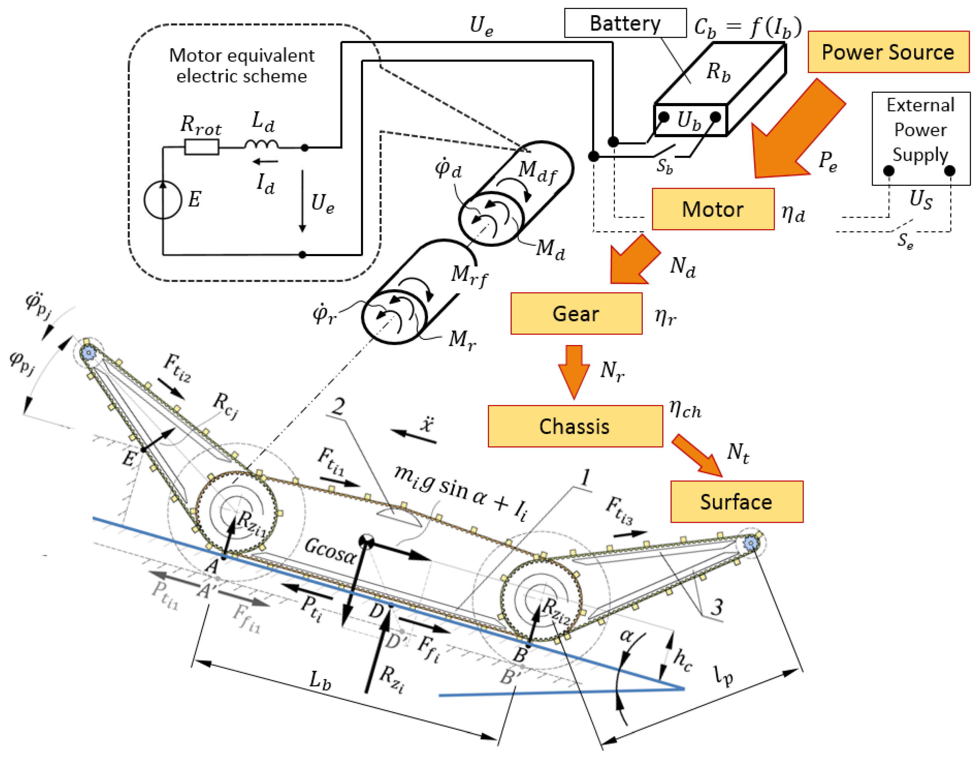
Figure 4 shows the dynamic analysis diagram of the transport system during the MMR rectilinear motion along a surface with a slope angle α. Only the drive branch of the left side is shown for simplicity.

Since this article describes the locomotion subsystem (i.e., the subsystem of tractive drives), only that aspect is discussed in more detail below.

Figure 4 illustrates the process of sequential conversion of energy in the MMR transport system from the block designated as “Power supply” to the block “Chassis” in interaction with the “Surface”. The following designations are adopted here: $P_e$ is the power delivered by the power source; $N_d$ is the motor output mechanical power; $N_r$ is the gear output power; $N_t$ is the power transmitted from the movers (i.e., tracks, wheels) to the surface; ${\eta }_d$ is the motor efficiency; ${\eta }_r$ is the gear efficiency; and ${\eta }_{ch}$ is the chassis efficiency.

Figure 4 also gives an idea of the design implementation of the MMR chassis. In the version presented, the design of the running gear is simplified as much as possible to reduce weight. The MMR track mover is a toothed belt transmission based on polyurethane reinforced belts with grousers welded on the outer surface. There are two toothed pulleys, along the edges of the track contour, which play the role of support rollers of the chassis, one of which (front) is a drive. Rigid supporting and guiding elements are used that are indicated in Figure 4 as follows: 1—lower supporting guide of the main track; 2—upper guide of the main track (damper–tensioner); and 3—supporting guides of additional tracks on the flippers.

The interaction of the movers with the surface is characterized by the relation of traction forces $P_t$, cohesive forces $F_{\phi }$, motion resistance forces $F_f$, as well as gravity $G$, and normal reactions $R_z$ acting from the supporting surface.

The differential equation of steady-state motion of the robot in the direction of the x-axis, taking into account the assumption that the loads acting on each side are identical, has the form [34]:

$$\ddot{x}{m}_i{\delta }_i=P_{ti}-F_{fi}-m_{i}g\sin \alpha ,$$

(1)

where x is the coordinate of the center of mass of the robot along the axis of motion; $m_i$ is the conventional part of the MMR mass interacting with the i-th tractive drive; ${\delta }_i$ is the mass factor (i.e., the coefficient of rotating masses); $P_{ti}$ is the traction force developed by the movers of the i-th tractive drive; $F_{fi}$ is the motion resistance force of i-th mass; g is gravitational acceleration; α is surface slope angle (x-axis coincides with the direction of the largest elevation angle). I_i in Figure 4 is the inertial force acting on the i-th mass.

The mass factor ${\delta }_i$ in the absence of longitudinal sliding of the movers is found as [39]:

$${\delta }_i=\frac{J_{eq i}^{\prime }}{m_i{r}_k^2},$$

(2)

where $J_{eq i}^{\prime }$ is the equivalent moment of inertia, defined as:

$$J_{eq i}^{\prime }=m_i{r}_k^2+J_{di}\cdot i_{ri}^2{\eta }_{ri}+J_{ki}$$

(3)

where $r_k$ is the radius of the wheels (pulleys); $J_{di}$ is the rotor inertia of the motor; $i_{ri}$ is the total gear ratio; ${\eta }_{ri}$ is the total gear efficiency; $J_{ki}$ is the inertia of the drive wheels (pulleys) and their associated rotating parts.

Traction force is:

$$P_{ti}=\frac{M_{di}\cdot i_{ri}{\eta }_{ri}}{r_k}-F_{ti},$$

(4)

where $M_{di}$ is the motor torque and $F_{ti}$ is the total internal resistance force in the tracks of the i-th side.

Motion resistance force is

$$F_{fi} =f{m}_{i}g\cos \alpha ,$$

(5)

where $f$ is the rolling resistance coefficient.

The possibility of the propulsion force realization is determined by the adhesion condition [10,11,12,40], compiled for the machine as a whole in the form:

$${{\displaystyle \sum }}^{ }{P}_{ti}\le \phi Mg\cos \alpha ,$$

(6)

or individually for each board:

$$P_{ti}\le \phi R_{zi},$$

(7)

where $\phi$ is the coefficient of the mover to the surface adhesion; $M$ is the robot total mass; $R_{zi}$ is the normal force on the i-th track (wheel).

3.2. Features of the Mathematical Description of the MMR Transport System

A series of preliminary experimental tests of the components of the MMR transport system showed that for these MMRs it is necessary to take into account, in addition to the force-loading mode, also the speed-loading mode. It was established that the internal resistance in all mechanical components of the transport system significantly depends on speed. Ignoring this leads to significant computation errors that are unacceptable from a practical point of view, which is explained and confirmed in Section 5 of this article.

A brief mathematical description of the components comprising the MMR transport system according to Figure 4 is introduced below. Experimental identification of the parameters included in the characteristics presented below was also carried out in this part of the study (see Section 3.3).

3.2.1. Power Source

Considered in the first place, the “Power source” block (PSB) is designed to simulate the operating mode of the on-board power supply. The output signal of this block is the on-board supply voltage $U_e$, which is then supplied to the drives of the transport system through the “Power Distribution” unit (not shown in Figure 4).

Depending on the selected mode, the output branch of the “Power source” block is connected either to the on-board battery with a voltage of $U_b$ (Source Mode 1) or to an external power supply with a fixed voltage $U_S$ (Source Mode 2). The second mode is necessary for the study of various speed-loading modes of the transport system obtained by variation the supply voltage $U_e$.

Thus, the setting of the operating modes of the PSB is described as follows:

$$U_e=\{\begin{array}{c}{U}_b, if Source Mode=1\\ U_S, if Source Mode=2.\end{array}$$

(8)

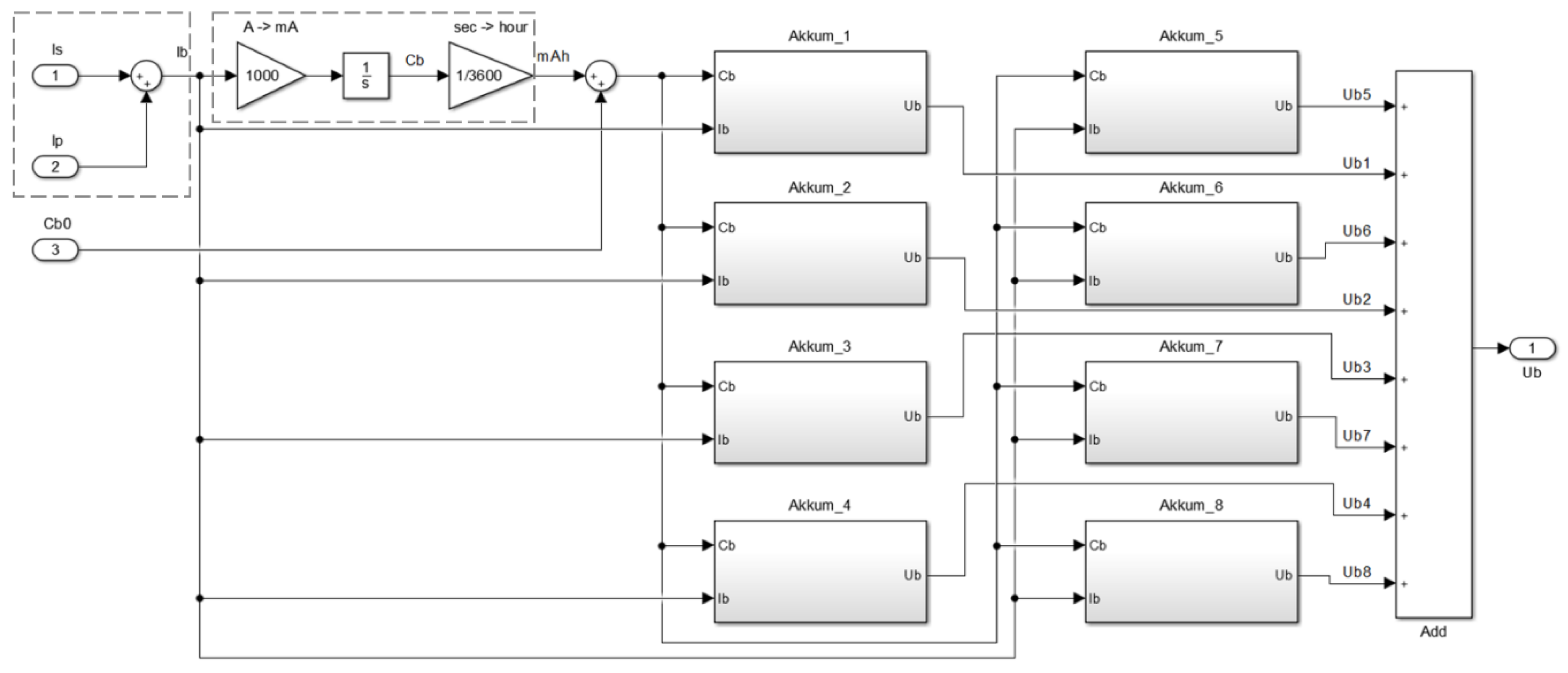
The “Battery” block simulates an on-board MMR battery, consisting of eight Li–Po accumulator elements (i.e., battery cells) connected in series and named as “Akkum_1”... “Akkum_8” so that the output voltage of the entire battery is:

$$U_b={\sum }^{ }{U}_{bi}$$

(9)

where $U_b$ is the battery cell voltage and i = 1...8 is the battery cell number.

The values of the battery total load current $I_b$ and the accumulated degree of discharge of the battery $C_b$ are determined as follows:

$$I_b=I_s+I_p,$$

(10)

$$C_b=\int I_b dt,$$

(11)

where $I_s$ is the total current of all the motors (i.e., the sum of the motor currents $I_d$) of the transport system and $I_p$ is the total current of all other MMR consumers not related to the transport system.

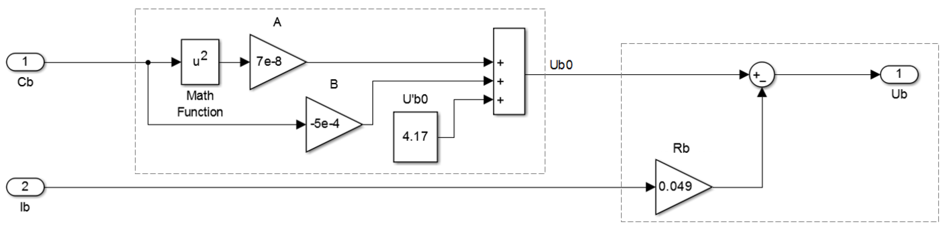
The calculation of the output voltage $U_{bi}$ on the battery cells is accounted for by the following expressions:

$$U_{bi}=U_{b0 i}-I_b{R}_{bi},$$

(12)

$$U_{b0 i}=A\cdot C_b^2+B\cdot C_b+U_{bo i}^{\prime },$$

(13)

where $U_{b0 i}$ is a battery cell no-load voltage; $R_{bi}$ is the self-electric resistance of a battery cell; A and B are experimental statistical coefficients (defined in Section 3.3.1); $U_{bo i}^{\prime }$ is an initial no-load battery cell voltage.

Therefore, when calculating the on-board battery voltage $U_b$, the voltage drop in the battery is taken into account under the action of the total current load from all consumers of the MMR and the accumulated discharge capacity.

3.2.2. Motors

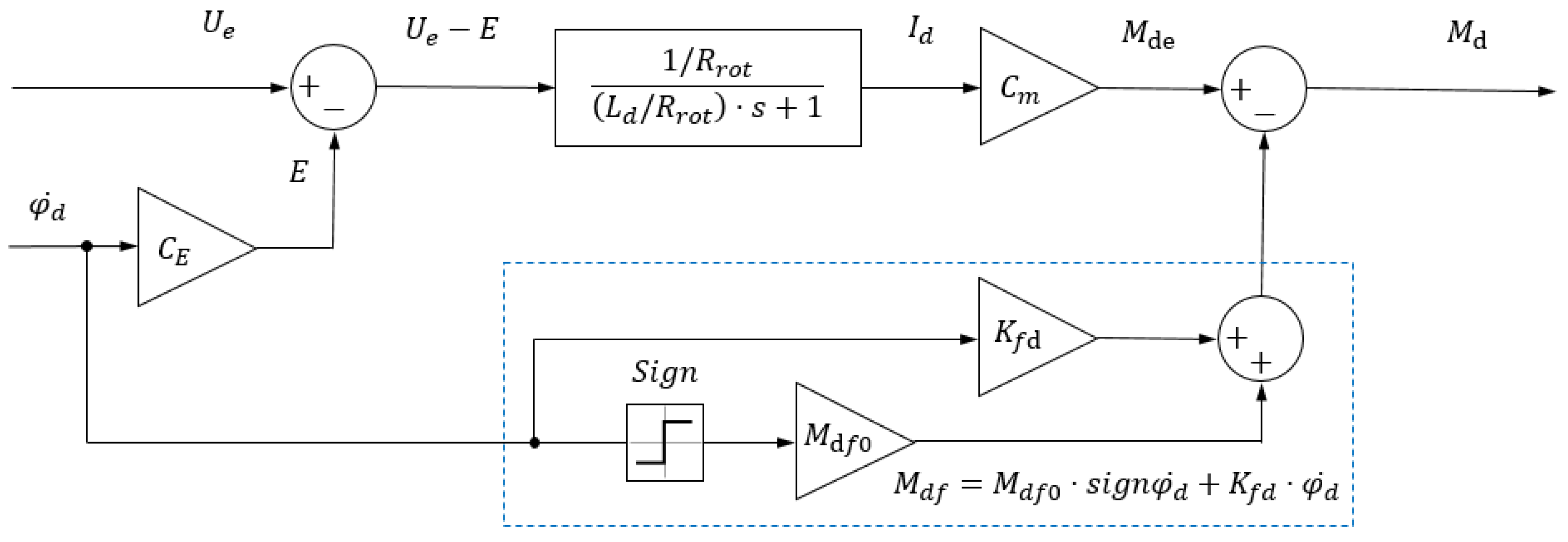
The “Motor” blocks are models of electric motors of the locomotion subsystem (i.e., the subsystem of tractive drives). Their construction is based on well-known mathematical models that describe the dynamics of DC motors [41,42,43]. However, a distinctive feature of the suggested model is the introduction of the torque of internal resistance forces of the motor $M_{df}$ in a form that includes a dependence on the rotational speed of the motor shaft and has the form

$$M_{df}=M_{df0}\cdot sign\left({\dot{\phi }}_d\right)+K_{fd}\cdot {\dot{\phi }}_d,$$

(14)

where $M_{df0}$ is the motor dry friction torque (i.e., Coulomb friction); ${\phi }_d$ is the rotation angle of the motor shaft; $K_{fd}$ is the coefficient of viscous friction.

The motor model, in addition to Equation (14), is represented as follows:

$$U_e=E+I_d{R}_{rot}+L_{d }\frac{d{I}_d}{dt},$$

(15)

$$E=C_E{\dot{\phi }}_d,$$

(16)

$$M_{de}=C_m{I}_d,$$

(17)

$$M_d =M_{de}-M_{df},$$

(18)

where $E$ is the back-electromotive force; $I_d$ is the motor current; $R_{rot}$ is the motor terminal resistance; $L_d$ is the motor terminal inductance; $C_E$ is the motor speed constant; $M_{de}$ is the motor electromagnetic torque; $C_m$ is the motor torque constant; $M_d$ is the motor mechanical torque.

The model presented does not take into account the inertia of rotating masses accelerated by electric motors, because the equivalent moments of inertia are taken into account in the model of the executive subsystem of the MMR transport system (Section 3.4.3).

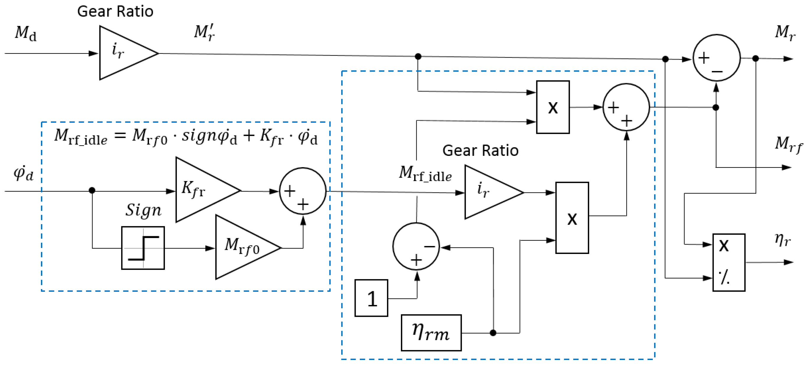
3.2.3. Gears

The “Gear” blocks simulate the reduction gear units of the transport system.

A distinctive feature of the model presented is that it takes into account the variability of the torque of internal losses and the gear efficiency, as well as the dependence of the internal friction in the gearbox on speed.

When calculating and modeling large vehicles and mobile robots, losses in mechanical transmissions are traditionally taken into account as constant values calculated for certain nominal values of the external load [8,9,10,11,12,13,14,15,16,17,18,19,34,42,44]. This is permissible when considering operating modes of reduction gears at loads equal to or greater than nominal. However, strictly speaking, when a mobile robot moves, the loads on the mechanical gears change within a much wider range, which requires a more accurate consideration of the characteristics of mechanical losses in reduction gears under partial load conditions.

It is known that the internal losses of the gearbox are composed of no-load losses and losses proportional to the external load, and can be described as [20,45]:

$${\eta }_r=\left(1-\frac{M_{rf\_idle}}{M_d}\right){\eta }_{rm}=\frac{M_r}{M_d i_r},$$

(19)

where ${\eta }_r$ is the gearbox efficiency; $M_{rf\_idle}$ is idle loss torque of the gearbox reduced to the input shaft; $M_d$ is the torque on the input shaft of the gearbox (output shaft of the motor); ${\eta }_{rm}$ is the efficiency taking into account losses proportional to an external load (maximum value); $M_r$ is the torque on the output shaft of the gearbox; $i_r$ is the gear ratio.

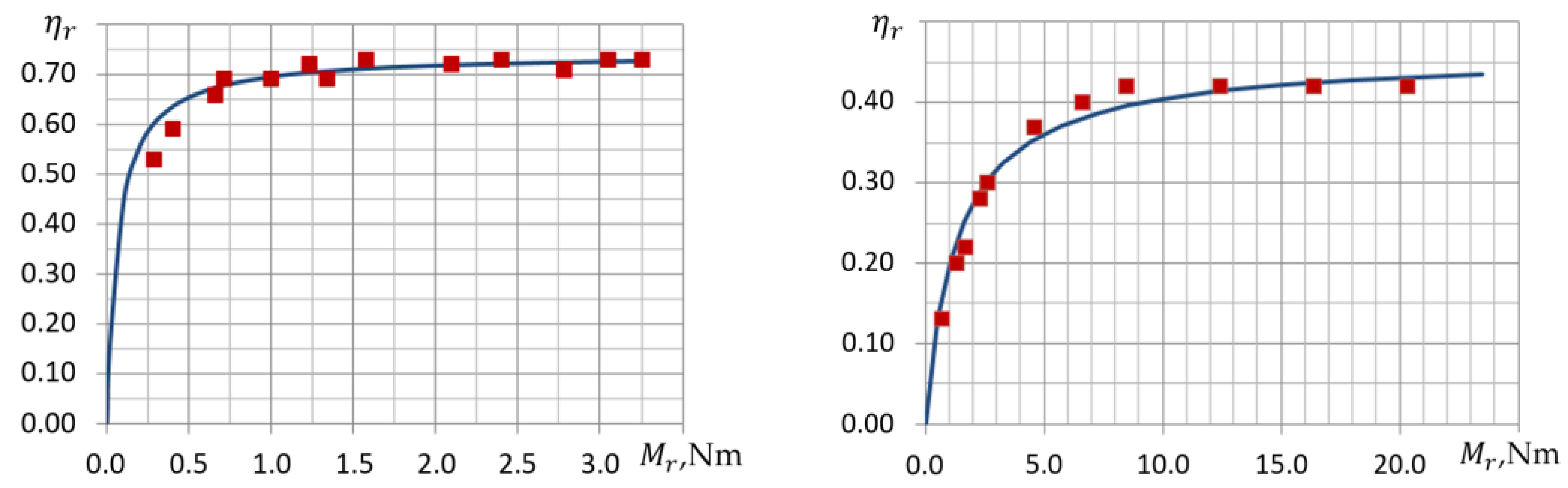
The efficiency characteristics of the gearboxes depending on the output torque $M_r$, constructed according to (19), have the form shown in Figure 5. The shape form of these dependencies is widely known from the theory of machine parts design [34], and their quantitative description is in good agreement with the results of experimental studies on gears used in the transport system under consideration.

Experimental studies of the elements of small-sized MMR transport systems have shown that the torque of the gear idle loss $M_{rf\_idle}$ has a significant effect on the total value of internal losses and is described by the dependence

$$M_{rf\_idle}=M_{rf0}\cdot sign {\dot{\phi }}_d+K_{fr}\cdot {\dot{\phi }}_d,$$

(20)

where $M_{rf0}$ is the gear Coulomb friction torque measured on the gear’s input shaft; ${\phi }_d$ is the rotation angle of the gear input shaft; $K_{fr}$ is the coefficient of viscous friction.

The total torque of internal resistance in the reduction gear expressed at the output shaft is defined as

$$M_{rf}=M_d i_r\left(1-{\eta }_r\right)$$

(21)

Then from (21), taking into account (19), we have:

$$M_{rf}=M_d{i}_r\left(1-{\eta }_{rm}\right)+M_{rf\_idle} i_r {\eta }_{rm}.$$

(22)

Equation (22) represents losses in the gearbox as the sum of losses proportional to the load torque (first term) and idle losses (second term).

The torque on the output of the gearbox unit is as follows:

$$M_r=M_d{i}_r-M_{rf}.$$

(23)

3.2.4. Chassis

A significant part of the internal losses of the transport system occurs in the chassis elements. The value and reasons for the occurrence of losses in the chassis unit are largely determined by its constructive design, the diagram of which is shown in Figure 4.

In general, losses in the chassis of the MMR are associated with the following factors:

• Coulomb friction of the tracks on the guiding elements of the body (or rolling friction when using track rollers);
• Impact interaction and friction of the engaged elements of the “track – drive wheel” subsystem;
• Resistance to track bending;
• The impact interaction of the support elements of the track when they come into contact with the surface.

It should be kept in mind that the dependences characterizing the factors noted are periodic in nature, caused by both the periodic structure of the track itself and its oscillations. Moreover, the dynamics of these oscillatory processes are associated with the speed of the track. An increase in speed causes an increase in the frequency of vibrational disturbances, which, according to the theory of oscillations of nonlinear mechanical systems [46], leads to the appearance of the pseudo transformation of dry friction forces into viscous friction forces, i.e., the dependence of friction forces on speed. In this case, the generalized torque of internal resistance forces in the track is represented as

$$M_t=M_{t0}\cdot sign {\dot{\phi }}_k+K_{ft}\cdot {\dot{\phi }}_k,$$

(24)

where $M_{t0}$ is the initial (static) torque of the internal friction forces of the track; ${\phi }_k$ is the rotation angle of the drive wheel (pulley); $K_{ft}$ is the coefficient of pseudo viscous friction.

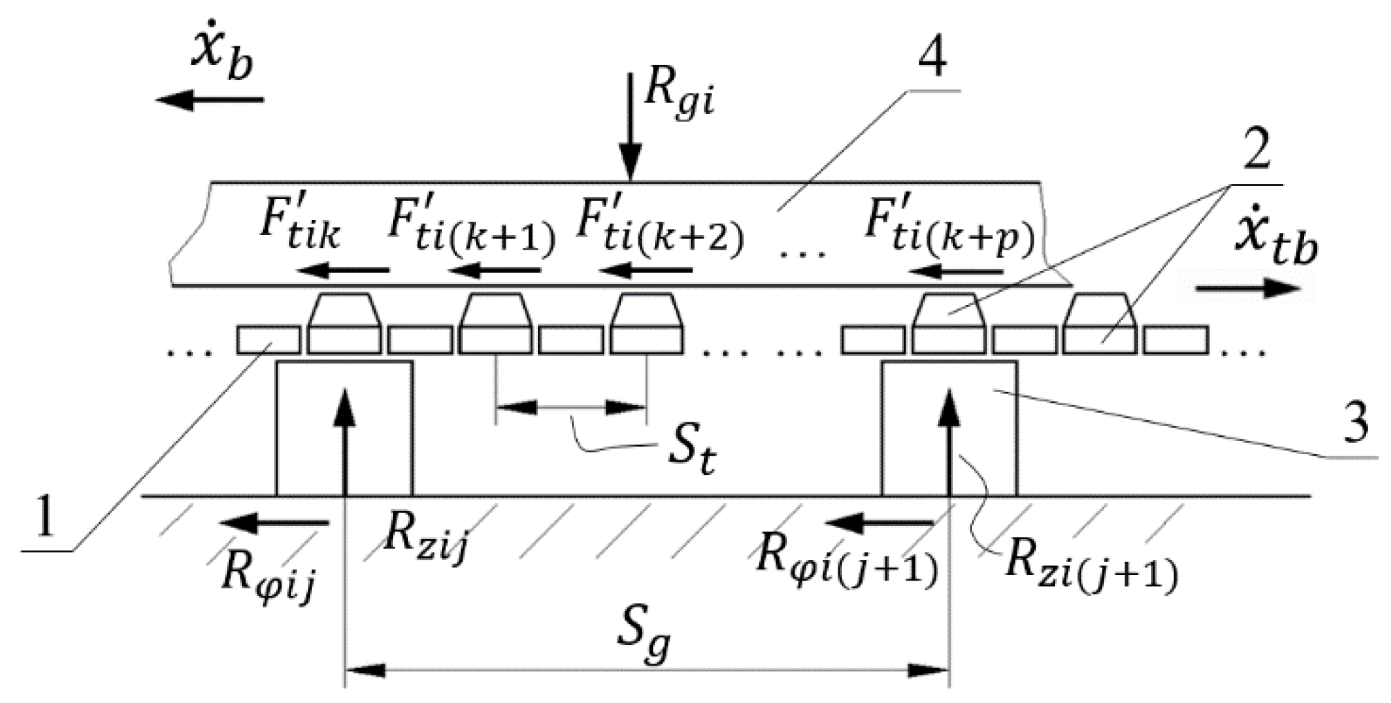
The diagram for constructing a design model for the interaction of a chassis track with a solid non-deformable base and robot body elements, drawn in accordance with the design of the tracked mover described in Section 3.1, is shown in Figure 6.

To simulate a chassis track as a flexible body, it is represented in the form of a sequential chain of typical links of three types: a rectangular support element 1, a working tooth 2 of a trapezoidal shape mounted on a support element of a track, and a grouser 3 of the rectangular form, rigidly fixed to element 2 on the outside of the track. The working teeth of the track (element 2) follow with a pitch $S_t$ equal to 5 mm, the grousers follow with a pitch $S_g$ of 35 mm. Links 1 and 2 are connected by conventional joints with one DoF.

During its operation, the track is in contact with the following elements:

• Driving and driven pulleys through the engagement of the teeth 2 of the track with the teeth of the pulleys (not shown in Figure 6);
• A support base (i.e., with a flat surface in the example of Figure 6) through the grousers 3;
• A supporting surface through elements 1, 2, and 3 when driving over obstacles on an uneven surface (see point E in Figure 4);
• The MMR body (through the lower and upper guides, shown respectively under position 4 in Figure 6 and position 2 in Figure 4).

Figure 6 shows a diagram of the forces acting on the support section of the track. Indices designate: $i$ is the serial number of the side of the chassis ($i$ = 1 ... 2); $j$ is the serial number of the grouser ($j$ = 1 ... 24 for the main track, and $j$ = 1 ... 16 for additional tracks of the flippers); $k$ is the serial number of the working tooth of the track ($k$ = 1 ... 168 for the main track, and $k$ = 1 ... 112 for additional tracks).

In accordance with the diagram presented, the following forces act on the track:

• Weight force $R_{gi}$ (part of the robot’s weight acting on its i-th side through guide 4);
• Friction forces $F_{t ik}^{\prime }$ of the k-th working tooth on the guide 4;
• Normal reactions of the supporting surface $R_{z ij}$;
• Adhesion forces $R_{\phi ij}$ of j-th grousers with the surface.

The track itself, in addition to the forces indicated in Figure 6, is under the action of the traction force $P_{ti}$, the centrifugal force $P_{cti}$, and the pre-tensioning force of the track P_0i [47]. In addition, when the traction force $P_{ti}$ exceeds the total adhesion force $R_{\phi ij}$, the track slips relative to the surface.

In this case, the contact interaction of the main track with the surface is characterized by the friction of the grousers against it with a total force

$$F_{t{g}_i}={\displaystyle \sum }_{j=1}^p{F}_{t{g}_{ij}}={\mu }_g{\displaystyle \sum }_{j=1}^p{R}_{z_{ij}}, p=1\dots 24,$$

(25)

where ${\mu }_g$ is the grousers–surface friction coefficient and $p$ is the number of grousers of the track.

Similar to the last expression, the total friction force of the track on the body guides is

$$F_{t_i}^{\prime }={\displaystyle \sum }_{k=1}^s{F}_{t_{ik}}^{\prime }={\mu }_t{\displaystyle \sum }_{k=1}^s{R}_{g_{ik}}, s=1\dots 168,$$

(26)

where ${\mu }_t$ is the track–body friction coefficient and $s$ is the number of working teeth of the track.

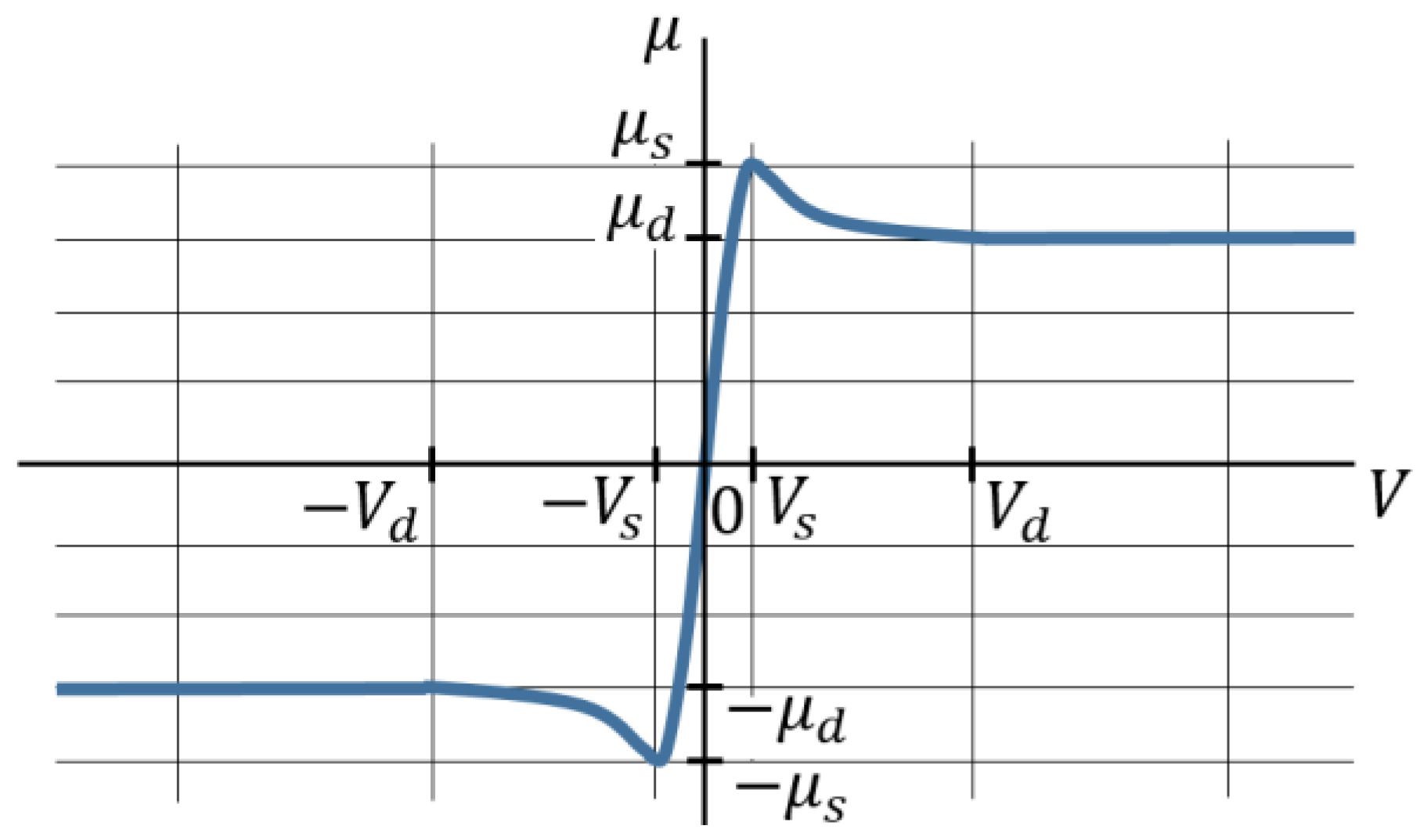
Equations (25) and (26) correspond to the description of the Coulomb friction model [25]. The current values of the friction coefficients ${\mu }_t$ and ${\mu }_g$ are determined by the instantaneous mode of operation of the friction pair, which is calculated in accordance with the friction model shown in Figure 7 [48,49].

Under this model, the interaction of two rubbing bodies is determined by the relative speed of motion V and is described by three modes:

• Static friction, acting at speeds from zero to the maximum speed of the static friction mode $V_s$, the friction coefficient increases from zero to the static friction coefficient ${\mu }_s$;
• Transitional mode between static and dynamic friction at the speed range from $V_s$ to $V_d$ with a decrease of the friction coefficient from ${\mu }_s$ to ${\mu }_d$;
• Dynamic friction mode at speeds greater than $V_d$ with a dynamic friction coefficient ${\mu }_d$.

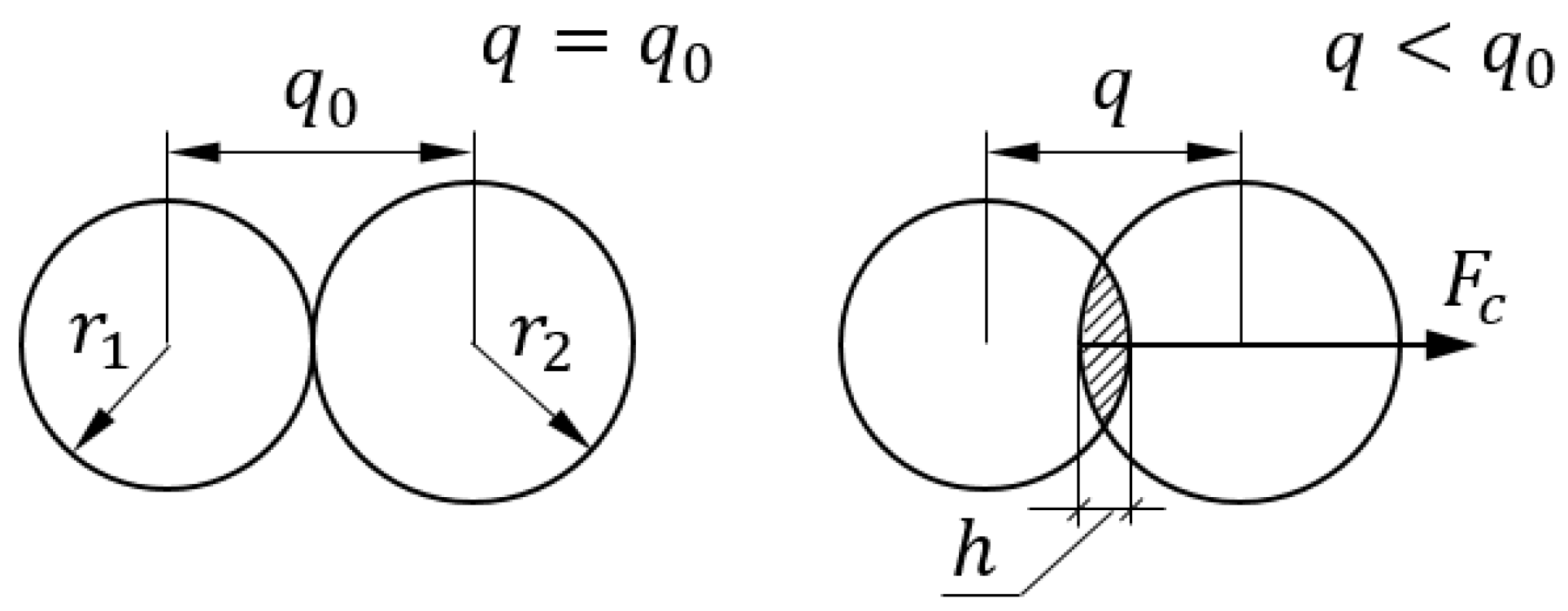
The description of contact interactions is carried out following the model shown in Figure 8.

Under this model, the contact force $F_c$ is determined as a function of the value h of mutual penetration of two bodies by the formula [48]:

$$F_c=\{\begin{array}{cc} 0,\hfill & \hfill if q\ge q_0,\\ c{h}^e -b_{max}\dot{q}\cdot step\left(q,q_0,d\right),\hfill & \hfill if q<q_0,\end{array}$$

(27)

where $c$ is the stiffness coefficient; $e$ is an empirical coefficient; $b_{max}$ is the damping factor; $q$ is the distance between bodies; $\dot{q}$ is the body’s approach speed.

Wherein:

$$h=q_0-q,$$

(28)

$$q_0=r_1+r_2,$$

(29)

where $r_1$ and $r_2$ are radius vectors to surfaces of bodies 1 and 2 along the line of their interaction.

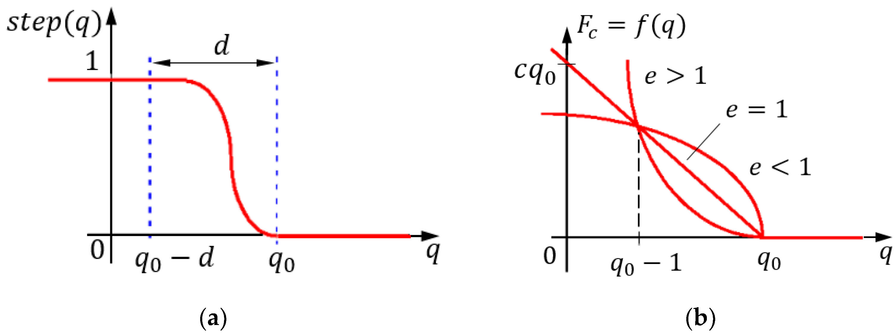
The step function in Formula (27) is a step function of the form shown in Figure 9a. It can be seen from the graph that the characteristic of this function is determined by the values of the parameters $q_0$ and $d$, where $d$ is the depth of interpenetration of the two bodies, at which the damping value changes from zero to the value $b_{max}$. The exponent $e$ in Formula (27) determines the nature of the change in $F_c$ in the static (i.e., steady-state) mode (at $\dot{q}$ = 0), as illustrated in Figure 9b, setting either the case of “hard” interaction (e > 1) or more “soft” interaction (e < 1).

3.3. Experimental Identification of the Models Parameters

This section describes the results of experimental studies carried out to determine the parameters of the MMR transport system component models described in Section 3.2. Experimental identification of the parameters of the on-board battery, motors, gearboxes, and chassis was performed.

3.3.1. On-Board Battery

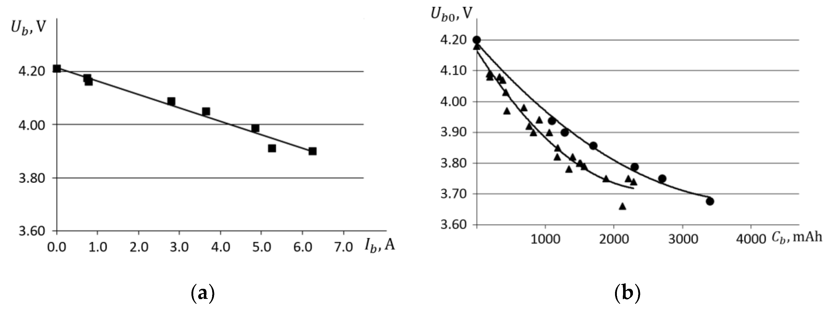
When the battery is discharged, the current value of $U_{b0}$ is in the range between some minimum and maximum values, which are determined based on the electrochemical system, the number and connection diagram of the primary battery cells, and the degree of battery discharge. Figure 10a shows the results of experiments to determine the load capacity of a fully charged ($U_{b0}$ = 4.2 V) lithium–polymer (Li–Po) battery cell. The character of the experimental dependence is in good agreement with the calculation by Equation (12). Therefore, the battery cell self-electric resistance $R_{bi}$ was determined as 0.049 Ohm. Figure 10b shows the results of an experimental study of the dependences of the no-load voltage $U_{b0}$ of Li–Po battery cells on the degree of their discharge, characterized by the value of the accumulated discharge capacity $C_b$. In Figure 10b, triangular markers indicate the results obtained on XP2200SL battery cells used in MMR; round markers indicate results for another battery cell model XP3700GT selected for comparison. As can be seen, these dependencies for both models of batteries are similar in shape and are approximated by a polynomial curve of the form determined by the Equation (13). The experimentally determined values of curve parameters and self-electric resistance of the battery cell used in the on-board battery of the transport system are shown in

Table 1. Battery cell experimental parameters.

Parameter	A	B	U’b0	Rbi
Units	V/(mah)2	V/(mah)	V	Ohm
Value	7 × 10−8	−5 × 10−4	4.17	0.049

.

3.3.2. Motor and Gears

In order to determine the parameters of the characteristic of the torque of internal resistance forces of the motor $M_{df}$ (Equation (14)), a number of tests were undertaken to measure the no–load currents $I_{df}$ at different speeds of rotation of the motor shaft (i.e., the motor supply voltage). Figure 11 shows graphs of the friction torques $M_{df}$ of several samples of the Maxon RE30 №310007 motor of the MMR transport system, obtained by recalculating the experimentally determined consumption currents $I_{df}$ in accordance with the expression

$$M_{df}=C_m{I}_{df},$$

(30)

where $C_m$ is the motor torque constant.

Similar tests were undertaken to identify the parameters of the characteristic of the torque of gearbox internal losses $M_{rf\_idle}$ (Equation (20)). For this, a series of tests carried out to study the no-load currents of the gear-motor assembly (Maxon RE30 motor + Maxon GP32C gear). Taking into account the fact that Equation (20) uses the moments reduced to the gear’s input shaft (i.e., corresponding to the output shaft of the motor), a similar method was applied for determining the torques through currents $I_d$ using Formula (30) adjusted for the values of previously determined motor friction torques $M_{df}$.

To determine the characteristics of the gearbox efficiency, the gear–motor assembly was tested on a dynamometer stand, which allows setting the values of the load moments using a load motor. The measurement of the output torque of the geared motor was carried out by a torque sensor. The results of experimental studies of the Maxon GP32C gearbox were presented earlier in Figure 5a.

The values of the experimentally determined parameters of the motor and gearbox models included in Equations (14), (20), and (22) are given in

Table 2. Motor and gear experimental parameters.

Parameter	Mdf0	Kfd	Mrf0	Kfr	ηrm
Units	mNm	mNm⋅s	mNm	mNm⋅s	–
Value	2.7	5.5 × 10−4	0.3	1.4 × 10−3	0.74

.

3.3.3. Chassis

The purpose of the experimental studies of the chassis was to determine the parameters of the characteristics of internal losses in the tracks (Equation (24)), and the parameters involved in the description of the interaction of the tracks with the surface of the robot locomotion and in the description of the interaction of the tracks with the elements of the robot body.

The determination of the parameters of the characteristics of internal friction in the components of the chassis was carried out by measuring the current consumption of the motors at the idle speed of the chassis. The results of identifying the parameters of the characteristics of the torques of internal losses in the tracked movers (Equation (24)) are given in

Table 3. Experimental parameters of the tracks.

Parameter	Mt01	Kft1	Mt03	Kft3
Units	mNm	mNm⋅s	mNm	mNm⋅s
Value	70	3	350	16

. The parameters related to one main track are designated as $M_{t01}$ and $K_{ft1}$. Parameters related to a total of three tracks on one chassis side are designated as $M_{t03}$ and $K_{ft3}$.

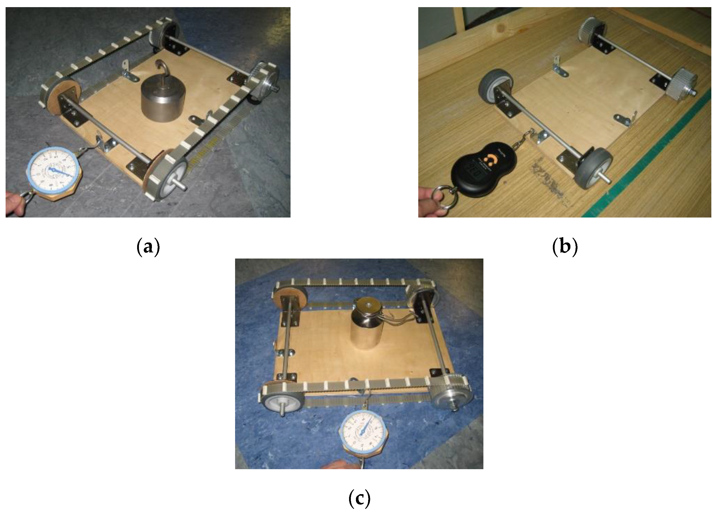
The small size and design features of the MMR running gear do not allow using the well-known values of the coefficients $f$ and $\phi$ [9,10,11,21] from the theory of ground transport vehicles for various typical road conditions. In this regard, it was required to conduct separate experimental studies. For this, a very simplified mock-up of the MMR chassis was used to exclude the influence on the measurements of internal friction in bearings, tracks, etc. Fragments of such studies, following the methods from [12], are shown in Figure 12.

The values of the experimentally determined coefficients of rolling resistance, as well as the coefficient of friction ${\mu }_t$ of the track along the guide of the robot body for the friction-pair polyurethane track–aluminum guide are given in

Table 4. Chassis experimental parameters.

Parameter	${\mathit{f}}_{\mathit{t}}$	${\mathit{f}}_{\mathit{w}}$	${\mathit{\mu }}_{\mathit{t}}$
Value	0.06	0.03	0.20

. The values of the experimentally determined coefficients of longitudinal adhesion ${\phi }_x$ and coefficients of lateral adhesion ${\phi }_y$ for various types of surfaces are given in

Table 5. Experimental values of adhesion coefficients on various surface types.

№	Surface Type	Tracked Chassis		Wheeled Chassis
		${\mathit{\phi }}_{\mathit{x}}$	${\mathit{\phi }}_{\mathit{y}}$	${\mathit{\phi }}_{\mathit{x}}$	${\mathit{\phi }}_{\mathit{y}}$
1	Linoleum	0.42	0.55	0.52	0.56
2	Smooth self-leveling concrete floor	0.45	0.55	0.60	0.62
3	Lacquered wood	0.32	0.38	0.38	0.43
4	Asphalt	0.68	0.70	0.60	0.62
5	Concrete	0.76	0.78	0.72	0.75

.

3.4. Computer Model Composition

3.4.1. Basic Conditions

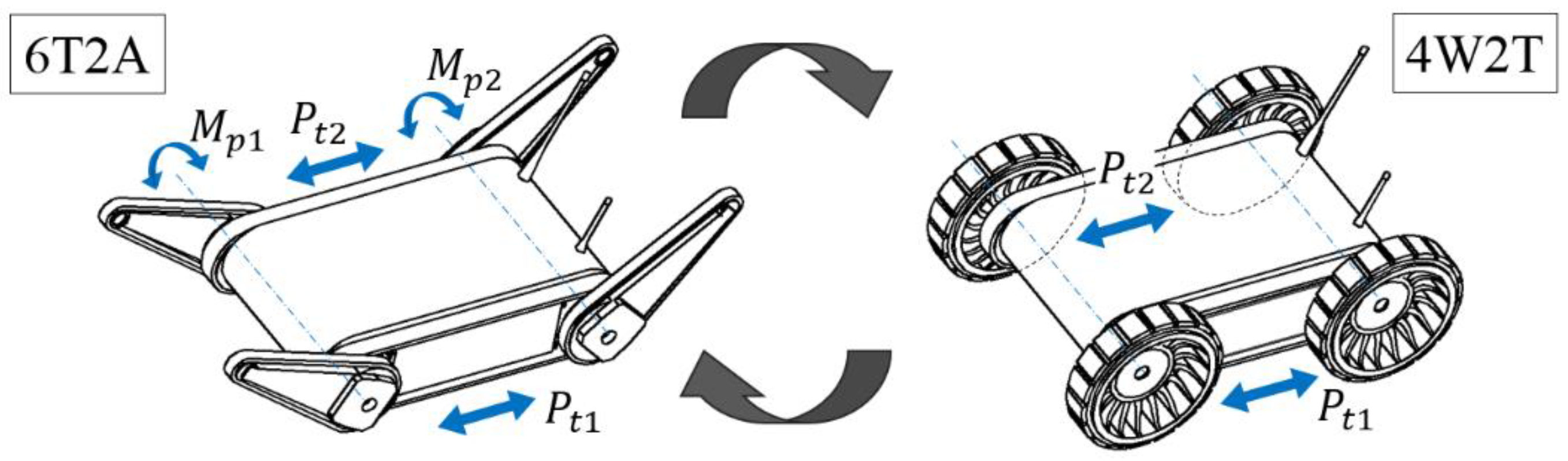
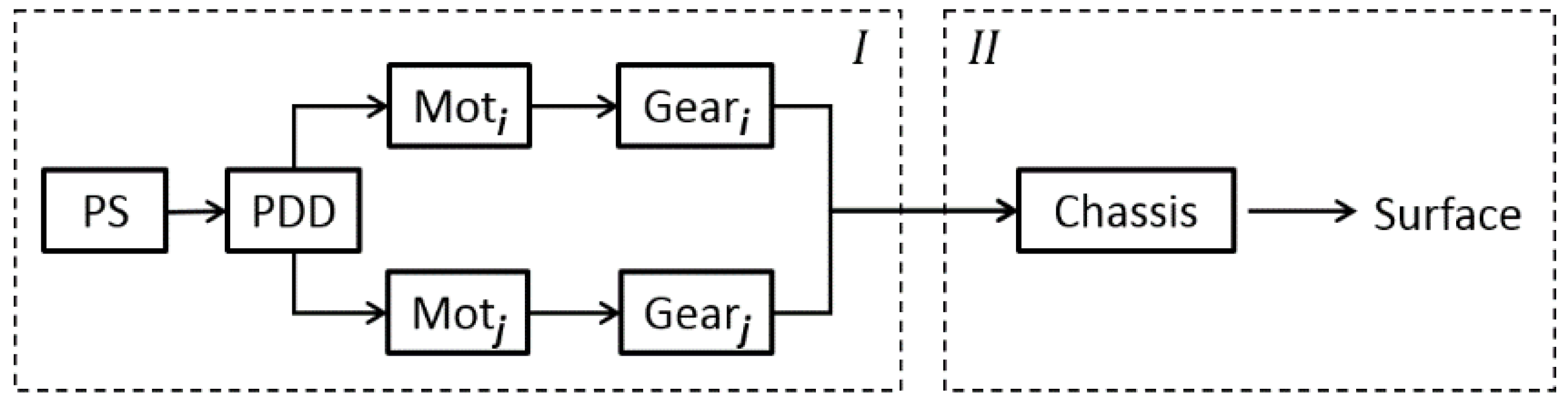
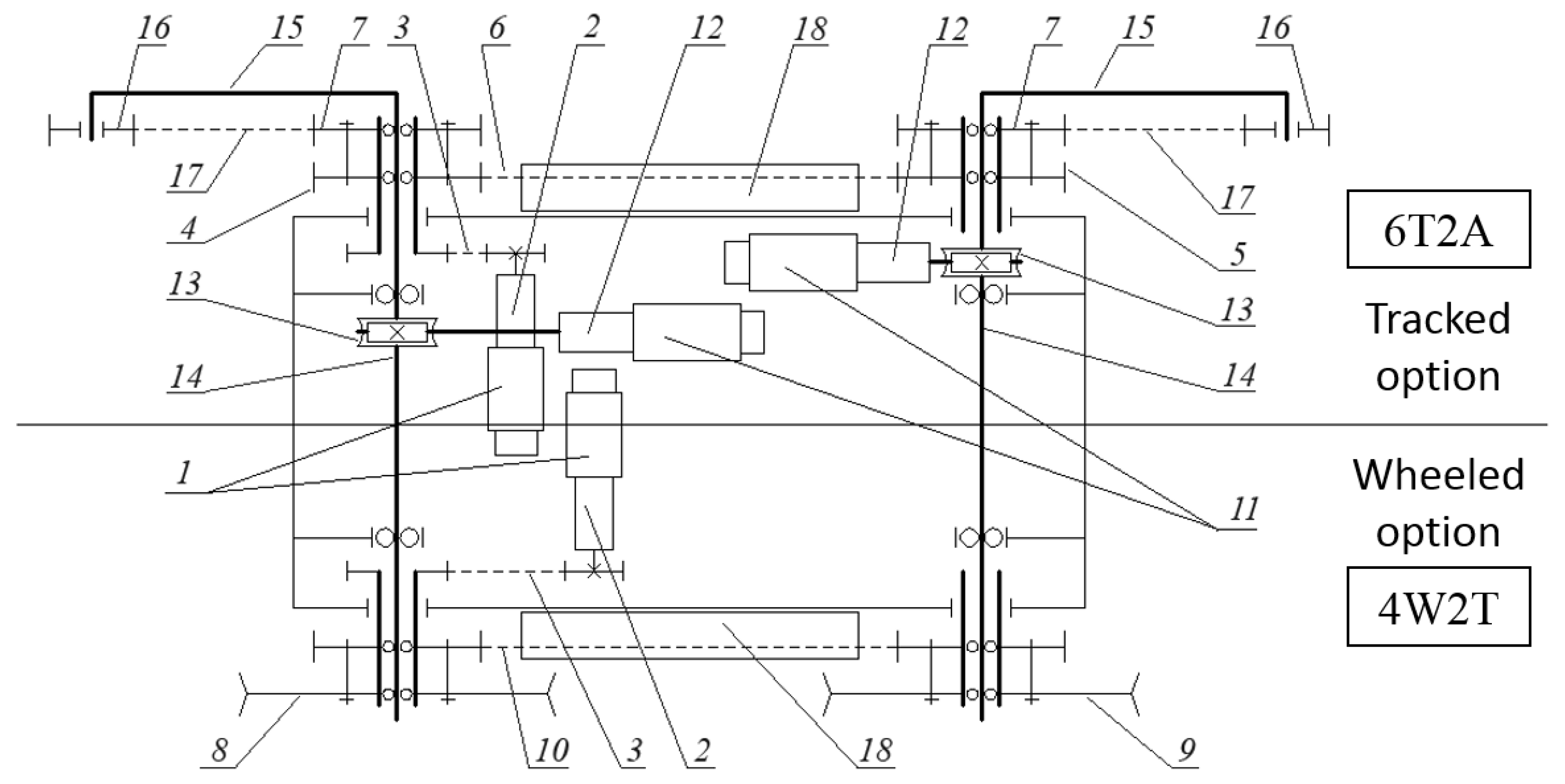
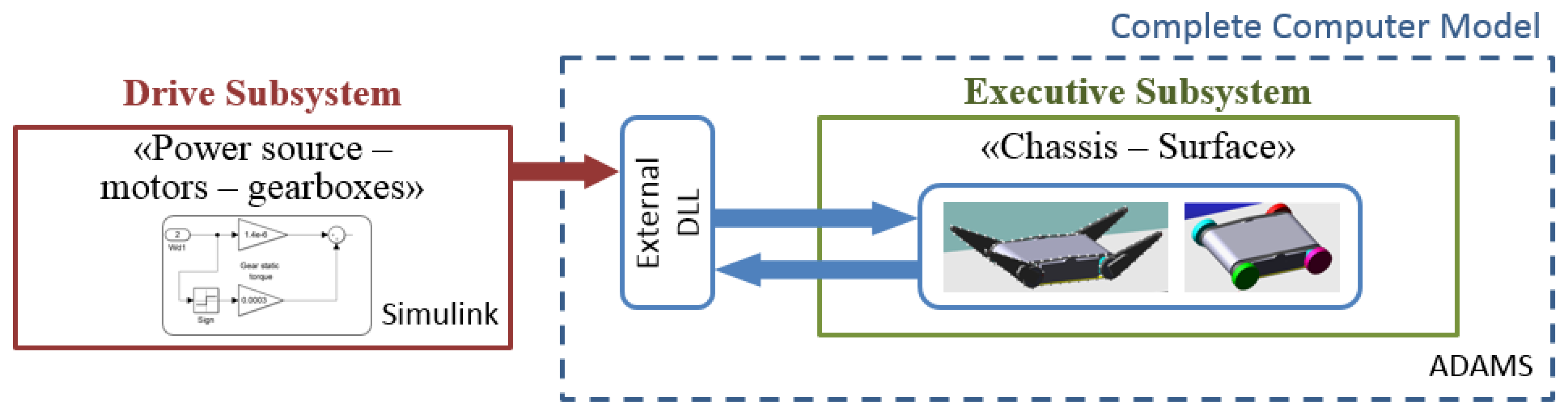
To conduct virtual studies of the transport system at various force and speed-loading modes, a computer (i.e., simulating) model of the transport system in both tracked and wheeled configurations was developed in accordance with the diagrams in Figure 3 and Figure 4. A feature of the model created is its division into two parts interacting with each other, schematically indicated in Figure 3 as the drive subsystem (I) and the executive subsystem (II).

The structure of the computer model taking into account this feature is shown in Figure 13.

The first of these parts take the form of “power source–motors–gearboxes” and is characterized by a single DoF for each of the i-th or j-th drives. A model for this subsystem was built in Simulink. The second part has the form of “chassis–surface” and, in terms of the control theory, is a control object [42], characterized by a complex interaction with the external environment (surface). This part of the model can be most conveniently built in the software package for simulation of the dynamics of complex mechanical systems. MSC ADAMS, Universal Mechanism, Euler, and Simcenter Motion are among these software packages. The interaction between the two parts of the transport system model is carried out through an external DLL. The external loading conditions (type and geometry of the surface), as well as all the parameters of the model and the control actions, are set in this model of the executive subsystem of the MMR transport system.

The advantages of the method presented for constructing a computer model include:

• Demonstrativeness of the results and visualization of the simulations;
• Ability to analyze any of the kinematic or dynamic characteristics of the model elements;
• Ability to simulate general cases of motion;
• Automatic accounting of the geometric configuration of the transport system that changes during the movement and the corresponding inertial characteristics;
• Ability to quickly set the geometry of the supporting surface.

The following assumptions are established for model construction:

• The parameters of drives of the same type within each electromechanical subsystem have the same values;
• Only solid non-deformable surfaces are considered for interaction with the transport system;
• The parameters and the characteristics describing the operation and interaction with the supporting surface of both sides of the chassis are the same.

3.4.2. Drive Subsystem Model

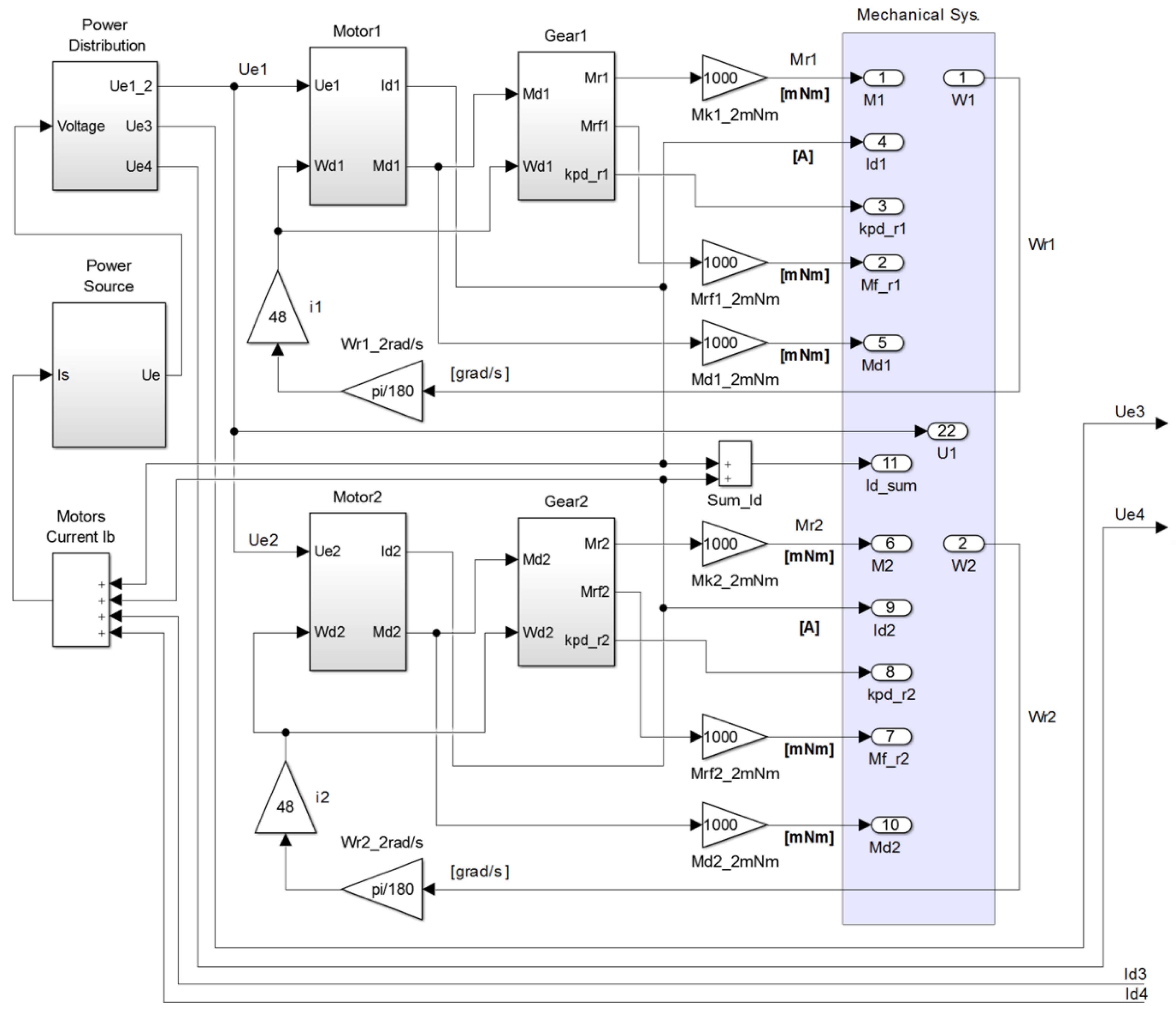
Figure 14 shows the general block diagram of the drive part of the computer model of the MMR transport system.

Since this article considers only the study of the rectilinear locomotion of the MMR with a fixed chassis geometric configuration (i.e., CGV drives are not involved), Figure 14 shows only that part of the model that refers to tractive drives. The model of the drive part of the CGV subsystem has a similar form to that of the tractive drives. Figure 14 shows only the input actions to the CGV drives, designated as Ue3 and Ue4, as well as feedback signals with the values of the motor currents of the front (Id3) and rear (Id4) CGV drives.

The Simulink block diagrams of the models that make up the complete diagram in Figure 14 are shown in Figure A3, Figure A4, Figure A5, Figure A6 and Figure A7 of Appendix B. These diagrams were developed following the mathematical description presented earlier in Section 3.2. The distinctive features of these models discussed above are highlighted with dotted frames in the figures.

3.4.3. Executive Subsystem Model

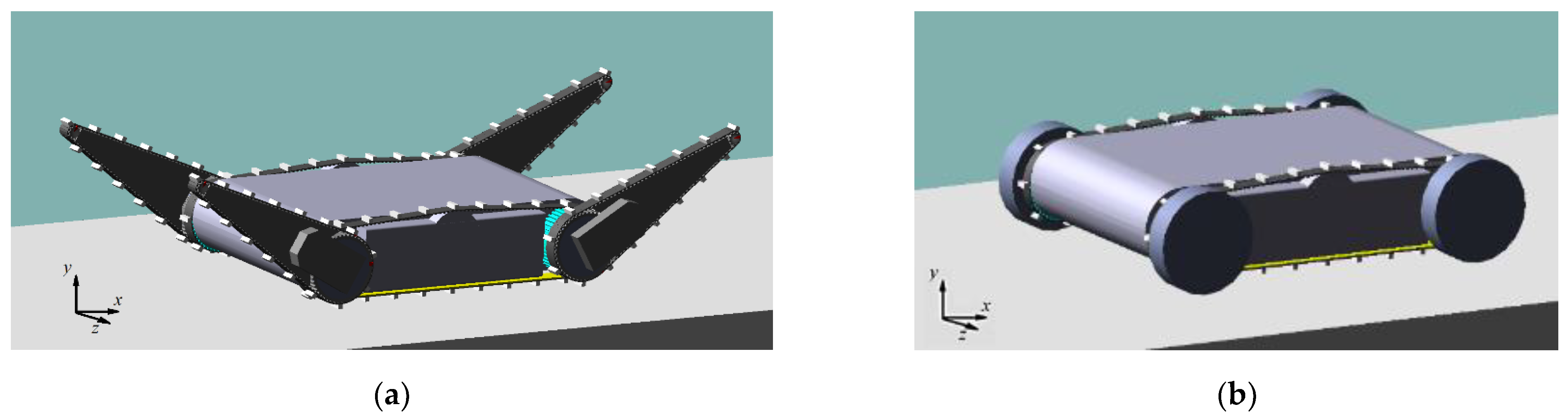
Figure 15 shows the appearance of the simulation computer model of the executive part of the MMR transport system. The model includes the following components:

• The body;
• Two toothed belt drives with grousers, simulating the main tracks of the MMR;
• Four levers (flippers);
• Four toothed belt drives with grousers, simulating additional MMR tracks on the levers in the 6T2A tracked configuration;
• Four wheels simulating the supporting elements in the 4W2T wheeled configuration.

Geometric parameters and relationships between the components of the model correspond to the parameters determined in [37] as a result of the parametric synthesis of the chassis structural–kinematic scheme, based on optimization according to the criterion of minimizing the chassis dimensions while maintaining the specified parameters of geometric traversability (while locomotion on an uneven surface). 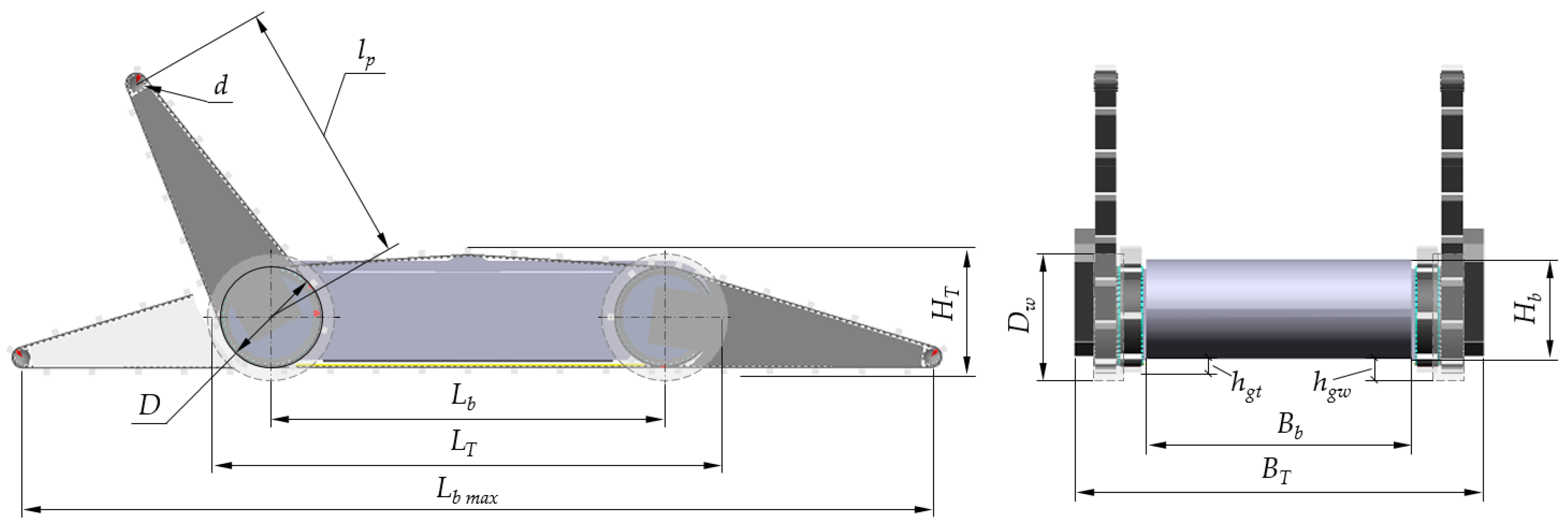Figure 16 demonstrates the geometric characteristics of the MMR transport system.

The main geometric parameters of the transport system model are shown in

Table 6. Geometric parameters of the MMR transport system model (in mm).

Parameter	Designation	Value
Overall length in transport position	LT	390
Overall height in transport position	HT	87.4
Chassis width measured over the tracks	BT	278
Wheel base	Lb	300
Lever length	lp	205
Maximum length of the chassis supporting surface	Lb max	705
Nominal diameter along the middle line of the tracks:
main and additional pulleys	D	87.4
guide rollers	d	27
Wheel diameter	Dw	100
Body height	Hb	76
Body width	Bb	208
Ground clearance in the configuration:
6T2A	hgt	10.7
4W2T	hgw	17

.

The mass–inertial parameters of the model components are set based on the results of the design study in the CAD soft. Determination of the total moment of inertia of the rotating masses $J_S^d$, reduced to the axis of the drive wheel (pulley), is made according to the equation [39]

$$J_S^d=J_d{i}_r^2{\eta }_r+J_w,$$

(31)

where $J_d$ is the inertia of the parts rotating at the same speed as the motor shaft and $J_w$ is the inertia of the parts rotating at the same speed as the drive wheel (pulley).

Table 7. Mass–inertial parameters of the model.

Parameter	Quantity	m [g]	Jz [kg·mm2]	Applicability
				6T2A	4W2T
Main track pulley	2	82	75	+	+
Additional pulley	2	104	140	+	+
Additional rotating parts related to the driving wheel (pulley)	2	0 *	5760	+	+
Wheel	4	86	152	–	+
Lever	4	470	1470	+	–
Main track	2	40	1.59	+	+
Additional track	4	25	1.00	+	–
Body	1	10.3 × 103	1.19 × 105	+	+
Robot in the 6T2A configuration	1	13.1 × 103	2.51 × 105	+	–
Robot in the 4W2T configuration	1	11.5 × 103	1.45 × 105	–	+

* Component weights are taken into account in the body weight.

shows the calculated values of the mass–inertial parameters of the model in the form of masses $m$ of individual components and inertias J_z relative to the axis of rotation (the z-axis that is shown in Figure 15).

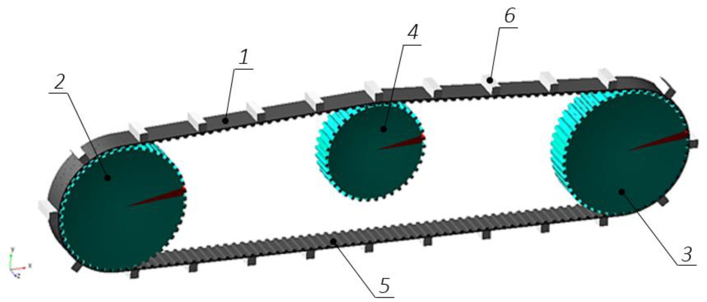
3.4.4. Model of the Chassis Tracked Mover

The essential and most complex part of the model is the model of the track as the flexible body. The construction of the model of the track and the entire tracked mover, following the provisions given in Section 3.2.4, is done in ADAMS. The appearance of the simulation model of the MMR tracked mover is shown in Figure 17.

The chassis tracked mover unit is a belt drive with a toothed belt, driving and driven pulleys, and a tensioner. The main track model in accordance with the diagram of Figure 6 comprises 168 teeth (track elements) and 24 grousers. The additional flippers track model comprises 112 teeth and 16 grousers.

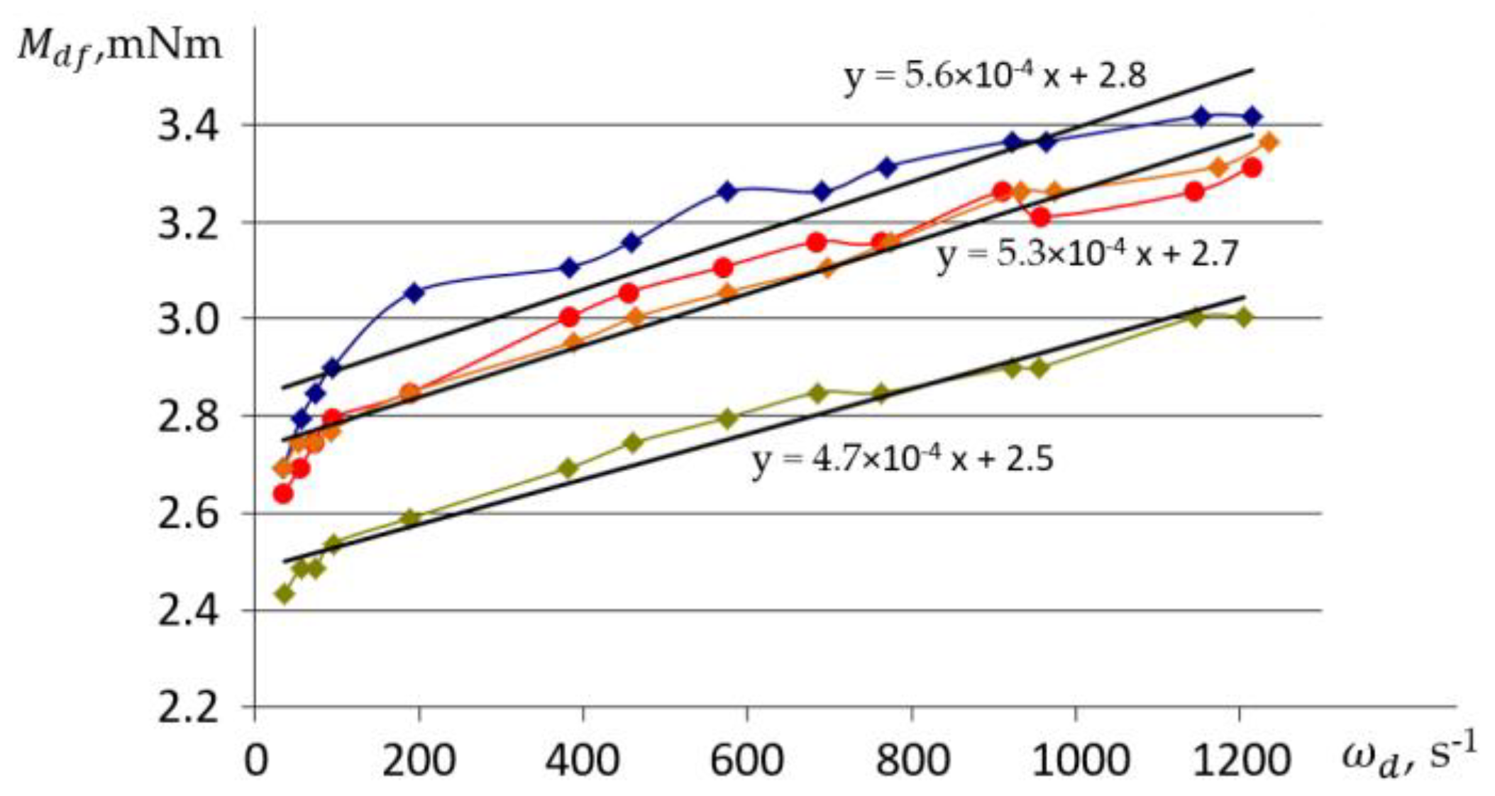
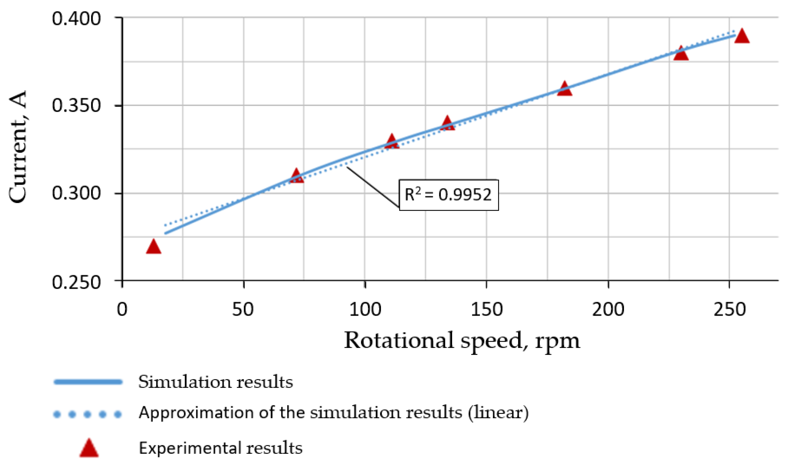
Figure 18 shows the results of comparing the simulated and experimental dependences of the drive motor current in the belt drive on the speed of the drive pulley when rotating at idle. The results of determining the values of the torque of internal resistance $M_{ti}$ in the belt drive confirmed the presence of dependence on speed. This dependence, as shown in Figure 18, is well approximated by a linear characteristic. The reliability of the approximation obtained is characterized by the R² factor equal to 0.995, calculated according to Appendix C.

The high convergence of the results for calculations and experiments demonstrates the adequacy of the belt drive (i.e., tracked mover) model developed, which is the basis for the model of the MMR transport system.

3.4.5. Complete Model of the MMR Transport System

The complete computer (simulating) model combines all the model blocks described above. The simulation itself is carried out in ADAMS, which allows for visualizing the locomotion of the robot and analyzing the characteristics of any components of its transport system.

The complete model of the MMR transport system allows for simulating the general case of the robot’s locomotion, including investigating the power, kinematic, and energy characteristics of the drives when traction drives and CGV drives work together during the dynamic overcoming of obstacles. The most difficult thing, in this case, is simulating the interaction of the chassis of the transport system with the supporting surface and with the body elements of the MMR. The complete model of the chassis in the 6T2A configuration includes a description of 1680 contact interactions.

At the same time, for the particular case of locomotion on a flat surface considered in this article, the complete model can be significantly simplified. The simplified model with excluded unused contacts includes 720 active models of contact interactions of the main tracks with the surface and with the robot body (Figure 6).

The study results of this model are reported further.

3.5. Simulation Experimental Setup

A series of simulation tests were undertaken for the rectilinear locomotion on inclined surfaces of the MMR with a fixed chassis geometric configuration to study the locomotion subsystem of the MMR transport system (i.e., the subsystem of tractive drives). The simulation setup diagram can be seen in Figure 4. Both configurations of the MMR transport system were simulated during these tests: tracked 6T2A and wheeled 4W2T.

The loading mode of the transport system was set by varying three parameters:

• A surface slope angle α;
• MMR mass (imitating the installation of additional weights on MMR platform with the mass of $m_c$);
• Supply voltage of traction motors $U_e$ (i.e., speed-loading mode of the transport system).

The values of the varied parameters are given in

Table 8. The values of the variable parameters in simulations and experimental studies.

Parameter	Slope Angle	Additional Load Mass	Supply Voltage
Designation	α	$m_c$	$U_e$
Units	Degree	kg	V
Set of values	0, 5, 10, 15, 20	0, 1.5, 3, 5, 6.5, 8	15, 24, 33

.

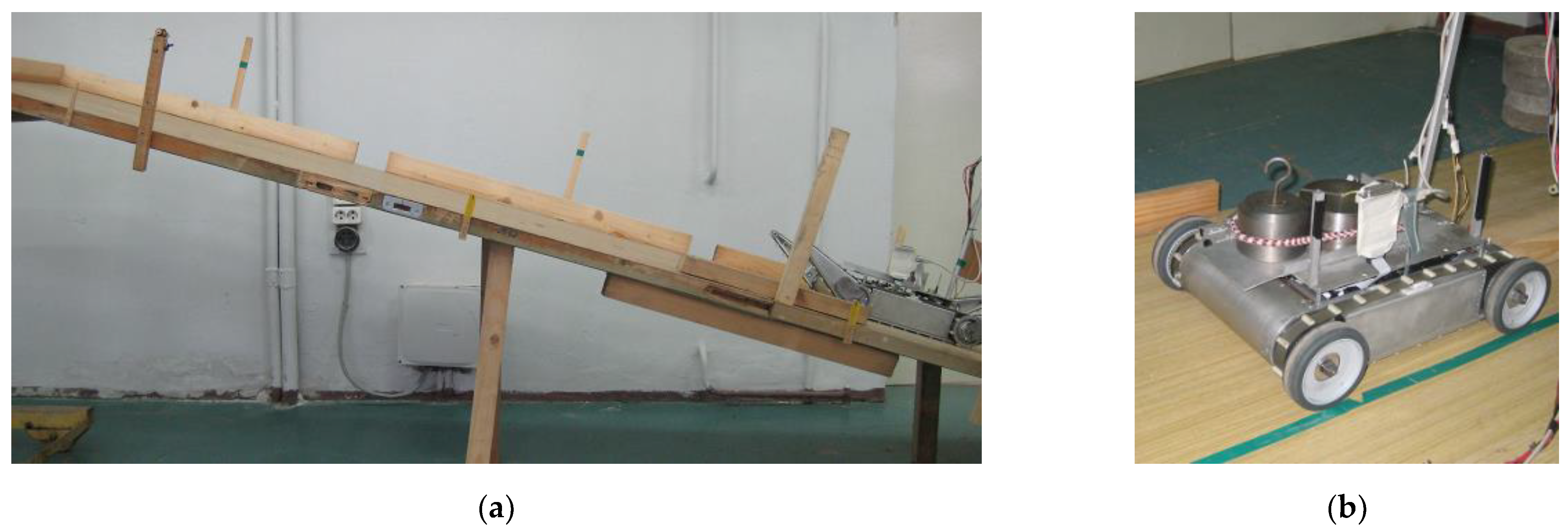
3.6. Physical Experimental Setup

To check the reliability of the simulations, a set of experimental studies was carried out on the MMR mock-up with geometric and mass–inertial parameters corresponding to the computer model developed and by a method similar to virtual experiments.

The force-loading mode of the transport system was set, as shown in Figure 19, by changing the angle of inclination of the surface and installing loads of different mass on the MMR. The speed-loading mode of the transport system was set by setting the required voltage value $U_s$ on the external power source (see Figure A3 of Appendix B).

In order to study the transport system as an electromechanical unit described in Section 2.1, the elements of the MMR on-board control system (OBC) were disconnected from the drives. In this case, the power supply of the electric drives themselves was carried out from an external stabilized power source (EPS), which made it possible to set various voltage values (i.e., to set up speed-loading modes) and control energy consumption directly on the motors. 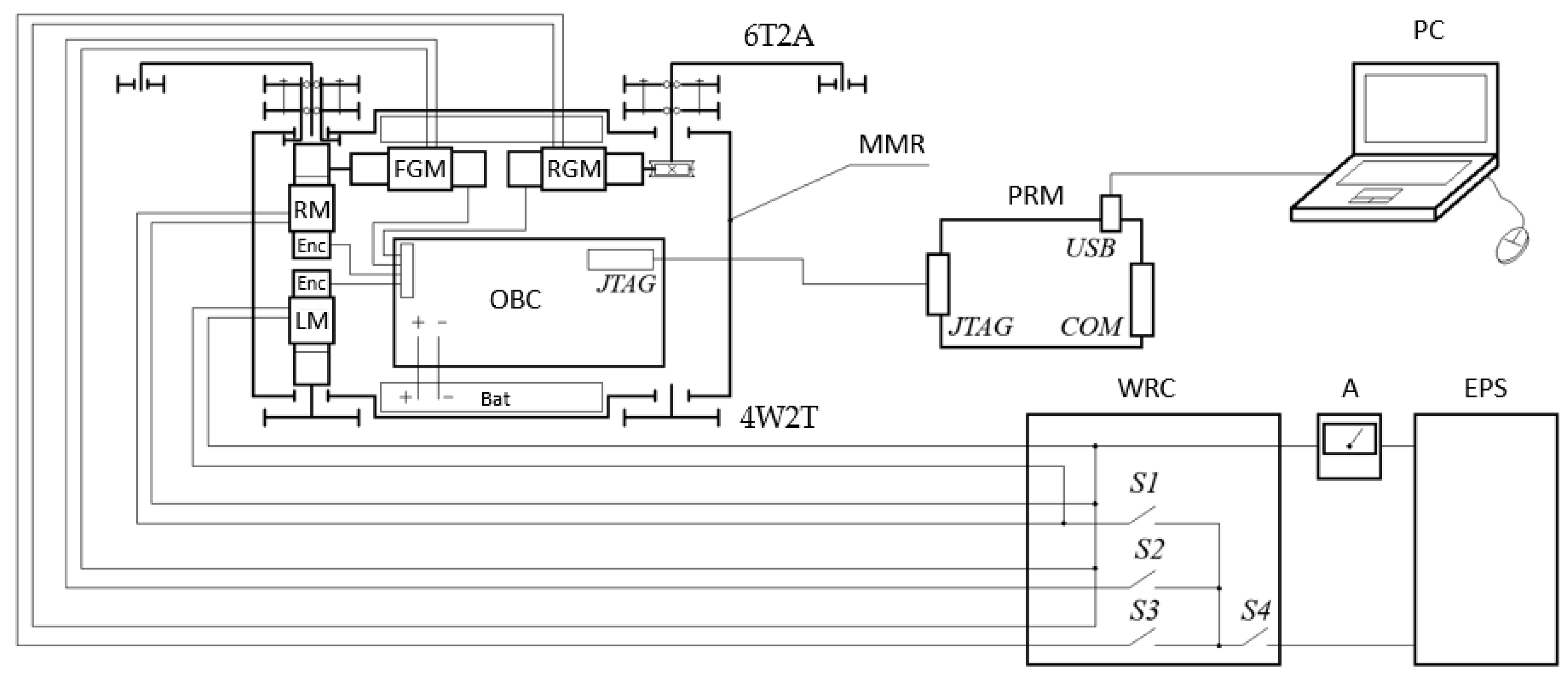Figure 20 shows a diagram of connecting measuring devices to the experimental MMR, and Figure 21 shows the appearance of the connected equipment.

The motor rotational speed measurement was carried out using the programmer of the 56F800E family controllers, which was used to read the readings directly from the encoders of the motors through the JTAG interface available on the OBC board. The programmer was fixed on the MMR and connected to a portable PC via a USB interface.

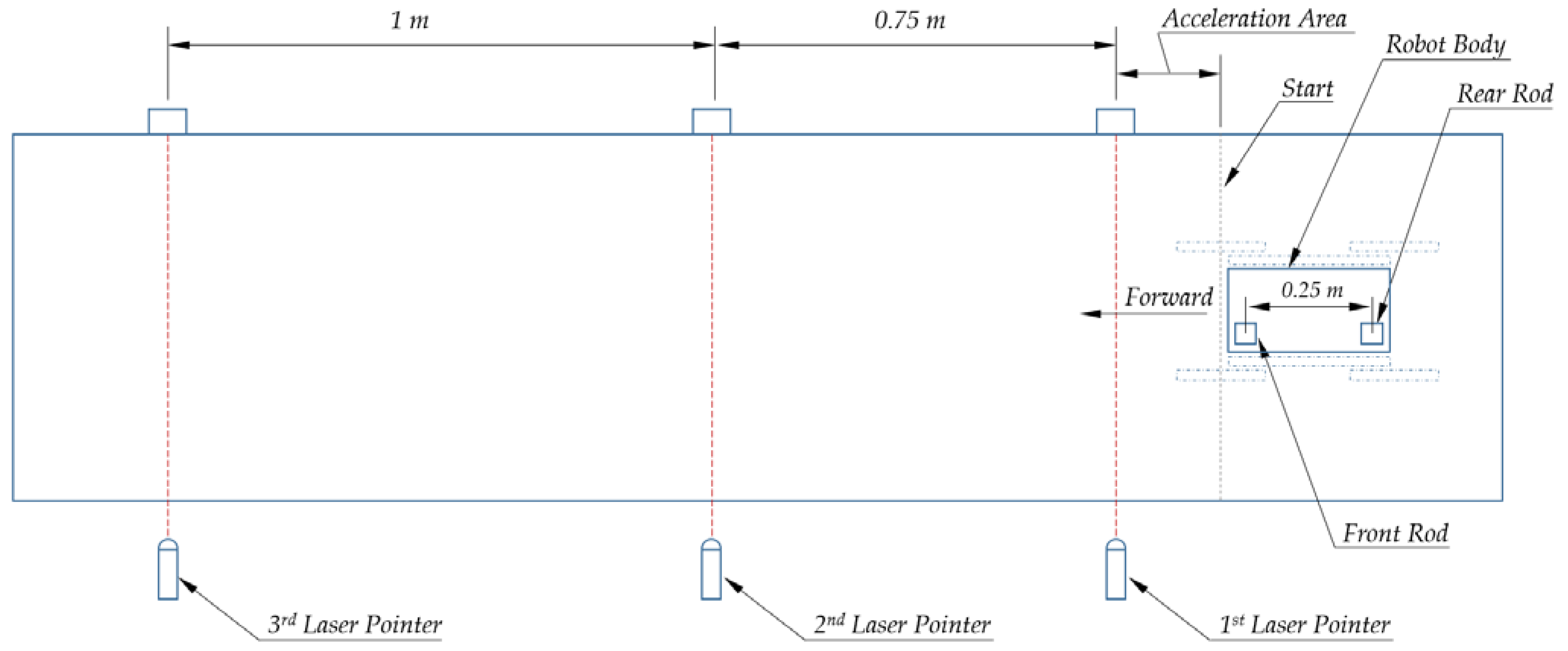
The measurement of the MMR actual linear speed was carried out by measuring the time between sequential interruptions of optical beams from three laser pointers, installed along the test bench at certain distances from each other, by two rods mounted on the robot in front and rear. The schematic of such measurements is shown in Figure 22. Therefore, the robot motion is accompanied by a six-fold interruption of the laser beams. From the known distances between the laser pointers and between the rods on the robot body, it becomes possible to determine the actual average speed of the robot. To exclude the influence on the result of the stage of acceleration, the MMR was installed so that the acceleration was completed by the time of the first laser beam was crossed. The robot path length during the steady-state motion was 2 m. Video recording of the MMR locomotion was carried out during all tests.

The test surface of the test bench corresponds to the surface of “type 3” by Table 5, characterized by a low value of the adhesion coefficient ${\phi }_x$, which makes it possible to study the robot slipping effects during its locomotion on the inclines.

During the experimental studies, the following characteristics were directly measured:

• Total motor consumption $I_{\Sigma }$ (using ammeter, see Figure 20);
• Frequencies of rotation of the motors $n_{di}$ (using the programmer device, see Figure 20);
• Actual linear speed $V_x$ (using the method described above).

The theoretical robot speed $V_{x\_teor}$ and energy consumption in each of the MMR transport system components were indirectly determined.

Thus, the experimental procedure of the rectilinear motion study of the MMR transport system was as follows:

• Connect the measuring equipment to the MMR following Figure 20 (if necessary);
• Set the required value of the surface slope angle (following Table 8);
• Set on the MMR required additional load mass (following Table 8);
• Set the required voltage value on the external power source (following Table 8);
• Set the MMR to the starting position;
• Check the required current measurement range of the ammeter;
• Turn on the recording by PC of the motor rotation frequencies (see Figure 20);
• Enable video recording of the MMR locomotion;
• Set the forward movement of the MMR by turning on switches S1 and S4 of the WRC (see Figure 20);
• Turn off switch S4 when the MMR reaches the endpoint of the path;
• Stop recording the motor rotation frequency and video recording;
• Enter in the experimental data log information about the test mode (voltage, slope angle, additional load mass) and the corresponding file names;
• Repeat measurements following points 5 to 12 at least three times;
• Analyze the files received. The measurement results of the total energy consumption, the average rotational frequencies of the motors, and the average speed of the MMR at steady-state stage are averaged by the number of attempts and entered in the table of research results.

4. Results

4.1. Simulation Study

This article considers the results of simulation of a particular case of the MMR transport system locomotion, namely, locomotion on surfaces with different angles of inclination. This mode is a traditional widespread analytical case in the theory of transport vehicle design [10,11,12,14,17,19,20,34,35,40], allowing for the study of the traction–adhesion properties of the terrain-vehicle system in various drive conditions.

The purpose of the transport system simulation is to study the processes of acceleration and steady-state locomotion at various loading modes, and to determine the effective values of the loads on the transport system elements and its energy consumption for movement, as well as to determine the nature of the influence on these values by the current angle of inclination of the surface and the total weight of the robot, i.e., to estimate the carrying capacity of the MMR transport system.

The specified test conditions include the angle of inclination of the surface, the mass of the additional load (i.e., the total mass of the robot, taking into account the additional load), the speed-loading mode (the drives supply voltage), and the type of locomotion surface.

As the surface in this study, a test surface with relatively low adhesion properties was used (a surface type 3 according to Table 5, with adhesion coefficient equal to about 0.32 to 0.35), which made it possible to study, among other things, the modes of locomotion with slipping (skidding) of the transport system movers.

A universal characteristic of the energy consumption of drives is the total consumed current I_Σ of the motors. Figure 23 shows typical graphs of the total current for two transport system options: six-track 6T2A and four-wheeled 4W2T. These graphs were obtained for the case of the transport system locomotion on a horizontal surface with a power supply voltage of 33 V. The graphs obtained under other simulated conditions (other voltage, different angles of inclination of the surface, the presence of a payload) have a similar appearance.

Three zones are clearly distinguishable on the graphs, which characterize the following stages of locomotion: I—starting, II—acceleration with slipping, and III—uniform (steady-state) of the locomotion. The slippage presence is indicated by increased consumption in zone II, i.e., the presence of additional energy losses, as well as a comparison of the graphs of the real (actual) robot speed $V_x$ and its theoretical speed $V_{x\_teor}$, determined by the wheel speed in accordance with the equation

$$V_{x\_teor}=\frac{{\sum }_{i=1}^n{\dot{\phi }}_{ki} }{n} r_k,$$

(32)

where ${\phi }_k$ is the wheel rotation angle of the i-th drive; $r_k$ is the wheel/pulley rolling radius; n is the supporting wheels/pulleys number.

A comparison of the $V_x$ and $V_{x\_teor}$ graphs obtained for the same test conditions as the graphs in Figure 23 is shown in Figure 24.

The degree of slipping over the time interval $t^{\prime }$ is determined by the slippage [10,19,34,40,50]:

$$s=1-V_x/V_{x teor}$$

(33)

The graphs of $I_{\Sigma }$, $V_x$, and $V_{x\_teor}$ at steady-state are characterized by significant fluctuations, especially explicit for the 6T2A tracked option (these fluctuations are not noticeable for the 4W2T option on the scale of Figure 23 and Figure 24 since they have an order of magnitude smaller amplitude). The graphs of the total energy consumption during steady-state according to Figure 23 are enlarged in Figure 25.

The analysis of the simulation results for the 6T2A option shows that these fluctuations are caused by the uneven movement of the tracks, and their period exactly matches the pitch $S_g$ of the grousers (see Figure 6), and is determined by the equation

$$T_{s_i}=\frac{S_g}{{\dot{\phi }}_{ki}{r}_k}.$$

(34)

Equation (34) is also valid for the 4W2T option if the pitch of the working teeth $S_t$ is inserted instead of $S_g$.

The reason for more significant fluctuations for the tracked option 6T2A is in the nature of the interaction of the mover with the surface. The pattern of this interaction is different for tracked and wheeled chassis. For the wheeled chassis option, the interaction of the movers with the surface occurs through four supporting points and the main tracks play the role of only transmission mechanisms, not loaded with normal reactions. For the tracked chassis option, each track, as shown in Figure 26, interacts with the surface through the grousers, further transferring these loads to the front and rear pulleys and lower guides. At the same time, the joint analysis of animations and graphs obtained during the simulation (Figure 26) shows that the peaks of current fluctuation occur at the moments of impacts of the grousers that are currently incoming into contact with the surface (highlighted in Figure 26 with the red circle). The oscillations of the wheel speeds and the robot linear speed are also associated with this. However, as a result of the assessment, it is found that the amplitude of these fluctuations does not exceed 2%.

The described nature of the interaction is confirmed by the graphs of normal reactions on one side of the chassis, as shown in Figure 27. For the 6T2A option, there are significant fluctuations in the total reaction associated with the interaction of the grousers with the surface and the working teeth of the track with the lower guide. The entry and exit of each grouser from engagement with the surface is accompanied by a peak of normal reaction. For the 4W2T option, the oscillations are much less explicit and their amplitude is more than two orders of magnitude smaller.

4.2. Experimental Studies and Model Verification

To verify the reliability of the computer simulation results, a set of experimental studies was performed on the MMR mock-up with geometric and mass inertia parameters corresponding to the computer model developed and using a technique similar to the virtual experiments performed.

Figure 28 shows the results of measurements of the total motor consumption I_Σ at various loading modes of the transport system.

As is shown in Figure 28, the experimental data are well approximated by linear dependencies that are confirmed by the corresponding R² values calculated according to Appendix C.

Table A1. Experimental and simulated data obtained during rectilinear locomotion of the 6T2A option.

Test Conditions				Experimental Data			Simulating Data			Data Discrepancies
${\mathit{U}}_{\mathit{e}}$ [V]	${\mathit{M}}^{ *}$ [kg]	${\mathit{m}}_{\mathit{c}}$ [kg]	$\mathit{\alpha }$ [°]	${\mathit{I}}_{\mathsf{\Sigma }}$ [A]	${\mathit{n}}_{\mathit{d}\mathit{i}}$ [rpm]	${\mathit{V}}_{\mathit{x}}$ [mm/s]	${\mathit{I}}_{\mathsf{\Sigma }}^{\mathit{s}}$ [A]	${\mathit{n}}_{\mathit{d}}{}^{\mathit{s}}$ [rpm]	${\mathit{V}}_{\mathit{x}}{}^{\mathit{s}}$ [mm/s]	$\mathit{\delta }{\mathit{I}}_{\mathsf{\Sigma }}$ %	$\mathit{\delta }{\mathit{n}}_{\mathit{d}}$ %	$\mathit{\delta }{\mathit{V}}_{\mathit{x}}$ %
15	13.1	0	0	2.30	4930	420	2.22	5170	431	–3.6	+4.6	+2.6
			5	2.75	4800	400	2.67	5100	422	–3.0	+5.9	+5.2
			10	3.00	4745	390	3.10	5030	413	+3.3	+5.7	+5.6
			15	3.45	4625	375	3.55	4960	402	+2.8	+6.8	+6.7
			20	3.85	4560	360	3.92	4880	385	+1.8	+6.5	+6.5
33	21.1	8	0	3.20	11,590	970	3.01	11,830	985	–6.3	+2.0	+1.5
			5	4.00	11,340	920	3.76	11,640	961	–6.4	+2.6	+4.3
			10	4.60	11,170	900	4.50	11,670	951	–2.2	+4.3	+5.4
			15	5.25	11,070	860	5.09	11,490	899	–3.1	+3.7	+4.3
			20	5.85	10,900	780	5.95	11,410	829	+1.7	+4.5	+5.9

* M is the robot mass.

and

Table A2. Experimental and simulated data obtained during rectilinear locomotion of the 4W2T option.

Test Conditions				Experimental Data			Simulating Data			Data Discrepancies
${\mathit{U}}_{\mathit{e}}$ [V]	${\mathit{M}}^{ *}$ [kg]	${\mathit{m}}_{\mathit{c}}$ [kg]	$\mathit{\alpha }$ [°]	${\mathit{I}}_{\mathsf{\Sigma }}$ [A]	${\mathit{n}}_{\mathit{d}\mathit{i}}$ [rpm]	${\mathit{V}}_{\mathit{x}}$ [mm/s]	${\mathit{I}}_{\mathsf{\Sigma }}^{\mathit{s}}$ [A]	${\mathit{n}}_{\mathit{d}}{}^{\mathit{s}}$ [rpm]	${\mathit{V}}_{\mathit{x}}{}^{\mathit{s}}$ [mm/s]	$\mathit{\delta }{\mathit{I}}_{\mathsf{\Sigma }}$ %	$\mathit{\delta }{\mathit{n}}_{\mathit{d}}$ %	$\mathit{\delta }{\mathit{V}}_{\mathit{x}}$ %
15	13.1	0	0	0.66	5410	590	0.66	5455	595	+0.5	+0.8	+0.8
			5	1.14	5090	550	1.18	5398	587	+3.4	+5.7	+6.3
			10	1.60	5000	550	1.71	5339	579	+6.4	+6.3	+5.0
			15	2.10	4970	540	2.20	5274	571	+4.5	+5.8	+5.4
			20	2.55	4810	520	2.72	5128	552	+6.3	+6.2	+5.8
33	21.1	8	0	0.84	12,270	1340	0.81	12,075	1318	–3.7	–1.6	–1.7
			5	1.76	11,920	1295	1.67	11,978	1305	–5.4	+0.5	+0.8
			10	2.44	11,730	1270	2.56	11,880	1289	+4.7	+1.3	+1.5
			15	3.40	11,490	1220	3.44	11,778	1267	+1.2	+2.4	+3.7
			20	4.20	11,230	1180	4.29	11,685	1241	+2.1	+3.9	+4.9

* M is the robot mass.

of Appendix D show the experimentally determined values of $I_{\Sigma }$, $n_{di}$, and $V_x$, obtained during the rectilinear steady-state locomotion of the MMR transport system in configurations 6T2A and 4W2T for two loading modes. The first mode is the mode of conditionally minimum load characterized by a supply voltage $U_e$ of 15 V and zero payload $m_c$. The second mode is the conditionally maximum load characterized by a supply voltage $U_e$ of 33 V and a maximum payload $m_c$ of 8 kg.

The identity of the virtual and physical experiments performed allows for comparing their results. In the course of this comparison, the discrepancies between the simulated and experimental data, $\delta CV$ (i.e., simulating error), for those parameters that were determined directly ($I_{\Sigma }$, $n_{di}$, $V_x$) were estimated using the equation

$$\delta CV=\frac{CV-EV}{CV}\cdot 100\%,$$

(35)

where $\delta CV$ is the calculated error of the CV; $CV$ is the simulated value; $EV$ is the experimental value.

These simulation errors are also presented in Table A1 and Table A2 of Appendix D.

Comparison of experimental and simulated data showed their close convergence in the range of $\delta CV$ discrepancies not exceeding 5 to 7%, which allows for confirming the validity of the approaches proposed in the construction of the computer model and the adequacy of the MMR’s transport system model, which has a fairly accurate correspondence to its physical prototype.

5. Discussion

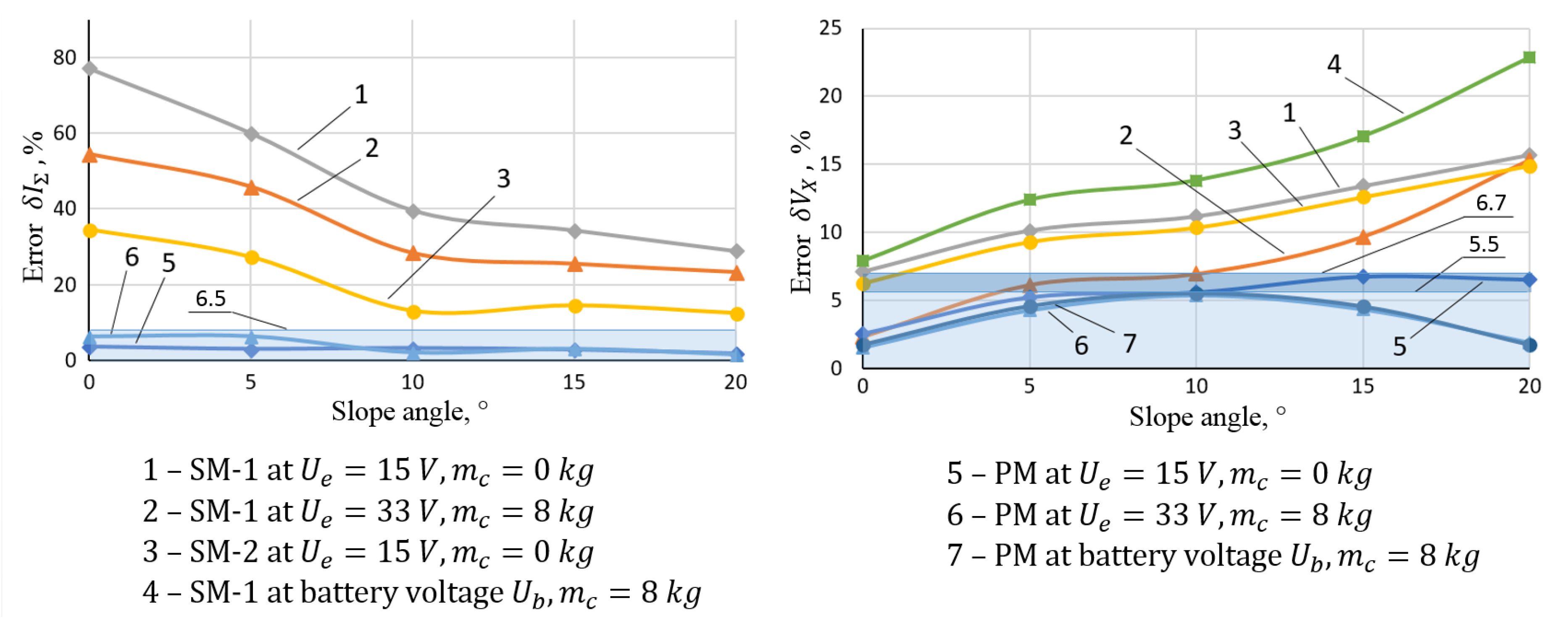
The computer model developed for the MMR transport system was compared with simplified models that do not take into account the features of the mathematical description given in Section 3.2. This was necessary to assess the significance of the proposed approaches. Figure 29 shows the comparative analysis results of three model options: the proposed model (PM) and two versions of simplified models (SM-1 and SM-2).

In comparison with the detailed PM-model, the simplified SM-models are distinguished by the use of constant values of the internal friction characteristics of motors and reduction gears. The difference between SM-1 and SM-2 is the different value of the internal resistance in the tracks, which also does not depend on speed in simplified models. A brief description and the main parameters of the compared models are presented in

Table A3. Brief description of the compared models.

Characteristics	Proposed Model (PM)	Simplified Model 1 (SM-1)	Simplified Model 2 (SM-2)
Torque of internal resistance forces of the motor $M_{df}$	$M_{df}=f\left({\dot{\phi }}_d\right)$ see (14)	$M_{rf}=const\left({\dot{\phi }}_d\right)$	$M_{rf}=const\left({\dot{\phi }}_d\right)$
Total torque of gear internal resistance $M_{rf}$	$M_{rf}=f\left(M_d, {\dot{\phi }}_d\right)$ see (20),(22)	$M_{rf}=f\left(M_d\right)$ see (21)	$M_{rf}=f\left(M_d\right)$ see (21)
Gear efficiency ${\eta }_r$	${\eta }_r=f\left(M_r, {\dot{\phi }}_r\right)$ see (19),(20)	${\eta }_r=const$	${\eta }_r=const$
Torque of internal resistance forces in the track $M_t$	$M_t=f\left(\dot{{\phi }_k}\right)$, see (24)	$M_t=const$ $M_t\approx 1/3\cdot M_{t0}$	$M_t=const$ $M_t\approx M_{t0}$
External power supply voltage $U_s$ ($U_s=U_e$)	$U_s=const$	$U_s=const$	$U_s=const$
On-board battery voltage $U_b$	$U_b=f\left(I_s, I_p, U_{b0}\right)$ see (10)–(13)	$U_b=U_{b0}=const$	$U_b=U_{b0}=const$

and

Table A4. Main parameters values of the compared models.

Parameter	Designation	Unit	PM	SM-1	SM-2
Static motor friction torque	$M_{df0}$	mNm	2.7	4.2	4.2
Motor viscous friction coefficient	$K_{fd}$	mNm·s	5.5 × 10−4	–	–
Gear friction torque measured on the gear’s input shaft	$M_{rf0}$	mNm	0.3	–	–
Gear coefficient of viscous friction	$K_{fr}$	mNm·s	1.4 × 10−3	–	–
Gear efficiency	${\eta }_r$	–	see (19)	0.75	0.75
Static torque of the internal friction forces of the tracked unit of the one side of chassis (three tracks)	$M_{t0}$	mNm	350	108	300
Coefficient of pseudo viscous friction in the tracked unit of the one side of chassis (three tracks)	$K_{ft}$	mNm·s	16	–	–
Friction coefficient of the track along the guide of the robot body	${\mu }_t$	–	0.20	0.20	0.20
Coefficient of motion resistance (tracked chassis)	$f_t$	–	0.06	0.06	0.06
Coefficients of longitudinal adhesion (chassis mover-surface)	${\phi }_x$	–	according to Table 5	according to Table 5	according to Table 5
No-load battery voltage	$U_{b0}$	V	33.4	33.6	33.6
Total current from all other MMR consumers, not related to the transport system	$I_p$	A	1.5	–	–
Battery total self-electric resistance	$R_b$	Ohm	0.4	–	–
Battery cell experimental parameters	$A$	–	7 × 10−8	–	–
	$B$	–	–5 × 10−4	–	–

of Appendix D.

Figure 29 shows the simulation results of the rectilinear locomotion of the MMR in the 6T2A chassis configuration up inclined surfaces as the test scenario. In order to assess the effect of various loading options (speed- and force-loading modes) in greater detail, the simulations were performed in two distinctive modes, which contingently corresponded to the minimum and maximum loads: (1) at a supply voltage $U_e$ of 15 V and zero payload mass $m_c$ and (2) at $U_e$ = 33 V and $m_c$ = 8 kg. The case of supplying from an on-board power source was also studied (see curves 4 and 7 in Figure 29).

The calculation errors of the total current consumption of the drives $\delta I_{\Sigma }$ (Figure 29, left side) and the linear speed $\delta V_x$ (Figure 29, right side), defined by Equation (35), were accepted as the estimated parameters for comparison. In addition to the payload mass $m_c$, the force-loading mode was also set by changing the slope angle $\alpha$, which is an independent axis in the graphs shown in Figure 29.

The data of Figure 29 show that the errors obtained using simplified models (curves 1–4) significantly exceed the errors obtained using the proposed detailed model (curves 5–7).

An evaluation of the convergences of the experimental data and the simulated data obtained using the PM-model and the simplified SM-models shows that the proposed approaches to computer model development can increase the accuracy of simulations (as a difference in the calculated errors) by 10 to 25% at maximum loading modes, and up to 30 to 70% at low and medium loading modes.

6. Conclusions and Future Work

This work is devoted to the study of electromechanical systems of locomotion of small-sized (portable-type) mobile robots. As shown in the study, taking into account internal losses (i.e., friction) in all components plays a significant role for these robots. Another important point is the relatively high mobility (as locomotion speeds) of these robots. Therefore, it is important to take into account not only the force-loading mode, but also the speed-loading mode (i.e., a significant dependence of the friction forces on speed) when simulating transport systems of such high-speed and small-sized mobile robots.

The proposed simulation method includes the following items and features described in the corresponding sections of this article:

• Use of models of internal resistances in the form of dependences on speed for all mechanical components of the transport system: motors in the form (14), gearboxes in the form (20) and (22), and tracks in the form (24);
• Use of the battery model, taking into account the total current load from all consumers within the robot and the current state of charge of the battery in the forms of Equations (11)–(13);
• Use of the track model in accordance with Figure 6 to simulate it as a flexible part that is a source of oscillations during a robot motion;
• Use of models of contact interactions described in Section 3.2.4;
• Use of experimentally determined parameters from the above models (Table 1, Table 2, Table 3, Table 4 and Table 5);
• Use of geometrical and mass–inertial parameters of MMR corresponding to its physical model (Table 6 and Table 7);
• Structural and functional division of the computer model into two interacting parts following Figure 13—a model of the drive subsystem and a model of the executive subsystem, which allows for simulating not only the simplest case of locomotion on inclined flat surfaces considered in this article, but also for more complex scenarios, including overcoming obstacles.

The article shows what the computation errors can be when applying the approaches used in automobile and tractor design theory, as well as in larger robot design, to small-sized transport systems of portable-type mobile robots. Thus, the results of the comparative simulation show that when simplifying the models, the calculated errors can reach up to 25% at maximum (i.e., nominal) load modes, and up to 70% at partial load modes. This shows that neglecting the proposed approaches to simulating the transport systems of the MMRs leads to results that are not applicable from a practical point of view. At the same time, the article shows the attainable level of computation error obtained, which in this study was no more than 7% in the entire range of load modes.

The main contribution of this article is aimed to an increase in the efficiency of design work on the development of highly mobile small-sized ground robots, due to increasing the accuracy of dynamic calculations of their locomotion subsystems.

The approaches proposed in this article make it possible to create a simulating model of the MMR transport system with a high degree of adequacy to the experimental model. The results of the study can be used to build computer models of small-sized mobile robots to study their operating modes, both at the stage of robot development and at the stage of assessing the characteristics and critical operating modes of an existing robot.

The authors connect the further development of this work with the following key areas:

• Development and experimental verification of a complete computer model of a small-sized mobile robot on basis of proposed approaches for the composition of the transport system model, with the addition of a model of a control system for mobile robot executive subsystems, i.e., a transport subsystem and a functional subsystem (i.e., manipulators, technological equipment, etc.).
• Research and study ways to create an adaptive control system for a mobile robot that can increase its stability of motion at high speeds, as well as timely detect and fend off critical situations that can lead to robot malfunction or breakdown.