Article

A Self-triggered Position Based Visual Servoing Model Predictive Control Scheme for Underwater Robotic Vehicles †

by
Shahab Heshmati-alamdari
1,
Alina Eqtami
2,
George C. Karras
3,4,
Dimos V. Dimarogonas
1 and
Kostas J. Kyriakopoulos
4,*
1
Division of Decision and Control Systems, School of Electrical Engineering and Computer Science, KTH Royal Institute of Technology, SE-100 44 Stockholm, Sweden
2
Laboratoire des Signaux et Systémes (L2S) CNRS, CentraleSupélec, Université Paris-Sud, Université Paris-Saclay 3, rue Joliot-Curie, 91192 Gif-sur-Yvette, CEDEX, France
3
Department of Computer Science and Telecommunications, University of Thessaly, 3rd Km Old National Road Lamia-Athens, 35100 Lamia, Greece
4
Control Systems Laboratory, School of Mechanical Engineering, National Technical University of Athens, 15780 Athens, Greece
*
Author to whom correspondence should be addressed.
This paper is an extended version of our paper published in Shahab Heshmati-Alamdari, Alina Eqtami, George C. Karras, Dimos V. Dimarogonas, and Kostas J. Kyriakopoulos. A Self-triggered Visual Servoing Model Predictive Control Scheme for Under-actuated Underwater Robotic Vehicles. In Proceedings of the 2014 IEEE International Conference on Robotics and Automation (ICRA), Hong Kong, China, 31 May–7 June 2014.
Machines 2020, 8(2), 33; https://doi.org/10.3390/machines8020033
Submission received: 1 May 2020 / Revised: 4 June 2020 / Accepted: 7 June 2020 / Published: 11 June 2020
(This article belongs to the Special Issue Intelligent Mechatronics Systems)

Abstract

:
An efficient position based visual sevroing control approach for Autonomous Underwater Vehicles (AUVs) by employing Non-linear Model Predictive Control (N-MPC) is designed and presented in this work. In the proposed scheme, a mechanism is incorporated within the vision-based controller that determines when the Visual Tracking Algorithm (VTA) should be activated and new control inputs should be calculated. More specifically, the control loop does not close periodically, i.e., between two consecutive activations (triggering instants), the control inputs calculated by the N-MPC at the previous triggering time instant are applied to the underwater robot in an open-loop mode. This results in a significantly smaller number of requested measurements from the vision tracking algorithm, as well as less frequent computations of the non-linear predictive control law. This results in a reduction in processing time as well as energy consumption and, therefore, increases the accuracy and autonomy of the Autonomous Underwater Vehicle. The latter is of paramount importance for persistent underwater inspection tasks. Moreover, the Field of View constraints (FoV), control input saturation, the kinematic limitations due to the underactuated degree of freedom in sway direction, and the effect of the model uncertainties as well as external disturbances have been considered during the control design. In addition, the stability and convergence of the closed-loop system has been guaranteed analytically. Finally, the efficiency and performance of the proposed vision-based control framework is demonstrated through a comparative real-time experimental study while using a small underwater vehicle.

1. Introduction

Vision-based control has been extensively investigated in recent decades for the operation of autonomous underwater vehicles [1,2]. Complex underwater missions, such as surveillance of underwater oil/gas pipelines [3,4,5], inspection of underwater communication cables [6,7], and search for hazardous materials (e.g., naval mines) [8,9,10], require detailed and continuous visual feedback, which can be obtained from either monocular or stereo vision systems.
In general, the visual servoing can be categorized in (i) Position-Based Visual Servoing (PBVS), where the visual features extracted along with the help of the visual tracking algorithm are used for the estimation of the three-dimensional (3D) relative position between the camera and visual target; (ii) Image-Based Visual Servoing (IBVS), where the error function is defined directly on the position of the image features in the image plane between the current and desired images [11]; and, (iii) 2-1/2 Visual Servoing, where the error function is partially formulated in both the Cartesian and the image plane. More information regarding the standard visual servoing techniques can be found in the literature [12,13,14]. Regarding visual servo control in underwater robotics, some previous work for the pipe inspection task (for example, oil platforms) were realized in [15,16]. In [17], visual servoing using the Laser Vision System (LVS) combined with an on-line identification mechanism has been investigated and verified experimentally. In [18,19], stereo vision frameworks have been investigated for underwater operation. The docking of underwater robots employing visual feedback has been addressed in [20,21]. Some applications of visual servoing for station keeping of autonomous underwater vehicles are given in [22,23,24].
The control of an underwater vehicle is generally a highly non-linear problem [25,26]. Conventional control strategies, such as input-output decoupling and local linearization [27,28], Output feedback linearization [29,30,31], and combined frameworks involving Lyapunov theory and backstepping have been investigated in the past for the design of motion controllers for autonomous underwater vehicles. However, most of the aforementioned control strategies yield low closed-loop performance and often demand very precise dynamic parameters, which, in most cases, is quite difficult to obtain [32,33]. Moreover, the effect of ocean currents is either assumed to be known or an exponential observer is adopted for its estimation, thus increasing the design complexity [34]. In addition, by employing all of the aforementioned control strategies, it is not always straightforward to incorporate operational limitations (i.e., visual and/or kinematic constraints) into the vehicle’s closed-loop system [35]. In this spirit, the efficient controlling of underwater robotic vehicles continues to pose significant challenges for control designers in view of the numerous limitations and constraints that arise from the nature of the underwater environment [36]. In particular, AUVs are characterized by constrained high-dimensional non-linear dynamics, especially in the case of underactuated systems [37], which induce significant complexity regarding model uncertainty as well as various operational constraints, such as sensing capabilities and visibility constraints [38,39]. In this context, Non-linear Model Predictive Control (N-MPC) [40], is a proper control approach that is to be used in complex underwater visual servoing missions due to its efficient ability to handle input and state constraints. In a vision based MPC setup, the filed of view limitations could be integrated as state constraints [41]. In this spirit, vision based MPC controller have been employed in medical application [42], as well as for navigation of autonomous aerial vehicles [43] and mobile robots [44]. Furthermore, a vision based terrain mapping-model predictive control approach for autonomous landing of an UAV in unknown terrain is given in [45]. In [46], a vision based approach for path following of an omni-directional mobile robot using MPC is presented.
In a typical vision-based control setup, at every sampling time, the visual feedback that is extracted from the image is used for the generation of a proper error [47]. This requires the selection and extraction of appropriate image features and matching them with the corresponding features in the desired image [48]. This process is usually referred in the literature as Visual Tracking [49,50]. Accuracy and robustness are the main concerns of a Visual Tracking Algorithm (VTA) [51]. However, it is known that the accurate and robust VTA in real-time robotic applications is a very heavy process that demands high computational cost [52]. The latter will result in large energy consumption and might cause delays in the closed-loop system. The aforementioned issues become more apparent in the case of small autonomous robotic vehicles (e.g., UAVs, AUVs), where they are usually equipped with a weak computing unit and, in most cases, suffer from limited energy resources and their recharging procedure is difficult and time and cost consuming [53]. On the other hand, in a N-MPC setup, a constrained Optimal Control Problem (OCP) must be solved at each sampling time. The latter is usually considered to be a very computationally demanding task. In addition, these systems are usually equipped with weak computing units that need to solve the VTA and the OCP of the NMPC at each time instant. This usually results in the reduction of the system accuracy, as bigger sampling times are required. Here, the problem is to design an automatic framework that relaxes the rate of control input calculations and visual tracking activation while maintaining the efficiency of the system. In other words, an automatic visual servoing framework that determines when the system requires tracking the visual data and calculating new control inputs while maintaining system performance at the desired level. This encourages the design of a self-triggered visual servoing strategy that is addressed in this work.

1.1. The Self-Triggered Control Framework

Nowadays, periodic control is the standard control framework that is used in most applications. Quite recently, though, a novel formulation of control schemes in a self-triggered manner is becoming popular. The key idea behind the self-triggered control is that the execution of the control task is not made ad-hoc at every sampling time, but, instead, it uses system feedback in order to sample as infrequently as possible while guaranteeing to preserve the stability of the system, see Figure 1. Consequently, this results in an aperiodic sampling system, while also preserving the system performance and stability. In particular, the self-triggered strategy leads to reducing the number of sampling data from the system, a feature that is important and desirable in a various number of applications with operational limitations in sensing, energy, and communication.
The self-triggered control framework along with a closely related framework, named event-triggered control, comprise the recently introduced event-based control framework. Both approaches, self and event-based control, are comprised, inter alia, by a feedback control framework that calculates the control input and a triggering mechanism that decides when the new control update should occur. However, these frameworks are different; the event-triggered control is more reactive with respect to the self-triggered control, as control inputs in this strategy are calculated when the robot state deviates more than a certain threshold from a desired value, while the self-triggered framework can be considered to be proactive, as it computes the next control input ahead of time. Notice, that, in the event-triggered framework, a constant measurement of the system state is required in order to determine the time of control update. However, self-triggered strategy only requires the latest measurement of the system’s state for determining the next triggering time instant [54]. More preliminary information regarding the event-triggering control techniques can be found in [55,56,57] and the papers quoted therein.

1.2. Contributions

In this paper (A preliminary version of this work, in the absence of a detailed analysis of the methodology, including detailed stability and convergence analysis, detailed controller design, detailed description of real time implementation and experimental results has been reported in to the IEEE European Control Conference [54] as well as in to the IEEE International Conference on Robotics and Automation [58].), by employing N-MPC, a Self-triggered Position Based Visual Servoing control strategy is designed for the motion control of autonomous underwater vehicles. The purpose of this control framework is to guide and stabilize the underwater robot towards a visual target while assuring that the target will not leave the camera’s field of view (Figure 2).
The 3D position of the vehicle with respect to the target is estimated while employing computer vision algorithms and it is described in more detail in Section 4. The choice of PBVS instead of IBVS or 2-1/2 visual servoing is mainly motivated by the inherited advantage of PBVS to control the onboard camera and, as a result, the vehicle itself directly in the 3D space. This makes the design of the N-MPC framework more easy and efficient. The fact that PBVS cannot guarantee the preservation of the visual target inside the image frame is handled by defining of the field of view limitations in the N-MPC structure. The main contribution of this work relies on the design of a vision-based control strategy that automatically determines when the controller and the vision algorithm should be activated while maintaining the closed-loop performance and stability of the system. This leads to reduced tracking of the vision algorithm, CPU effort, and energy consumption, which are of paramount importance in the case of autonomous underwater vehicles in persistent inspection tasks that demand higher system autonomy. Experimental results on event-based formulations are scarce in the literature [59,60,61,62,63,64,65,66]. In this work, the efficiency and performance of the proposed control framework is verified through a comparative real-time experimental study using a small underactuated underwater robot in a small water tank. To the best of our knowledge, this work presents the first experimental validation of an event-based visual servoing control framework for underwater robotic vehicles. In addition, the experimental results are quite satisfactory, as the vehicle reaches and stabilizes at the desired position relative to the visual target, while the number of activation of the visual algorithm is significantly decreased as compared to the conventional case employing classical N-MPC.
The remainder of the paper is organized, as follows: Section 2 presents the problem statement of this paper where the system and operation limitations are formulated in detail. In Section 3, the robust stability analysis for the proposed vision-based self-triggered N-MPC framework is accommodated. Section 4 demonstrates the performance of the proposed motion control framework through a set of experimental results. Finally, Section 5 concludes the paper.

2. Problem Formulation

In this section, initially, the mathematical modeling of the under-actuated underwater vehicle and its constraints are formulated. Subsequently, taking into account the external disturbances and uncertainties of the model, a perturbed version of the system is defined. Finally, the proposed motion control scheme is designed.

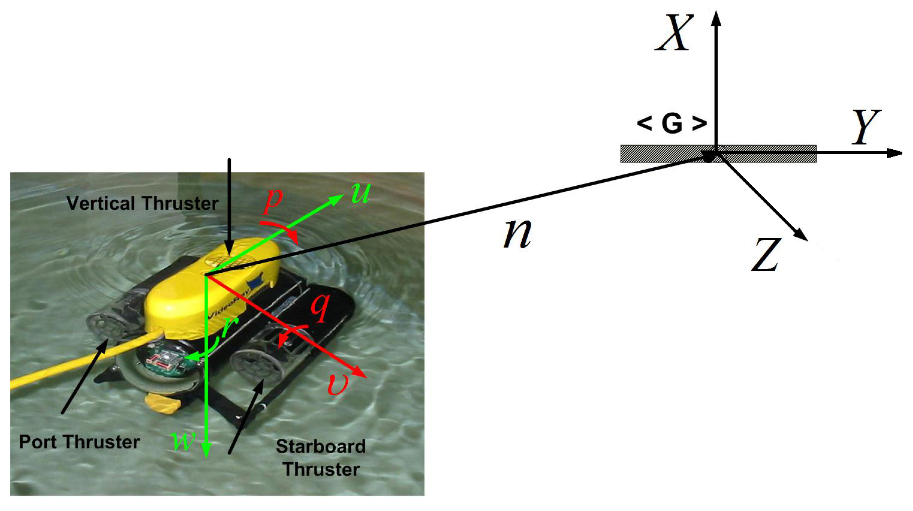
2.1. Mathematical Modeling

An autonomous underwater vehicle can be defined as a 6 Degree Of Freedom (DOF) free body with position and Euler angle vector x = [ χ y z ϕ θ ψ ] . Moreover, v = [ u υ w p q r ] is the vector of vehicle body velocities, where its components, according to SNAME [67], are surge, sway, heave, roll, pitch, and yaw, respectively (Figure 3). In addition, τ = [ X Y Z K M N ] is the vector of forces and moments acting on the vehicle center of mass. In this spirit, the dynamics of an underwater robotic vehicle are given in as [68]:
M v ˙ + C ( v ) v + D ( v ) v + g ( x ) = τ x ˙ = J ( x ) v
where: M = M RB + M A is the inertia matrix for rigid body and added mass, respectively, C ( v ) = C RB ( v ) + C A ( v ) is the Coriolis and centripetal matrix for rigid body and added mass respectively, D ( v ) = D quad ( v ) + D lin ( v ) is the quadratic and linear drag matrix, respectively, g ( x ) is the hydrostatic restoring force vector, τ , is the thruster input vector and J ( x ) is the well-known Jacobian matrix [68]. The underwater robot considered in this paper is a 3 DOF VideoRay Pro ROV (Remotely Operated underwater Vehicle) that is equipped with three thrusters, which enable it effective in surge, heave, and yaw motion (Figure 3). This means that the considered underwater robot is under-actuated along its sway axis. Here, due to the robot design, we simply neglect the angles ϕ , θ and angular velocities p and q. In addition, because of the robot symmetry regarding x-z and y-z planes we can safely assume that motions in heave, roll, and pitch are decoupled [68]. Furthermore, the coupling effects are safely can be considered to be negligible since the robot is operating at relatively low speeds. Finally, based on the aforementioned considerations, in this work we consider the kinematic model of the robot, which can be given, as follows [69]:
x k + 1 = f ( x k , V k ) + g ( x k , v k ) χ k + 1 y k + 1 z k + 1 ψ k + 1 = χ k y k z k ψ k + cos ψ k 0 0 sin ψ k 0 0 0 1 0 0 0 1 u k w k r k d t + sin ψ k cos ψ k 0 0 v k d t ,
where x k = [ χ k , y k , z k , ψ k ] is the state vector at the time-step k, including the position and orientation of the robot relative to the target frame G . Moreover, the vector of control input is V k = [ u k , w k , r k ] and d t denotes the sampling period. In addition, following theresults given in [70] and, by employing Input-to-State Stability (ISS), it can be shown that, by applying any bounded control input [ u k , r k ] to the considered nonholonomic robotic system, the velocity about the sway direction v k can be seen as a bounded disturbance with upper bound | | v k | | v ¯ that vanishes at the point x = 0 . Therefore, the aforementioned point is an equilibrium of the kinematic system of Equation (2). Note, in this work, we denote the upper bound for each variable by the notation ( · ¯ ) . Therefore, based on the aforementioned discussion, we consider the system:
x k + 1 = f ( x k , V k ) χ k + 1 y k + 1 z k + 1 ψ k + 1 = χ k y k z k ψ k + cos ψ k 0 0 sin ψ k 0 0 0 1 0 0 0 1 u k w k r k d t
as the nominal kinematic system of the underwater robotic vehicle. It is worth mentioning that the function g ( x k , v k ) Γ R 4 is considered as a bounded inner disturbance of the system that vanishes at the origin and Γ is a compact set, such that:
| | g ( x k , v k ) | | γ ¯ with γ ¯ v ¯ d t
The underwater robot that is considered in this work moves under the influence of an irrotational current, which behaves as an external disturbance to the system. The current has components with respect to the χ , y and z axes, denoted by δ χ , δ y and δ z , respectively. Moreover, we denote by δ c the slowly-varying velocity of the current that is bounded by | | δ c k | | δ ¯ c and it has direction β in χ y plane and α with respect to the z axis of the global frame, see Figure 4. In particular, we define δ k = [ δ ( χ / k ) , δ ( y / k ) , δ ( z / k ) , 0 ] Δ R 4 , with Δ being a compact set, where:
δ ( χ / k ) δ c k cos β k sin α k d t δ ( y / k ) δ c k sin β k sin α k d t δ ( z / k ) δ c k cos α k d t
It is straightforward to show that | | δ k | | δ ¯ , with δ ¯ = δ ¯ c d t . When considering the aforementioned external disturbances, the perturbed model of the underwater robotic system can be given, as follows:
x k + 1 = f ( x k , V k ) + ω k
with ω k = g ( x k , v k ) + δ k Ω R 4 as the result of adding the inner and external disturbances of the system. Ω is a compact set, such that Ω = Δ Γ , where “⊕” denotes the Minkowski addition of sets Δ and Γ . It is worth mentioning that the Minkowski addition set C of two sets A , B R n is given as C = A B = { a + b | a A , b B } . In this respect, since the sets Δ and Γ are compact, we can conclude that Ω is also a bounded compact set, which is: | | ω k | | ω ¯ with ω ¯ δ ¯ + γ ¯ .
The underwater robot is equipped by a pinhole camera with limited angles of view a and b for χ y and χ z plane, respectively. In this respect, the state vector of the system x with respect to the visual target is estimated by employing a proper vision algorithm, see Figure 4.
The requirements for the vision system, namely the visibility constraints, are imposed in order to ensure that the target will remains always within the image-plane during the control operation. That is: [ y T , y T ] [ f χ y / 1 , f χ y / 2 ] and [ z T , z T ] [ f χ z / 1 , f χ z / 2 ] , where 2 y T and 2 z T denote the width and height of the visual target. In this context, the [ f χ y / 1 , f χ y / 2 ] and [ f χ z / 1 , f χ z / 2 ] indicate the camera’s field-of-view on χ y and χ z plane, respectively (Figure 4). Moreover, we consider a maximum distance R m a x , where the visual target is visible and recognizable for the vision system. The aforementioned requirements are captured by the state constraint set X of the system, given by:
x k X R 4 ,
which is formed by:   
y + χ tan ( ψ a 2 ) y T 0
y χ tan ( ψ + a 2 ) y T 0
z χ tan ( b 2 ) z T 0
R max 2 χ 2 y 2 0
In addition, the control constraint set V s e t of the system is formulated, as follows:
V k [ u k , w k , r k ] V s e t R 3
It is worth mentioning that the control input constraints are of the form | u | u ¯ , | w | w ¯ and | r | r ¯ . Thus, we obtain V k V ¯ with V ¯ = ( u ¯ 2 + w ¯ 2 + r ¯ 2 ) 1 2 and V ¯ , u ¯ , w ¯ , r ¯ R 0 . Therefore, it can be easily shown that system Equation (3) is Lipschitz continuous:
Lemma 1.
The nominal model Equation (3), subject to constraints Equations (8b)–(8e) and (9), is locally Lipschitz in x for all x X , with a Lipschitz constant L f ( max { 8 , 8 ( u ¯ d t ) 2 } + 1 ) 1 2 .
See Appendix A.1 for the proof.

2.2. Control Design and Objective

The objective here is to guide the perturbed system Equation (6) to a desired compact set that includes the desired state x d [ χ d , y d , z d , ψ d ] X , while respecting the state and control constraints described in Equations (8b)–(8e) and (9), respectively. We employ a predictive controller in order to achieve the aforementioned objective. More specifically, the N-MPC consists in solving an Optimal Control Problem (OCP) at time instant k, with respect to a control sequence V f ( k ) [ V ( k | k ) , V ( k + 1 | k ) , , V ( k + N 1 | k ) ] , for a prediction horizon N. The OCP of the N-MPC is formulated, as follows:
min V f ( k ) J N ( x k , V f ( k ) ) =
        min V f ( k ) j = 0 N 1 F ( x ^ ( k + j | k ) , V ( k + j | k ) ) + E ( x ^ ( k + N | k ) ) subject to :
x ^ ( k + j | k ) X j , j = 1 , , N 1 ,
V ( k + j | k ) V s e t , j = 0 , , N 1 ,
x ^ ( k + N | k ) E f
where F, E, and E f are the running, terminal cost, and terminal set, respectively. The solution of the aforementioned OCP Equations (10a)–(10d) at time instant k is an optimal control sequence, being indicated as V f * ( · ) . It should be pointed out that the specifics for the design parameters, such as the running and terminal costs, as well as the state sets, will be provided in more detail in the sequel. In this context, we denote the predicted state of the nominal system Equation (3) at sampling time k + j by x ^ ( k + j | k ) , where j Z 0 . The state prediction is based on the measurement of the real system at sampling time k, denoted by x k , while applying a sequence of control inputs [ V ( k | k ) , V ( k + 1 | k ) , , V ( k + j 1 | k ) ] . Thus:
x ^ ( k + j | k ) = f ( x ^ ( k + j 1 | k ) , V ( k + j 1 | k ) )
Therefore, we have that x ^ ( k | k ) = x k . It is worth mentioning that the OCP is formulated and solved for the nominal system and for a specific time horizon. That makes it impossible to address the disturbances beforehand. However, we distinguish the nominal system, denoted as x ^ ( · ) , with the actual one denoted as x ( · ) . Therefore, we can obtain the following preliminary result:
Lemma 2.
The difference between the actual state x k + j at the time-step k + j and the predicted state x ^ ( k + j | k ) at the same time-step, under the same control sequence, is upper bounded by:
| | x k + j x ^ ( k + j | k ) | | i = 0 j 1 ( L f ) i w ¯
See Appendix A.2 for the proof.
More specifically, Lemma 2, gives the difference between the real state of the system Equation (6) with the predicted state of the nominal system Equation (3). In order to address this, we employ constraint tightening technique and use a restricted constraint set X j X in Equation (10b) instead of the state constraint set X (More details regarding the constraint tightening technique can be found in the literature [71,72]). By employing the aforementioned constraint tightening technique, we guarantee that the evolution of the perturbed system Equation (6), when the control sequence developed in Equations (10a)–(10d) is applied to it, will necessarily satisfy the state constraint set X. In particular, we denote the restricted constraint set as X j = X B j , where B j = { x R 4 : | | x | | i = 0 j 1 ( L f ) i w ¯ } . The set operator “∼” denotes the Pontryagin difference A , B R n that is defined as the set C = A B = { ζ R n : ζ + ξ A , ξ B } . Moreover, we define the running and terminal cost functions F ( · ) , E ( · ) , both of quadratic form, i.e., F ( x ^ , V ) = x ^ Q x ^ + V R V and E ( x ^ ) = x ^ P x ^ , respectively, with P, Q and R are positive definite matrices. In particular, we define Q = d i a g { q 1 , q 2 , q 3 , q 4 } , R = d i a g { r 1 , r 2 , r 3 } , and P = d i a g { p 1 , p 2 , p 3 , p 4 } . For the running cost function F, we have F ( 0 , 0 ) = 0 , and we can also obtain the following:
Lemma 3.
Regarding the cost function F ( x , V ) we have:
F ( x , V ) m i n ( q 1 , q 2 , q 3 , q 4 , r 1 , r 2 , r 3 ) | | x | | 2
See Appendix A.3 for the proof.
As we have already mentioned, the state and input constraint sets are bounded; therefore, we have:
Lemma 4.
The cost function F ( x , V ) is Lipschitz continuous in X × V s e t , with a Lipschitz constant:
L F = 2 ( R m a x 2 + z m a x 2 + ( π 2 ) 2 ) 1 2 σ m a x ( Q )
where σ m a x ( Q ) denotes the largest singular value of the matrix Q. Moreover, z m a x = R m a x tan ( b 2 ) z T is the maximum feasible value along the z axis.
See Appendix A.4 for the proof.
Before proceeding with the analysis, we employ some standard stability conditions that are used in N-MPC frameworks:
Assumption 1.
For the nominal system Equation (3), there is an admissible positively invariant set E X , such that the terminal region E f E , where E = { x X : | | x | | ε 0 } and ε 0 being a positive parameter.
Assumption 2.
We assume that in the terminal set E f , there exists a local stabilizing controller V k = h ( x k ) V s e t for all x E , and that E satisfies E ( f ( x k , h ( x k ) ) ) E ( x k ) + F ( x k , h ( x k ) ) 0 for all x E .
Assumption 3.
The terminal cost function E is Lipschitz in E , with Lipschitz constant L E = 2 ε 0 σ m a x ( P ) for all x E .
Assumption 4.
Inside the set E we have E ( x ) = x T P x α ε , where α ε = m a x { p 1 , p 2 , p 3 , p 4 } ε 0 2 > 0 . Assuming that E = { x X ( N 1 ) : h ( x ) V s e t } and taking a positive parameter α ε f , such that α ε f ( 0 , α ε ) , we assume that the terminal set designed as E f = { x R 4 : E ( x ) α ε f } is such that x E , f ( x , h ( x ) ) E f .

2.3. Problem Statement

At time step k, the solution of the N-MPC Equations (10a)–(10d) provides an control sequence, denoted as V f * ( · ) , which equals to V f * ( k ) [ V * ( k | k ) , , V * ( k + N 1 | k ) ] . In a conventional N-MPC framework, only the first control vector, i.e., V * ( k | k ) , is applied to the robotic system and the remaining parts of the optimal control sequence V f * ( k ) is discarded. At the next sampling time k + 1 , again, a new state measurement is obtained from the vision algorithm and a new OCP based on this new state measurement is calculated. This is iteratively repeated until the robot has reached to the desired position. However, the proposed self-triggered strategy in this work suggests that a portion of the computed control sequence V f * ( k ) might be applied to the underwater robot and not only the first vector. Let us suppose k i to be a triggering instant. In the proposed self-triggered control strategy, the control input that is applied to the robotic system is of the form:
[ V * ( k i | k i ) , V * ( k i + 1 | k i ) , V * ( k i + d i | k i ) ]
for all d i [ 0 , k i + 1 k i ] Z 0 , where k i + 1 is the next triggering instant. Between two consecutive triggering instants, i.e., [ k i , k i + 1 ) , the control inputs calculated by the N-MPC at the previous triggering time instant are applied to the underwater robot in an open-loop mode i.e., the vision algorithm is not activated and no image processing is performed. Obviously, the smallest and largest possible time intervals are 1 (i.e., k i + 1 = k i + 1 ) and N 1 , respectively. The self-triggered framework that is proposed in this work will provide sufficient conditions for the activation of the vision algorithm and triggering the computation of the N-MPC. Currently, we are ready to state the problem treated in this paper:
Problem 1.
Consider the system Equation (6) that is subject to the constraints Equations (7) and (9). The control goal is ( i )  to design a robust position based visual servoing control framework provided by Equations (10a)–(10d), such that the system Equation (6) converges to the desired terminal set and ( i i ) to construct a mechanism that determines when the control updates, state measurement and next VTA should occur.

3. Stability Analysis of Self-Triggering NMPC Framework

The stability analysis for the system Equations (6)–(14) is addressed in this section. It is already shown in the literature that the closed-loop system in the case of classic N-MPC is Input-to-State Stable (ISS) with respect to the disturbances [71] (More details on the notion of ISS in the discrete-time case can be found in [73].). In the subsequent analysis, we are going to use the ISS notion in order to derive the self-triggering mechanism.
The traditional approach in establishing stability in predictive control consists of two parts, named feasibility and convergence analysis. The aim in the first is to prove that the initial feasibility implies feasibility afterwards and, based on this, in the second part, it is then shown that the system state converges to a bounded set around the desired state.

3.1. Feasibility Analysis

We begin by treating the feasibility property. Before proceeding with the analysis, we provide a necessary definition:
Definition 1.
X M P C = { x 0 R n | a control sequence V f V s e t , x ^ f ( j ) X j j { 1 , , N } and x ^ ( N ) E f } .
In other words, X M P C , a set that contain all of the state vectors for which a feasible control sequence exists satisfying the constraints of the optimal control problem. Assume, now, that, at k i k , an event is triggered, thus an OCP is solved and a new control sequence V f * ( k ) [ V * ( k | k ) , , V * ( k + N 1 | k ) ] is provided. Now, consider control inputs at time instants k + m with m = 1 , , N 1 , which are based on the solution at sampling time k, V f * ( k ) . These can be defined, as follows:
V ˜ ( k + j | k + m ) = V * ( k + j | k ) for j = m , , N 1 h ( x ^ ( k + j | k + m ) ) for j = N , , N + m 1
Let N 1 control sequences V ˜ f m ( k ) be comprised by the control inputs of Equation (15), i.e.,
V ˜ f 1 ( k ) = [ V * ( k + 1 | k ) , V * ( k + 2 | k ) , , h ( x ^ ( k + N | k + 1 ) ) ] V ˜ f 2 ( k ) = [ V * ( k + 2 | k ) , , h ( x ^ ( k + N | k + 2 ) ) , h ( x ^ ( k + N + 1 | k + 2 ) ) ] V ˜ f N 1 ( k ) = [ V * ( k + N 1 | k ) ) , , h ( x ^ ( k + 2 N 2 | k + N 1 ) ) ]
Notice that the time-steps k + m are the discrete-time instants after the time-step of the triggering instant k i , i.e., [ k , k + 1 , k + 2 , , k + N 1 ] [ k i , k i + 1 , k i + 2 , , k i + N 1 ] . With the help of Assumption 2 and by taking the feasibility of the initial control sequence at sampling time k into account, it follows that, for m = 1 , N 1 , we have V ˜ ( k + j | k + m ) V s e t . We can prove finally that x ^ ( k + N + 1 | k + m ) E f for all m = 1 , , N 1 :
Proof. 
From Lemma 2, we can derive that:
| | x ^ ( k + N | k + 1 ) x ^ ( k + N | k ) | | L f N 1 w ¯ | | x ^ ( k + N | k + 2 ) x ^ ( k + N | k ) | | L f N 2 ( ( 1 + L f ) w ¯ ) | | x ^ ( k + N | k + m ) x ^ ( k + N | k ) | | L f ( N m ) i = 0 m 1 ( L f ) i w ¯
by employing the Lipschitz property of E ( · ) , we have:
E ( x ^ ( k + N | k + m ) ) E ( x ^ ( k + N | k ) ) L E | | x ^ ( k + N | k + m ) x ^ ( k + N | k ) | | L E L f ( N m ) · i = 0 m 1 ( L f ) i w ¯
Having in mind that x ^ ( k + N | k ) E f and by employing Assumption 4, we obtain the following:
E ( x ^ ( k + N | k + m ) α ε f + L E G ( m ) w ¯
with G ( m ) L f ( N m ) · i = 0 m 1 ( L f ) i . It should hold that E ( x ^ ( k + N | k + m ) ) α ε , i.e., x ^ ( k + N | k + m ) E , thus:
α ε f + L E G ( m ) w ¯ α ε w ¯ ( α ε α ε f ) L E L f ( N m ) · i = 0 m 1 ( L f ) i
Now, applying a local control law, we get x ^ ( k + N + 1 | k + m ) E f for all m = 1 , , N 1 . From these results, it can be concluded that X M P C is a robust positive invariant set if the uncertainties are bounded by Equation (16) for all m = 1 , , N 1 . Notice that Equation (16) should still hold for m = 1 for the problem to be meaningful, in the sense that it should be feasible at least in the time-triggered case. □

3.2. Convergence Analysis

Herein, we show that the state of the actual system convergences to a desired terminal set. In order to prove this, we show that a proper value function is decreasing. First, we define the optimal cost at the time-step k as J N * ( k ) = J N ( x k , V f * ( k ) ) , which is evaluated under the optimal control sequence. In the same spirit, the optimal cost at a time-step k + m with m [ 1 , N 1 ] is denoted as J N * ( k + m ) = J * ( x k + m , V f * ( k + m ) ) . Now, we denote by J ˜ N ( k + m ) the “feasible” cost, which is evaluated from the control sequence V ˜ f m ( k ) , which is J ˜ N ( k + m ) = J ˜ N ( x k + m , V ˜ f m ( k ) ) . In the following, we will employ this “feasible” cost in order to obtain the difference J N * ( k + m ) J N * ( k ) . More specifically, the difference between the optimal cost at time k and the feasible sequence at time-step k + j by employing Equation (15) is:
Δ J m = J ˜ N ( k + m ) J N * ( k ) ( L E ( L f ) ( N m ) + L F i = 0 N ( m + 1 ) ( L f ) i ) w ¯ i = 0 m 1 m i n ( q 1 , q 2 , q 3 , q 4 , r 1 , r 2 , r 3 ) | | x ^ ( k + i | k ) | |
See Appendix B for the proof. From the optimality of the solution, we have:
J N * ( k + m ) J N * ( k ) J ˜ N ( k + m ) J N * ( k )
This result along with the triggering condition that is going to be derived in the next subsection will enable us to provide conclusions for the stability and convergence of the closed-loop system.

3.3. The Self-Triggered Mechanism

This section presents the self-triggering framework that is proposed in this work. Let us consider that, at time-step k i , an event is triggered. We assume that the next triggering time k i + 1 is unknown and should be found. More specifically, triggering time k i + 1 k i + d i should be such that the closed-loop maintains its predefined desired properties. Therefore, a value function J N * ( · ) is required to be decreasing. In particular, given Equations (17) and (18), for a triggering instant k i and a number of time-step d i after k i , with d i = 1 , 2 , , N 1 it can be obtained the following:
J N * ( k i + 1 ) J N * ( k i ) ( L E ( L f ) ( N d i ) + L F i = 0 N ( d i + 1 ) ( L f ) i ) w ¯ L Q ( d i )
where:
L Q ( d i ) = i = 0 d i 1 m i n ( q 1 , q 2 , q 3 , q 4 , r 1 , r 2 , r 3 ) | | x ^ ( k + i | k ) | |
The time instant k i + 1 should be such that:   
( L E ( L f ) ( N d i ) + L F i = 0 i = N ( d i + 1 ) ( L f ) i ) w ¯ σ L Q ( d i ) ,
where 0 < σ < 1 . Substituting Equation (20) to (19), we obtain
J N * ( k i + 1 ) J N * ( k i ) ( σ 1 ) L Q ( d i )
This suggests that, by considering 0 < σ < 1 , decreasing of the value function is guaranteed. In particular, in view of Equation (21), we can conclude that the value function J N * ( · ) has been proven to be decreasing at the triggering instants. Next, we study the convergence of the state of the system under the proposed self-triggered framework:

Convergence of System under the Proposed Self-Triggered Framework

We have proven in Equation (20) that the value function J N * ( · ) is always decreasing with respect to the previous triggering instant. In other words, the value function cannot be guaranteed to be monotonically decreasing at every time-step, as the standard Lyapunov theory dictates. Thus, additional arguments will be provided in order to prove convergence of the state of the closed-loop system to a bounded set. In particular, the following steps are going to be followed: first, we are going to provide the steps to derive a suitable Lyapunov-function candidate and, secondly, we are going to show that this Lyapunov function is an ISS-Lyapunov function and, according to standard definitions, if a system admits an ISS-Lyapunov function, then the system is ISS with respect to the external disturbances, [73]. Thus, finding a suitable ISS-Lyapunov function immediately implies that our system is ISS with respect to disturbances and, thus, the states of the closed-loop system are converging to a bounded set.
Proposition 1.
Our proposed Lyapunov function candidate is the following:
W ( k ) J N * ( k ) for d i = 1 j = 1 d i 1 { J N * ( k + j ) · ( d i j ) } + d i J N * ( k ) for d i > 1
Now, if d i = 1 at every time instant then our system boils down to the classic time-triggered MPC, where, in [71], it has been shown that the closed-loop system is ISS with respect to the disturbances. However, we are going to show that Equation (22) is also an ISS-Lyapunov function for d i 1 . This is going to be shown for d 1 = 2 and then Equation (22) is derived by induction.
Proof. 
Now, assume that d i = 2 . From Equation (19), it follows that:
J N * ( k + 1 ) J N * ( k ) ( L E ( L f ) ( N 1 ) + L F i = 0 N 2 ( L f ) i ) w ¯ L Q ( 1 ) ,
as well as:
J N * ( k + 2 ) J N * ( k ) ( L E ( L f ) ( N 2 ) + L F i = 0 N 3 ( L f ) i ) w ¯ L Q ( 2 )
adding the last two inequalities, yields:
J N * ( k + 2 ) + J N * ( k + 1 ) 2 J N * ( k ) ( L Q ( 1 ) + L Q ( 2 ) ) + ( L E ( L f ) ( N 2 ) + L F i = 0 N 3 ( L f ) i ) ( 1 + L f ) w ¯
adding and subtracting the terms j = 1 d i 1 J N * ( k + j ) ( d i j ) in Equation (23), we can obtain:   
J N * ( k + 2 ) + 2 J N * ( k + 1 ) J N * ( k + 1 ) + 2 J N * ( k ) + ( L E ( L f ) ( N 2 ) + L F i = 0 N 3 ( L f ) i ) ( 1 + L f ) w ¯ ( L Q ( 1 ) + L Q ( 2 ) )
Considering as a Lyapunov function:
W ( k ) = J N * ( k + 1 ) + 2 J N * ( k )
Equation (24) is re-written as:
W ( k + 1 ) W ( k ) + ( L E ( L f ) ( N 2 ) + L F i = 0 N 3 ( L f ) i ) ( 1 + L f ) w ¯ ( L Q ( 1 ) + L Q ( 2 ) )
It is now evident that, by induction, we can reach to Equation (22) for an arbitrary d i , following the same procedure. Moreover, from Equation (25), it is obvious that W ( k ) , as defined in Equation (22), is an ISS-Lyapunov function, thus the proposed framework is ISS stable with respect to the external disturbances and the proof is completed. □
Thus, having the aforementioned analysis in mind, the next tracking of the vision system as well as updating the control law should be occur when Equation (20) is violated. This means that, at the triggering time instance, the condition Equation (20) must be checked for each consecutive time-step, i.e., for d i = 1 , 2 , . Thus, we check which time step does not meet this condition and set it to the next triggering instant k i + 1 . Based on the above discussion, it can be understood that, in the proposed self-activated framework, the time step k i + 1 is found beforehand at time k i . Moreover, it is worth mentioning that the term L Q ( d i ) only includes predictions of the nominal system that can be easily computed by forward integration of Equation (3) for time-steps d i [ 1 , N 1 ] . Now, based on the aforementioned stability results, we state the theorem for the proposed vision-based self-triggered framework:
Theorem 1.
Consider the system of autonomous underwater vehicle described by Equation (6), which is subject to state and input constraints given in Equations (7) and (9) under the N-MPC framework and assume that the Assumptions 1–4 hold. The vision tracking and control update times that are provided by Equation (20) and the N-MPC framework given in Equations (10a)–(10d), which is applied to the autonomous underwater vehicle in an open-loop fashion during the inter-sampling periods, drive the closed-loop system into the terminal set E f that includes the desired pose configuration with respect to the visual target.
The pseudo-code description of the proposed real-time self-triggering position that is based visual servoing is given in Algorithm 1:
Algorithm 1 Real-time algorithm of the proposed self Triggered PBVS-NMPC framework:
1:
Triggering time:
▷ At triggering time k i
2:
   x ( k i ) VTA
▷ Trigger the VTA, get s ( k i )
3:
   V f * ( k i ) OCP ( x ( k i ) )
▷ Run OCP of (10a)–(10d)
4:
   k i + 1 = k i + d i Solve Equation (20) for d i
▷ The next triggering time
5:
for   i = 1 d i do
6:
  Apply the control inputs V * ( k i + i | k i ) to the underwater robot.
7:
gotoTriggering time.
At time k i , we assume that the Vision Tracking Algorithm (VTA) is triggered, the optimal control problem of the N-MPC Equations (10a)–(10d) is run and a control sequence for the time interval [ k i , k i + N 1 ] is provided. The solution of Equation (20) provides the next triggering time k i + 1 , as it is already stated. During the time interval i [ k i , k i + 1 ) , the control inputs V * ( k i + i | k i ) are applied to the underwater robot in an open-loop fashion. Next, at k i + 1 the vision system is tracked and the OCP of the N-MPC Equations (10a)–(10d) is solved again while employing the new state measurement x ( k i + 1 ) as the initial values in Equations (10a)–(10d). The controller follows this procedure until the robot converges and stabilizes towards the visual target.

4. Experiments

In this section, the efficacy of the proposed position based self triggered framework demonstrated through a real time comparative experimental study. A real-time stabilization scenario was considered by employing a small and under-actuated underwater vehicle.

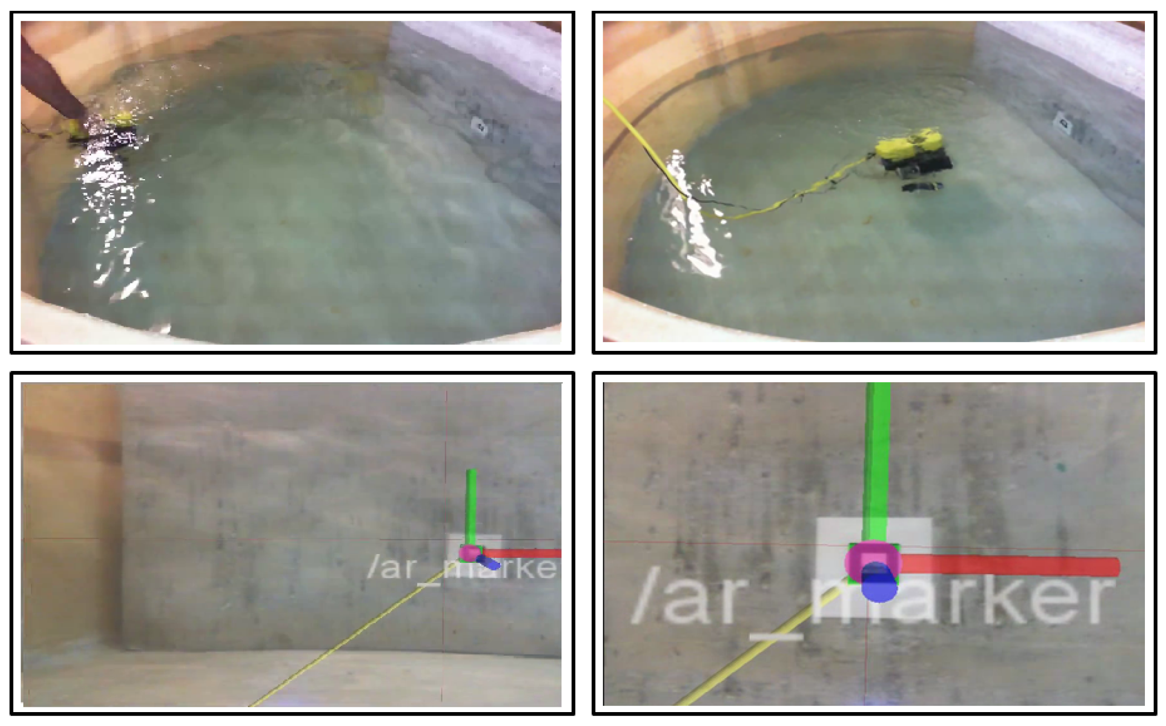
4.1. System Components

The small underwater robot used in following experiments is a 3-DOF (VideoRay PRO, VideoRay LLC, Figure 3), which is equipped with 3 thrusters, and a USB camera. The image dimensions are 640x480 pixels. A visual target is located on an aluminum surface plane that is fixed inside the tank. The system software is conducted in the Robotics Operating System (ROS, http://www.ros.org), and the code is written in C++ and Python.
The state vector of the underwater robot regarding the visual target is estimated in real time while using the ROS package ar_pose (http://www.ros.org/wiki/ar_pose), which is an Augmented Reality Marker Pose Estimation algorithm that is based on the ARToolkit software library (http://www.hitl.washington.edu/artoolkit/). The target detection and robot localization in initial and desired pose configuration are shown in Figure 5. The constrained N-MPC that was used in this real-time experiment was designed using the NLopt Optimization library [74].

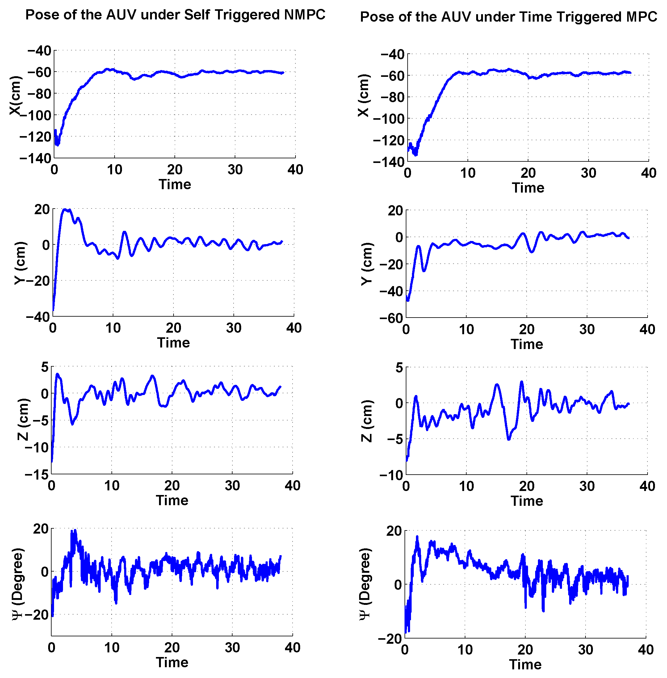
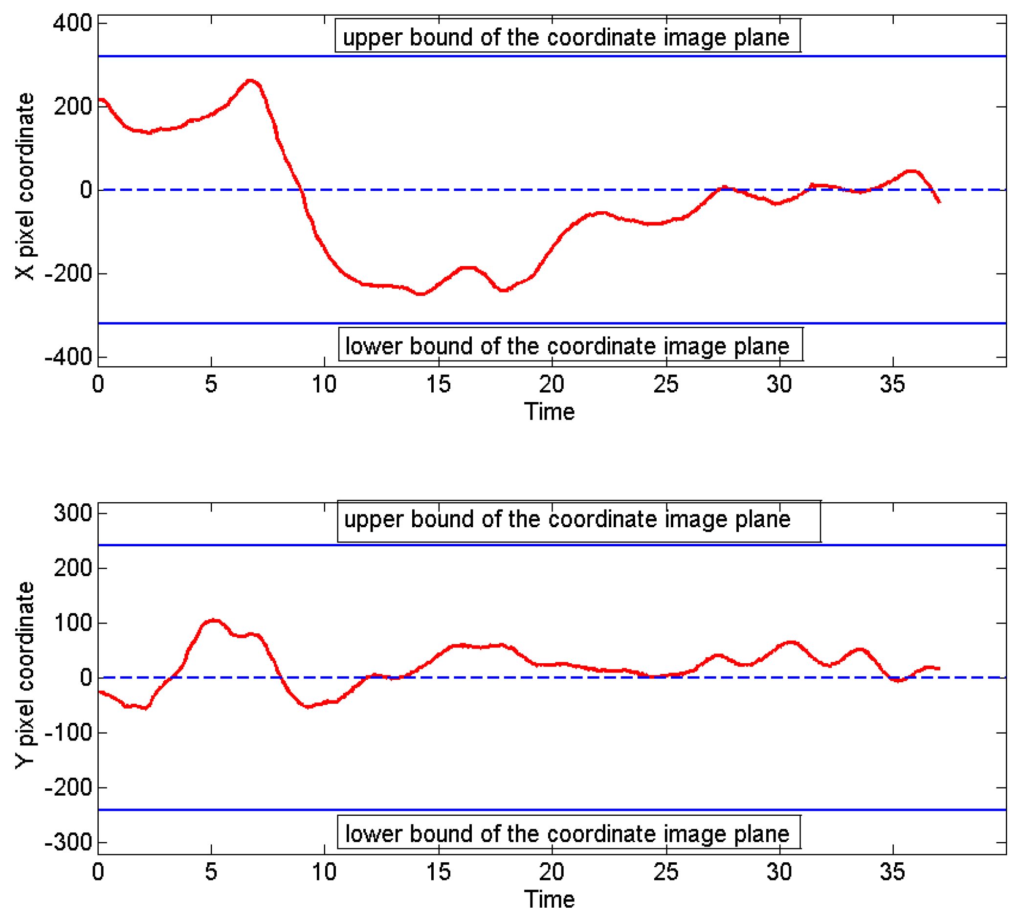
4.2. Experimental Results

The goal in the following comparative experimental studies is the stabilization of the underwater robot at the desired configuration towards the visual target. Two experiments were held for comparison. More specifically, in the first experiment, we employed a classic N-MPC (i.e., time activation at each sampling time), while, in the second experiment, the self-triggered framework proposed in this work was used. The initial as well as desired position of the underwater vehicle relative to the target frame is [ χ i n , y i n , z i n , ψ i n ] = [ 1.2 , 0.45 , 0.1 , 0.401 ] and x d = [ χ d , y d , z d , ψ d ] = [ 0.6 , 0.0 , 0.0 , 0.0 ] , respectively. In the initial pose, the target appears in the right side of the camera view because of the negative yaw angles of the vehicle with respect to the target frame (See Figure 5). Note that this is a difficult initial pose and, if one does not take the visual constraints into account, the experiment will fail. The sampling time and prediction horizon were selected as to be d t = 0.15 sec and N = 6 , respectively. It is worth mentioning that the sampling time is selected based on the response frequency of the closed-loop system, while the prediction horizon is selected based on the computational capabilities of the onboard unit to solve the optimization problem. The more capable the computational unit is, the larger the prediction horizon can be considered. The maximum allowable velocities for the considered underwater robot in surge, heave, and yaw direction were selected as u ¯ = 0.2 m/s, w ¯ = 0.3 m/s and r ¯ = 0.3 rad/s, respectively. It is worth mentioning that the considered allowable velocities might be required for the needs of several common underwater tasks (e.g., seabed inspection, mosaicking), where the vehicle is required to move with relatively low speeds with a predefined upper bound. The design matrices Q, R, and P are defined as Q = d i a g ( 0.5 , 4.5 , 4.5 , 0.1 ) , R = d i a g ( 0.17 , 0.1 , 1 ) , and P = d i a g ( 1 , 1 , 1 , 1 ) , respectively. The maximum permissible distance on the referred water tank is R m a x = 1.5 m. The results of the experiment are presented in Figure 6, Figure 7, Figure 8, Figure 9 and Figure 10. In Figure 6, the evolution of the robot coordinates in x, y, and ψ for both experiments are depicted. When comparing two experiments, it is obvious that the underwater robot in both experiments has reached and stabilized in the desired position towards the visual target and the operational limitations (F.O.V and control saturation) remained satisfied. It can also be seen that the system performances in the case of proposed self triggering framework are better (or at least the same) as compared to the classical approach.
In Figure 7 and Figure 8, the camera view and the coordinates of the visual target center during the experiments are presented, respectively. It is obvious that the target remains inside of the F.O.V of the camera. Figure 9 presents the triggering evaluation in the case of the proposed self triggered framework. For the value 1 in vertical axis, the vision algorithm has been activated, thus the image has been processed, the state vector has been estimated, N-MPC has been evaluated, and control inputs are calculated. For value 0, the rest of the last computed control inputs implemented on the underwater robot in an open-loop fashion, and, therefore, no optimization and no image processing is running. Moreover, in the case of classic N-MPC, vision tracking and N-MMPC are running always at all sampling times, as has been already stated. It is worth mentioning that by employing the proposed self triggered condition, the triggering of the vision tracking algorithm and the N-MPC have been reduced by 50% (124 triggering instead of 253) regarding the classic N-MPC framework. When comparing the triggering instants of Figure 9 to the image target center coordinate in Figure 8, one might notice that when the target is going to leave the image plane (at the region of six and 14–17 s of the experiment), the triggering instants are more frequent. This fact appears at region of the 40 and the 80–110 sampling times, respectively, in the Figure 9. When comparing triggering instants of Figure 9 to the state evolution of the system Figure 6, one might notice that when the robot is getting near to the desired position the triggering instants are more frequent. This is because, close to the desired position, the system becomes more demanding due to the visibility limitations as the target becomes larger in the camera view and because external disturbances move the robot from the desired position.
The computational time in the case when a new state information from vision system and a new control sequence are calculated (triggering instant) is approximately 0.1 s, while, in the case of the open loop control (employing the proposed self triggered framework), it is being reduced to 0.0002 s. This is because, in the case of self-triggering framework, neither the vision tracking algorithm nor the optimization process is executed between two triggering instants. Finally, Figure 10 presents the control inputs during the experiments. It is easy to see that the control constraints remained satisfied during the experiment.

4.3. Video

This work is accompanied by a video presenting the experimental procedure of Section 4: https://youtu.be/mdRM2ThaOQM.

5. Conclusions

In this paper, a self-triggered position-based visual servoing control framework for autonomous underwater vehicles was presented. The main idea of this work is to activate the vision tracking algorithm and the optimization of the N-MPC in an aperiodic way, which is only when required and not in each sampling time. By employing the proposed vision-based self-triggered control strategy, both the control inputs and the next activation time are evaluated to avoid continuous measurements from the vision system. During the inter-sampling instants, the control inputs that are calculated by N-MPC are applied to the underwater robot in an open-loop mode and, therefore, no optimization and no image processing is running between two triggering instants. This results in a reduction in processing time as well as energy consumption and, therefore, increases the accuracy and autonomy of the Autonomous Underwater Vehicle. The latter is of paramount importance for persistent underwater inspection tasks. Rigorous robustness analysis, along with sufficient conditions for triggering, is provided in this work. The effectiveness of the proposed vision-based self-triggered control framework is verified through a comparative experimental study using an underwater robot. In these experiments, by employing the proposed self triggered control strategy, we achieved a significant 50% reduction in the activation of the vision tracking algorithm and the OCP as compared to the classic N-MPC framework. Future research efforts will be devoted towards extending the proposed methodology for multiple Autonomous Underwater Vehicles, including not only static, but also moving target as well as conducting complex real-time experiments employing a team of cooperative AUVs.

Author Contributions

Conceptualization, S.H.-a.; methodology, S.H.-a., A.E., D.V.D.; software, S.H.-a., G.C.K.; validation, S.H.-a., G.K. and A.E.; investigation, S.H.-a., G.C.K.; writing–original draft preparation, S.H.-a., A.E., G.C.K.; writing–review and editing, S.H.-a.; supervision, K.J.K.; project administration, S.H.-a., K.J.K. All authors have read and agreed to the published version of the manuscript.

Funding

This work was supported by the EU funded project PANDORA: Persistent Autonomy through learNing, aDaptation, Observation and ReplAnning, F P 7288273 , 20122014.

Conflicts of Interest

The authors declare no conflict of interest.

Appendix A.

Appendix A.1. The Proof of Lemma 1:

The Euclidean norm is used for the sake of simplicity. We get:
| | f ( x 1 , V ) f ( x 2 , V ) | | 2 = | | χ 1 + cos ψ 1 u d t χ 2 cos ψ 2 u d t y 1 + sin ψ 1 u d t y 2 sin ψ 2 u d t z 1 z 2 ψ 1 ψ 2 | | 2 = | χ 1 χ 2 + u d t ( cos ψ 1 cos ψ 2 ) | 2 + | z 1 z 2 | 2 + | ψ 1 ψ 2 | 2 + | y 1 y 2 + u d t ( sin ψ 1 sin ψ 2 ) | 2
From the mean value theorem, we can obtain:
| | cos ψ 1 cos ψ 2 | | = | | sin ψ * ( ψ 1 ψ 2 ) | | | | ψ 1 ψ 2 | |
where ψ * ( ψ 1 , ψ 2 ) . This yields the following:
| χ 1 χ 2 + u d t ( cos ψ 1 cos ψ 2 ) | 2 [ 2 max { | χ 1 χ 2 | , u d t | cos ψ 1 cos ψ 2 | } ] 2 4 max { ( χ 1 χ 2 ) 2 , ( u d t ) 2 ( ψ 1 ψ 2 ) 2 } max { 4 , 4 ( u d t ) 2 } max { ( χ 1 χ 2 ) 2 , ( ψ 1 ψ 2 ) 2 } max { 4 , 4 ( u ¯ d t ) 2 } [ ( χ 1 χ 2 ) 2 + ( ψ 1 ψ 2 ) 2 ]
Applying similar derivations to the other elements, it can be concluded that for all x 1 , x 2 X it can be obtained:
| | f ( x 1 , V ) f ( x 2 , V ) | | 2 max { 4 , 4 ( u ¯ d t ) 2 } [ ( χ 1 χ 2 ) 2 + ( ψ 1 ψ 2 ) 2 ] + ( z 1 z 2 ) 2 + max { 4 , 4 ( u ¯ d t ) 2 } [ ( y 1 y 2 ) 2 + ( ψ 1 ψ 2 ) 2 ] + ( ψ 1 ψ 2 ) 2 = max { 4 , 4 ( u ¯ d t ) 2 } [ ( χ 1 χ 2 ) 2 + ( y 1 y 2 ) 2 + 2 ( ψ 1 ψ 2 ) 2 ] + ( z 1 z 2 ) 2 + ( ψ 1 ψ 2 ) 2 ( max { 8 , 8 ( u ¯ d t ) 2 } + 1 ) [ ( χ 1 χ 2 ) 2 + ( y 1 y 2 ) 2 + ( ψ 1 ψ 2 ) 2 + ( z 1 z 2 ) 2 ] ( max { 8 , 8 ( u ¯ d t ) 2 } + 1 ) | | x 1 x 2 | | 2
thus the Lipschitz constant is L f ( max { 8 , 8 ( u ¯ d t ) 2 } + 1 ) 1 / 2 , with 0 < L f < and that concludes the proof.

Appendix A.2. The Proof of Lemma 2:

Using Lemma 1 and the triangle inequality we get:
| | x k + 1 x ^ ( k + 1 | k ) | | = | | f ( x k , V k ) + w k f ( x ^ ( k | k ) , V k ) | | = | | w k | | w ¯ | | x k + 2 x ^ ( k + 2 | k ) | | = | | f ( x k + 1 , V k + 1 ) + w k + 1 f ( x ^ ( k + 1 | k ) , V k + 1 ) | | | | f ( x k + 1 , V k + 1 ) f ( x ^ ( k + 1 | k ) , V k + 1 ) | | + | | w k + 1 | | L f | | x k + 1 x ^ ( k + 1 | k ) | | + | | w k + 1 | | ( 1 + L f ) w ¯ | | x k + j x ^ ( k + j | k ) | | i = 0 j 1 ( L f ) i w ¯

Appendix A.3. The Proof of Lemma 3:

F ( x , V ) = x d i a g ( q 1 , q 2 , q 3 ) x + V d i a g ( r 1 , r 2 ) V = [ x , V ] d i a g ( q 1 , q 2 , q 3 , r 1 , r 2 ) [ x , V ] m i n ( q 1 , q 2 , q 3 , r 1 , r 2 ) | | [ x , V ] | | 2 min ( q 1 , q 2 , q 3 , r 1 , r 2 ) | | x | | 2

Appendix A.4. The Proof of Lemma 4:

| | F ( x 1 , V ) F ( x 2 , V ) | | = | | x 1 Q x 1 x 2 Q x 2 | | = | | x 1 Q x 1 x 1 Q x 2 + x 1 Q x 2 x 2 Q x 2 | | = | | x 1 Q ( x 1 x 2 ) + + ( x 1 x 2 ) Q x 2 | | = | | x 1 Q ( x 1 x 2 ) + x 2 Q ( x 1 x 2 ) | | = | | ( x 1 + x 2 ) Q ( x 1 x 2 ) | | ( | | x 1 | | + | | x 2 | | ) σ m a x ( Q ) | | x 1 x 2 | |
Notice that x X we have: | | x | | = ( | χ | 2 + | y | 2 + | z | 2 + | ψ | 2 ) 1 2 ( R m a x 2 + z m a x 2 + ( π 2 ) 2 ) 1 2 , which concludes the proof. Notice that the maximum value z m a x along the z-axis is calculated by substituting the maximum feasible distance R m a x into the visibility constraints of Equation (8c).

Appendix B. Lyapunov Function

Δ J m = J ˜ N ( k + m ) J N * ( k ) = i = 0 N 1 F ( x ˜ ( k + i + m | k + m ) , V ˜ ( k + i + m | k + m ) ) i = 0 N 1 F ( x ^ ( k + i | k ) , V * ( k + i | k ) ) + E ( x ˜ ( k + N + m | k + m ) ) E ( x ^ ( k + N | k ) ) = i = 0 N ( m + 1 ) { F ( x ˜ ( k + i + m | k + m ) , V ˜ ( k + i + m | k + m ) ) F ( x ^ ( k + i + m | k ) , V * ( k + i + m | k ) ) } i = 0 m 1 F ( x ^ ( k + i | k ) , V * ( k + i | k ) ) + i = 1 m F ( x ˜ ( k + N 1 + i | k + m ) , h ( x ˜ ( k + N 1 + i | k + m ) ) ) + E ( x ˜ ( k + N + m | k + m ) ) E ( x ^ ( k + N | k ) )
with x ˜ ( k + i | k + m ) denoting the “feasible” state of the system which accounts for the predicted state at time-step k + i , based on the measurement of the real state at time-step k + m , when the feasible control sequence from Equation (15) is used. Also from Lemma 2 and with the help of Lemma 4, it yields:
i = 0 N ( m + 1 ) { F ( x ˜ ( k + i + m | k + m ) , V ˜ ( k + i + m | k + m ) ) F ( x ^ ( k + i + m | k ) , V * ( k + i + m | k ) ) } L F i = 0 N ( m + 1 ) ( L f ) i w ¯
Using i = 0 m 1 E ( x ˜ ( k + N + i | k + m ) ) E ( x ˜ ( k + N + i | k + m ) ) which adds up to zero, while taking into account Assumption 2, it can be obtained:
F ( x ˜ ( k + N 1 + m | k + m ) , h ( x ˜ ( k + N 1 + m | k + m ) ) ) + E ( x ˜ ( k + N + m | k + m ) ) E ( x ˜ ( k + N 1 + m | k + m ) ) 0
Moreover:
E ( x ˜ ( k + N | k + m ) ) E ( x ^ ( k + N | k ) ) L E ( L f ) ( N m ) w ¯
Also, using Lemma (3) we get:
i = 0 m 1 F ( x ^ ( k + i | k ) , V * ( k + i | k ) ) i = 0 m 1 m i n ( q 1 , q 2 , q 3 , q 4 , r 1 , r 2 , r 3 ) | | x ^ ( k + i | k ) | |
Substituting all these inequalities to the difference Δ J m , yields:
Δ J m = J ˜ N ( k + m ) J N * ( k ) ( L E ( L f ) ( N m ) + L F i = 0 N ( m + 1 ) ( L f ) i ) w ¯ i = 0 m 1 m i n ( q 1 , q 2 , q 3 , q 4 , r 1 , r 2 , r 3 ) | | x ^ ( k + i | k ) | |

References

  1. Hu, Y.; Zhao, W.; Xie, G.; Wang, L. Development and target following of vision-based autonomous robotic fish. Robotica 2009, 27, 1075–1089. [Google Scholar] [CrossRef]
  2. Pérez-Alcocer, R.; Torres-Méndez, L.A.; Olguín-Díaz, E.; Maldonado-Ramírez, A.A. Vision-based autonomous underwater vehicle navigation in poor visibility conditions using a model-free robust control. J. Sens. 2016, 2016, 8594096. [Google Scholar] [CrossRef] [Green Version]
  3. Xiang, X.; Jouvencel, B.; Parodi, O. Coordinated formation control of multiple autonomous underwater vehicles for pipeline inspection. Int. J. Adv. Robot. Syst. 2010, 7, 75–84. [Google Scholar] [CrossRef]
  4. Allibert, G.; Hua, M.D.; Krupínski, S.; Hamel, T. Pipeline following by visual servoing for Autonomous Underwater Vehicles. Control. Eng. Pract. 2019, 82, 151–160. [Google Scholar] [CrossRef] [Green Version]
  5. Adegboye, M.A.; Fung, W.K.; Karnik, A. Recent advances in pipeline monitoring and oil leakage detection technologies: Principles and approaches. Sensors 2019, 19, 2548. [Google Scholar] [CrossRef] [Green Version]
  6. Zhang, J.; Zhang, Q.; Xiang, X. Automatic inspection of subsea optical cable by an autonomous underwater vehicle. In Proceedings of the OCEANS 2017-Aberdeen, Aberdeen, Scotland, 19–22 June 2017; pp. 1–6. [Google Scholar]
  7. Xiang, X.; Yu, C.; Niu, Z.; Zhang, Q. Subsea cable tracking by autonomous underwater vehicle with magnetic sensing guidance. Sensors 2016, 16, 1335. [Google Scholar] [CrossRef] [PubMed] [Green Version]
  8. Hansen, R.E.; Lågstad, P.; Sæbø, T.O. Search and Monitoring of Shipwreck and Munitions Dumpsites Using HUGIN AUV with Synthetic Aperture Sonar–Technology Study; FFI: Kjeller, Norway, 2019. [Google Scholar]
  9. Denniston, C.; Krogstad, T.R.; Kemna, S.; Sukhatme, G.S. On-line AUV Survey Planning for Finding Safe Vessel Paths through Hazardous Environments. In Proceedings of the 2018 IEEE/OES Autonomous Underwater Vehicle Workshop (AUV), Porto, Portugal, 6–9 November 2018; pp. 1–8. [Google Scholar]
  10. Huebner, C.S. Evaluation of side-scan sonar performance for the detection of naval mines. In Proceedings of the Target and Background Signatures IV, Berlin, Germany, 10–11 September 2018. [Google Scholar]
  11. Heshmati-Alamdari, S.; Bechlioulis, C.P.; Liarokapis, M.V.; Kyriakopoulos, K.J. Prescribed performance image based visual servoing under field of view constraints. In Proceedings of the 2014 IEEE/RSJ International Conference on Intelligent Robots and Systems, Chicago, IL, USA, 14–18 September 2014; pp. 2721–2726. [Google Scholar]
  12. Chaumette, F.; Hutchinson, S. Visual Servo Control Part I: Basic Approaches. IEEE Robot. Autom. Mag. 2006, 13, 82–90. [Google Scholar] [CrossRef]
  13. Chaumette, F.; Hutchinson, S. Visual Servo Control Part II: Advanced Approaches. IEEE Robot. Autom. Mag. 2007, 14, 109–118. [Google Scholar] [CrossRef]
  14. Bechlioulis, C.P.; Heshmati-alamdari, S.; Karras, G.C.; Kyriakopoulos, K.J. Robust image-based visual servoing with prescribed performance under field of view constraints. IEEE Trans. Robot. 2019, 35, 1063–1070. [Google Scholar] [CrossRef]
  15. Rives, P.; Borrelly, J.J. Visual servoing techniques applied to underwater vehicles. In Proceedings of the 1997 IEEE/RSJ International Conference on Intelligent Robot and Systems, Grenoble, France, 11 September 1997; Volume 3. [Google Scholar]
  16. Krupiski, S.; Allibert, G.; Hua, M.D.; Hamel, T. Pipeline tracking for fully-actuated autonomous underwater vehicle using visual servo control. In Proceedings of the American Control Conference, Montreal, QC, Canada, 27–29 June 2012; pp. 6196–6202. [Google Scholar]
  17. Karras, G.; Loizou, S.; Kyriakopoulos, K. Towards semi-autonomous operation of under-actuated underwater vehicles: Sensor fusion, on-line identification and visual servo control. Auton. Robot. 2011, 31, 67–86. [Google Scholar] [CrossRef]
  18. Silpa-Anan, C.; Brinsmead, T.; Abdallah, S.; Zelinsky, A. Preliminary experiments in visual servo control for autonomous underwater vehicle. In Proceedings of the 2001 IEEE/RSJ International Conference on Intelligent Robots and Systems, Maui, HI, USA, 29 October–3 November 2001; Volume 4, pp. 1824–1829. [Google Scholar]
  19. Negahdaripour, S.; Firoozfam, P. An ROV stereovision system for ship-hull inspection. IEEE J. Ocean. Eng. 2006, 31, 551–564. [Google Scholar] [CrossRef]
  20. Lee, P.M.; Jeon, B.H.; Kim, S.M. Visual servoing for underwater docking of an autonomous underwater vehicle with one camera. Oceans Conf. Rec. (IEEE) 2003, 2, 677–682. [Google Scholar]
  21. Park, J.Y.; Jun, B.h.; Lee, P.m.; Oh, J. Experiments on vision guided docking of an autonomous underwater vehicle using one camera. Ocean Eng. 2009, 36, 48–61. [Google Scholar] [CrossRef]
  22. Lots, J.F.; Lane, D.; Trucco, E. Application of 2 1/2 D visual servoing to underwater vehicle station-keeping. Oceans Conf. Rec. (IEEE) 2000, 2, 1257–1262. [Google Scholar]
  23. Cufi, X.; Garcia, R.; Ridao, P. An approach to vision-based station keeping for an unmanned underwater vehicle. In Proceedings of the IEEE International Conference on Intelligent Robots and Systems, Lausanne, Switzerland, 30 September–4 October 2002; Volume 1, pp. 799–804. [Google Scholar]
  24. Van der Zwaan, S.; Bernardino, A.; Santos-Victor, J. Visual station keeping for floating robots in unstructured environments. Robot. Auton. Syst. 2002, 39, 145–155. [Google Scholar] [CrossRef] [Green Version]
  25. Heshmati-Alamdari, S.; Karras, G.C.; Kyriakopoulos, K.J. A distributed predictive control approach for cooperative manipulation of multiple underwater vehicle manipulator systems. In Proceedings of the 2019 International Conference on Robotics and Automation (ICRA), Montreal, QC, Canada, 20–24 May 2019; pp. 4626–4632. [Google Scholar]
  26. Heshmati-Alamdari, S.; Bechlioulis, C.P.; Karras, G.C.; Nikou, A.; Dimarogonas, D.V.; Kyriakopoulos, K.J. A robust interaction control approach for underwater vehicle manipulator systems. Annu. Rev. Control. 2018, 46, 315–325. [Google Scholar] [CrossRef]
  27. Fossen, T. Handbook of Marine Craft Hydrodynamics and Motion Control; John Wiley & Sons: Hoboken, NJ, USA, 2011. [Google Scholar] [CrossRef]
  28. Al Makdah, A.A.R.; Daher, N.; Asmar, D.; Shammas, E. Three-dimensional trajectory tracking of a hybrid autonomous underwater vehicle in the presence of underwater current. Ocean Eng. 2019, 185, 115–132. [Google Scholar] [CrossRef]
  29. Moon, J.H.; Lee, H.J. Decentralized Observer-Based Output-Feedback Formation Control of Multiple Unmanned Underwater Vehicles. J. Electr. Eng. Technol. 2018, 13, 493–500. [Google Scholar]
  30. Zhang, J.; Yu, S.; Yan, Y. Fixed-time output feedback trajectory tracking control of marine surface vessels subject to unknown external disturbances and uncertainties. ISA Trans. 2019, 93, 145–155. [Google Scholar] [CrossRef]
  31. Paliotta, C.; Lefeber, E.; Pettersen, K.Y.; Pinto, J.; Costa, M. Trajectory tracking and path following for underactuated marine vehicles. IEEE Trans. Control. Syst. Technol. 2018, 27, 1423–1437. [Google Scholar] [CrossRef] [Green Version]
  32. Do, K.D. Global tracking control of underactuated ODINs in three-dimensional space. Int. J. Control. 2013, 86, 183–196. [Google Scholar] [CrossRef]
  33. Li, Y.; Wei, C.; Wu, Q.; Chen, P.; Jiang, Y.; Li, Y. Study of 3 dimension trajectory tracking of underactuated autonomous underwater vehicle. Ocean Eng. 2015, 105, 270–274. [Google Scholar] [CrossRef]
  34. Aguiar, A.; Pascoal, A. Dynamic positioning and way-point tracking of underactuated AUVs in the presence of ocean currents. Int. J. Control. 2007, 80, 1092–1108. [Google Scholar] [CrossRef]
  35. Heshmati-Alamdari, S.; Karras, G.C.; Marantos, P.; Kyriakopoulos, K.J. A Robust Predictive Control Approach for Underwater Robotic Vehicles. IEEE Trans. Control. Syst. Technol. 2019. [Google Scholar] [CrossRef]
  36. Bechlioulis, C.P.; Karras, G.C.; Heshmati-Alamdari, S.; Kyriakopoulos, K.J. Trajectory tracking with prescribed performance for underactuated underwater vehicles under model uncertainties and external disturbances. IEEE Trans. Control. Syst. Technol. 2016, 25, 429–440. [Google Scholar] [CrossRef]
  37. Heshmati-alamdari, S.; Nikou, A.; Dimarogonas, D.V. Robust Trajectory Tracking Control for Underactuated Autonomous Underwater Vehicles. In Proceedings of the 2019 IEEE 58th Conference on Decision and Control (CDC), Nice, France, 11–13 December 2019; pp. 8311–8316. [Google Scholar]
  38. Xiang, X.; Lapierre, L.; Jouvencel, B. Smooth transition of AUV motion control: From fully-actuated to under-actuated configuration. Robot. Auton. Syst. 2015, 67, 14–22. [Google Scholar] [CrossRef] [Green Version]
  39. Heshmati-Alamdari, S. Cooperative and Interaction Control for Underwater Robotic Vehicles. Ph.D. Thesis, National Technical University of Athens, Athens, Greece, 2018. [Google Scholar]
  40. Allgöwer, F.; Findeisen, R.; Nagy, Z. Nonlinear model predictive control: From theory to application. Chin. Inst. Chem. Eng. 2004, 35, 299–315. [Google Scholar]
  41. Allibert, G.; Courtial, E.; Chaumette, F. Predictive control for constrained image-based visual servoing. IEEE Trans. Robot. 2010, 26, 933–939. [Google Scholar] [CrossRef] [Green Version]
  42. Sauvee, M.; Poignet, P.; Dombre, E.; Courtial, E. Image based visual servoing through nonlinear nodel predictive control. In Proceedings of the IEEE Conference on Decision and Control, San Diego, CA, USA, 13–15 December 2006; pp. 1776–1781. [Google Scholar]
  43. Lee, D.; Lim, H.; Jin Kim, H. Obstacle avoidance using image-based visual servoing integrated with nonlinear model predective control. In Proceedings of the IEEE Conf. on Decision and Control and European Control Conference, Orlando, FL, USA, 12–15 December 2011; pp. 5689–5694. [Google Scholar]
  44. Allibert, G.; Courtial, E.; Toure, Y. Real-time visual predictive controller for image-based trajectory tracking of a mobile robot. In Proceedings of the 17th IFAC World Congress, Seoul, Korea, 6–11 July 2008; pp. 11244–11249. [Google Scholar]
  45. Templeton, T.; Shim, D.; Geyer, C.; Sastry, S. Autonomous vision-based landing and terrain mapping using an MPC-controlled unmanned rotorcraft. In Proceedings of the IEEE International Conference on Robotics and Automation, Roma, Italy, 10–14 April 2007; pp. 1349–1356. [Google Scholar]
  46. Kanjanawanishkul, K.; Zell, A. Path following for an omnidirectional mobile robot based on model predictive control. In Proceedings of the IEEE International Conference on Robotics and Automation, Kobe, Japan, 12–17 May 2009; pp. 3341–3346. [Google Scholar]
  47. Hashimoto, K. A review on vision-based control of robot manipulators. Adv. Robot. 2003, 17, 969–991. [Google Scholar]
  48. Huang, Y.; Wang, W.; Wang, L. Instance-aware image and sentence matching with selective multimodal lstm. In Proceedings of the IEEE Conference on Computer Vision and Pattern Recognition, Honolulu, HI, USA, 21–26 July 2017; pp. 2310–2318. [Google Scholar]
  49. Hutchinson, S.; Hager, G.; Corke, P. A tutorial on visual servo control. IEEE Trans. Robot. Autom. 1996, 12, 651–670. [Google Scholar] [CrossRef] [Green Version]
  50. Heshmati-Alamdari, S.; Karras, G.C.; Eqtami, A.; Kyriakopoulos, K.J. A robust self triggered image based visual servoing model predictive control scheme for small autonomous robots. In Proceedings of the 2015 IEEE/RSJ International Conference on Intelligent Robots and Systems (IROS), Hamburg, Germany, 28 September–3 October 2015; pp. 5492–5497. [Google Scholar]
  51. Wang, M.; Liu, Y.; Su, D.; Liao, Y.; Shi, L.; Xu, J.; Miro, J.V. Accurate and real-time 3-D tracking for the following robots by fusing vision and ultrasonar information. IEEE/ASME Trans. Mechatron. 2018, 23, 997–1006. [Google Scholar] [CrossRef]
  52. Kiani Galoogahi, H.; Fagg, A.; Huang, C.; Ramanan, D.; Lucey, S. Need for speed: A benchmark for higher frame rate object tracking. In Proceedings of the IEEE International Conference on Computer Vision, Venice, Italy, 22–29 October 2017; pp. 1125–1134. [Google Scholar]
  53. Kawasaki, T.; Fukasawa, T.; Noguchi, T.; Baino, M. Development of AUV "Marine Bird" with underwater docking and recharging system. In Proceedings of the 2003 International Conference Physics and Control. Proceedings (Cat. No. 03EX708), Tokyo, Japan, 25–27 June 2003; pp. 166–170. [Google Scholar]
  54. Eqtami, A.; Heshmati-alamdari, S.; Dimarogonas, D.V.; Kyriakopoulos, K.J. Self-triggered Model Predictive Control for Nonholonomic Systems. In Proceedings of the European Control Conference, Zurich, Switzerland, 17–19 July 2013; pp. 638–643. [Google Scholar]
  55. Heemels, W.; Johansson, K.; Tabuada, P. An introduction to event-triggered and self-triggered control. In Proceedings of the IEEE 51st Conference on Decision and Control, Maui, HI, USA, 10–13 December 2012; pp. 3270–3285. [Google Scholar]
  56. Liu, Q.; Wang, Z.; He, X.; Zhou, D. A survey of event-based strategies on control and estimation. Syst. Sci. Control. Eng. 2014, 2, 90–97. [Google Scholar] [CrossRef]
  57. Zou, L.; Wang, Z.D.; Zhou, D.H. Event-based control and filtering of networked systems: A survey. Int. J. Autom. Comput. 2017, 14, 239–253. [Google Scholar] [CrossRef]
  58. Heshmati-alamdari, S.; Eqtami, A.; Karras, G.C.; Dimarogonas, D.V.; Kyriakopoulos, K.J. A self-triggered visual servoing model predictive control scheme for under-actuated underwater robotic vehicles. In Proceedings of the IEEE International Conference on Robotics and Automation, Hong Kong, China, 31 May–7 June 2014; pp. 3826–3831. [Google Scholar]
  59. Tang, Y.; Zhang, D.; Ho, D.W.; Yang, W.; Wang, B. Event-based tracking control of mobile robot with denial-of-service attacks. IEEE Trans. Syst. Man, Cybern. Syst. 2018. [Google Scholar] [CrossRef]
  60. Durand, S.; Guerrero-Castellanos, J.; Marchand, N.; Guerrero-Sanchez, W. Event-based control of the inverted pendulum: Swing up and stabilization. Control. Eng. Appl. Inform. 2013, 15, 96–104. [Google Scholar]
  61. Tèllez-Guzman, J.; Guerrero-Castellanos, J.; Durand, S.; Marchand, N.; Maya, R.L. Event-based LQR control for attitude stabilization of a quadrotor. In Proceedings of the 15th IFAC Latinamerican Control Conference, Lima, Perú, 23–26 October 2012. [Google Scholar]
  62. Trimpe, S.; Baumann, D. Resource-aware IoT control: Saving communication through predictive triggering. IEEE Internet Things J. 2019, 6, 5013–5028. [Google Scholar] [CrossRef] [Green Version]
  63. van Eekelen, B.; Rao, N.; Khashooei, B.A.; Antunes, D.; Heemels, W. Experimental validation of an event-triggered policy for remote sensing and control with performance guarantees. In Proceedings of the 2016 Second International Conference on Event-based Control, Communication, and Signal Processing (EBCCSP), Krakow, Poland, 13–15 June 2016; pp. 1–8. [Google Scholar]
  64. Santos, C.; Mazo, M., Jr.; Espinosa, F. Adaptive self-triggered control of a remotely operated robot. Lect. Notes Comput. Sci. 2012, 7429 LNAI, 61–72. [Google Scholar]
  65. Guerrero-Castellanos, J.; Tollez-Guzman, J.; Durand, S.; Marchand, N.; Alvarez-Muoz, J.; Gonzalez-Daaz, V. Attitude Stabilization of a Quadrotor by Means of Event-Triggered Nonlinear Control. J. Intell. Robot. Syst. Theory Appl. 2013, 73, 1–13. [Google Scholar] [CrossRef] [Green Version]
  66. Postoyan, R.; Bragagnolo, M.; Galbrun, E.; Daafouz, J.; Nesic, D.; Castelan, E. Nonlinear event-triggered tracking control of a mobile robot: Design, analysis and experimental results. IFAC Proc. Vol. (IFAC-PapersOnline) 2013, 9, 318–323. [Google Scholar] [CrossRef] [Green Version]
  67. SNAME, T. Nomenclature for Treating the Motion of a Submerged Body through a Fluid. Available online: https://www.itk.ntnu.no/fag/TTK4190/papers/Sname%201950.PDF (accessed on 10 June 2020).
  68. Fossen, T. Guidance and Control of Ocean Vehicles; Wiley: New York, NY, USA, 1994. [Google Scholar]
  69. Antonelli, G. Underwater Robots. In Springer Tracts in Advanced Robotics; Springer: Berlin/Heidelberg, Germany, 2014; Volume 96, pp. 1–268. [Google Scholar]
  70. Panagou, D.; Kyriakopoulos, K.J. Control of underactuated systems with viability constraints. In Proceedings of the 50th IEEE Conference on Decision and Control and European Control Conference, Orlando, FL, USA, 12–15 December 2011; pp. 5497–5502. [Google Scholar]
  71. Marruedo, D.L.; Alamo, T.; Camacho, E. Input-to-State Stable MPC for Constrained Discrete-time Nonlinear Systems With Bounded Additive Uncertainties. In Proceedings of the 41st IEEE Conference Decision and Control, Las Vegas, NV, USA, 10–13 December 2002; pp. 4619–4624. [Google Scholar]
  72. Pin, G.; Raimondo, D.; Magni, L.; Parisini, T. Robust model predictive control of nonlinear systems with bounded and state-dependent uncertainties. IEEE Trans. Autom. Control. 2009, 54, 1681–1687. [Google Scholar] [CrossRef]
  73. Jiang, Z.P.; Wang, Y. Input-to-State Stability for Discrete-time Nonlinear Systems. Automatica 2001, 37, 857–869. [Google Scholar] [CrossRef]
  74. Johnson, S.G. The NLopt Nonlinear-Optimization Package. Available online: http://ab-initio.mit.edu/wiki/index.php/NLopt (accessed on 9 June 2020).
Figure 1. The classic periodic time-triggered framework is depicted in the top block diagram. The bottom diagram represents the self-triggered control.
Machines 08 00033 g001
Figure 2. Navigation and stabilization in front of a visual target while maintaining the visual target within the camera’s Field of View (FoV), ©2014 IEEE [58].
Machines 08 00033 g002
Figure 3. System coordination. The under-actuated, as well as the actuated, degrees of freedom are indicated with red and green color, respectively, ©2014 IEEE [58].
Machines 08 00033 g003
Figure 4. Visibility constraints formulation Equations (8b)–(8e) and modeling of the external disturbance Equation (5), ©2014 IEEE [58].
Machines 08 00033 g004
Figure 5. Experimental setup. The underwater robot at the initial and desired configuration with respect to a visual marker. Vehicle’s view at initial and the desired position, respectively, ©2014 IEEE [58].
Machines 08 00033 g005
Figure 6. The evaluation of the underwater robot coordinates regarding the visual target. (Left) Proposed self-Triggered N-MPC. (Right) Classic N-MPC, ©2014 IEEE [58].
Machines 08 00033 g006
Figure 7. Camera view during the experiment. From initial view (top and left) to the final view (bottom and right). The target remains within the field of view of the camera.
Machines 08 00033 g007
Figure 8. Image coordinates of the visual target center during the experiment.
Machines 08 00033 g008
Figure 9. The triggering instants in Self triggered NMPC, ©2014 IEEE [58].
Machines 08 00033 g009
Figure 10. Control inputs. (Left) Proposed self-Triggered N-MPC. (Right) Classic N-MPC , ©2014 IEEE [58].
Machines 08 00033 g010

