A Multi-Criteria Decision Framework Considering Different Levels of Decision-Maker Involvement to Reconfigure Manufacturing Systems

Abstract

Reconfigurable Manufacturing Systems (RMSs) rely on a set of technologies to quickly adapt the manufacturing system capacity and/or functionality to meet unexpected disturbances, such as fluctuation/uncertainty of demand and/or unavailability/unreliability of resources. At the operational stage, such disturbances raise new production requirements and risks, which call upon Decision-Makers (DMs) to analyze the opportunity to move from a running configuration to another more competitive one. Such a decision is generally based on an evaluation of a multitude of criteria, and several multi-criteria decision-making (MCDM) approaches have been suggested to help DMs with the reconfiguration process. Most existing MCDM approaches require some assignment of weights to the criteria, which is not a trivial task. Unfortunately, existing studies on MCDM for an RMS have not provided guidelines to weigh the evaluation criteria. This article fills in this gap by offering a framework to set up such weights. We provide a comprehensive set of quantitative indicators to evaluate the reconfiguration decisions during the operation of the RMS. We suggest three weighting methods that are convenient to different levels of DM expertise and desired degree of involvement in the reconfiguration process. These weighting methods are based on (1) intuitive weighting, (2) revised Simos procedural weighting combined with the Technique for Order of Preferences by Similarity to Ideal Solution (TOPSIS), and (3) DM independent weighting using ELECTRE IV. The implementation of the suggested framework and a comparison of the suggested methods carried out on an industrial case study are described herein.

1. Introduction

Manufacturing systems should have the ability to be react not only to design innovation, mass customization, and technological evolution [1], but also to disturbances and risks that occur at the operational stage, such as fluctuation/uncertainty of demand and/or unavailability/unreliability of resources [2], Reconfigurable Manufacturing Systems (RMS) have appeared as a new paradigm to provide advanced software, hardware, and decision-making techniques to increase the responsiveness, flexibility, and resilience of manufacturing systems to react to change, disturbances, and risks [3]. RMS is designed at the outset for a rapid change in structure to adjust the production capacity and/or functionality quickly within a part family in response to sudden changes in manufacturing requirements [4,5].

At the operational stage, the occurrence of disturbances and risks call upon Decision-maker M (DM) to analyze the opportunity to switch from a running configuration to a more competitive one. Among the available reconfiguration approaches (cf. Section 2), multi-criteria decision-making (MCDM) assists with the selection of one configuration from several available options based on their performance according to several criteria [6]. The majority of existing MCDM approaches require some assignment of weights to the criteria, which is usually entrusted to DM, who are typically asked to give their preferences by prioritizing the criteria [7].

Criteria weighing is, unfortunately, a nontrivial task for numerous reasons. To set up the weights of the criteria, the DM should have a sufficient experience regarding the system, as well as familiarity with, and knowledge of, the special MCDM mechanisms and subtleties/intricacies, both of which are not always verified. Furthermore, in certain situations, DM may not wish to provide weights—for example, when they are uncomfortable or unwilling to deal with the handling of numerous or conflicting criteria. Moreover, several DMs can have conflicting opinions regarding the weights of the criteria, and a poor assignment influences the quality of the selected solution. Nevertheless, weights are frequently set apart from indicators by experts based on human judgment and opinions.

The weighing scheme is therefore important, where it reflects the opinions of experts and allows considering the priorities among a company’s production strategies and objectives. This significant scheme is subjective and sensitive to variations due to the different appreciations of experts and the possible divergence in their opinions and points of view. Unfortunately, existing studies applied MCDM to RMS have not offered guidelines or weighing schemes to set up the weights of the criteria. A major limitation in existing research is associated with the way the weights are assigned to decision criteria.

This paper fills this gap by providing a framework for setting up the weights of the criteria. After reviewing related works in the next section, the third section provides a comprehensive set of quantitative indicators to evaluate the reconfiguration decisions during the operation of an RMS. In the fourth and fifth sections, a reconfiguration framework for a manufacturing system based on two MCDM techniques is presented. Three weighting methods are suggested, which are convenient to different levels of DM expertise and desired degree of involvement in the setup of the reconfiguration process, namely both an intuitive and revised SIMOS procedure weighting using TOPSIS, and DM independent weighting using ELECTRE IV. Section 6 provides an implementation of the suggested approach as well as a comparison through an industrial case study. Finally, Section 7 concludes the paper and draws future research directions.

2. Related Studies

A substantial amount of research has been directed towards designing modular equipment [8] and flexible control architectures to enable manufacturing system reconfiguration and to provide increased resilience and agility [9]. Several studies have analyzed the degrees/levels of flexibility [10] and reconfiguration [4] of different manufacturing systems. Many researchers have focused on highly technical and complex industries, with high value-added products and a high level of automation. Some areas of focus are related to the automotive industry (e.g., gearboxes and car engine assemblies) [9], the telecommunication and electronics industries (e.g., phones, computers, and printed circuit boards) [11], and the aerospace industry (e.g., airplane wing assemblies) [12]. In turn, industries manufacturing low added-value products, produced in a small series, and involving manual operations, such as the garment/clothing, furniture, and electro-mechanical industries (e.g., aircraft or automotive engine parts) have gained less attention [11]. In this article, we address such an electro-mechanical industry, namely, the electro-submersible pump (ESP) assembly industry, which is characterized by a semi-automated process, including manual and automated operations, low production volumes, and high customization.

In studies conducted on RMS, various types of events and changes that trigger reconfiguration have been addressed:

• Changes in production volume: This is known as a scalability problem and is related to demand fluctuations and variations in the required production amount [13].
• Changes in functionality: This is known as a convertibility problem and is related to the introduction, upgrading, or modification of new products or process capabilities or functionalities [14].
• Changes in requirements: This is related to a modification of the technical specifications of a product. In this case, the aim is to find the configuration that best encounters the required specifications [15].
• Changes in resource availability or reliability: This refers to the operating status of the production resources and equipment. Examples of such changes are breakdowns or failures in machines [13].
• The different types of changes have motivated researchers to tackle them from different perspectives:
• System engineering: From this perspective, researchers have focused on finding configurations that best encounter the required customer specifications [15].
• Planning: From this perspective, researchers have focused on determining, in advance, the sequence of configurations that best cope with the predicted changes over numerous time periods [11].
• Monitoring and control: From this perspective (i.e., at run-time or production execution), researchers have considered a reconfiguration as a possible solution enabling the use of the flexibility of the system to manage disturbances, disruptions, and risks. It is worth mentioning that only very few authors have tackled the configuration from this perspective [16].

The present study is particularly interested in the perspective of monitoring and control, in which the problem is to specify how to select the best move from one current configuration to another under the occurrence of disturbances, disruptions, and risks during the operational stage (i.e., at run-time or production execution).

2.1. Multi-Criteria Decision Making for RMS

MCDM approaches have been used to deal with a wide array of problems in the field of reconfigurable manufacturing. MCDM techniques help with ranking alternatives and computing their final priorities by applying additive formulas, such as in the analytic hierarchy process (AHP) [17], fuzzy AHP [18], analytic network process (ANP) [19], Fuzzy ANP [20], ELECTRE III [21], PROMETHEE [22], and TOPSIS [22].

Some researchers have dealt with the design stage of an RMS, and have focused on numerous related aspects, including the overall design of the system architecture [21], the system component selection [22], the configuration design [23], or the process planning selection [22]. Some researchers have considered strategic indicators (e.g., the convertibility, scalability, maintainability, and reliability) [24], or indicators referring to the cost, reconfigurability, and quality [25]. Such studies have assumed that all variations in the technological evolutions and production scenarios are known a priori at the time of designing the system. In fact, such assumptions are mostly unrealistic and can often yield results that are substantially poorer than expected in the long or medium term, and at the execution stage of the system.

Performance criteria at production execution include indicators that measure the operational performance (product blocked time, throughput, product earliness, machine utilization, and product lateness) [26], and indicators associated with the reconfigurability, quality, cost, and performance [27]. Indicators associated with operators and inventory have also been considered [18]. The skills of the operator acquired by experience and training are assessed using indicators related to human factors. However, none of these indicators are considered at the time of evaluating the move from the current configuration to another approach (i.e., evaluation of the decision of a reconfiguration).

In these studies, the researchers rely on the assumption that the reconfiguration tasks (such as removing/adding/rearranging machines and resizing/relocating the storage buffers) are trifling and do not have any impact on the indicators related to the operational stage, which is far from reflecting the constraints and real operating conditions on the shop floor. Indeed, these tasks are mostly time-consuming, costly, and different in their configuration. In this regard, to consider such limitations, Cheikh et al. [17,28] developed indicators related to strategic, operational, and human factors.

Bensmaine et al. [24] conducted the only study coupling a variant of TOPSIS with simulated annealing to handle the process planning generation in an RMS. To the best of our knowledge, TOPSIS has been addressed only in [24] for a configuration selection for an RMS operation, although the authors did not consider the ergonomic indicators. TOPSIS was also used in [24] to obtain an evaluation of the reconfiguration decisions that are more realistic and based on both ergonomic and technical indicators.

This article extends our previous study [24] by developing a more comprehensive classification of operational (regarding the dynamic behavior of the system) and strategic (regarding the process of reconfiguration) criteria that need to be considered when reconfiguring an RMS during production execution. Considering a more comprehensive set of criteria allows for refining the description of the context in which a disturbance occurred and enables better advised decision-making. We further provide a multi-criteria evaluation and decision-making framework to reconfigure manufacturing systems when considering both DM dependent and independent weighting schemes. In reality, not all DMs have a sufficient experience and expertise that qualify them to weight the selection criteria and, in many cases, the expert does not want to intervene in the decision-making process. The suggested framework tackles these two issues by offering indirect weighting using the revised SIMOS method and independent weighting using ELECTRE IV.

2.2. Weighting Schemes

The majority of existing studies using MCDM in RMS-related problems depend on the DM judgment to assign the weights of the criteria. Some authors considered a random generation of a set of weights and assigned them randomly to the criteria [22]. A sensitivity analysis is also used to examine the quality of the obtained selection. In many cases, random weighting methods lead to assigning low weights to highly important criteria and vice versa, which in turn result in making poor decisions. Other researchers have dealt with vagueness and uncertainty in DM preferences applying triangular fuzzy sets [20]. In such a context, experts allocate fuzzy preference relations to the criteria, and the consistency is characterized using the transitivity. For instance, for a criterion $m$, if a configuration $n_i$ is favored to configuration $n_{i+1}$, which is favored over configuration $n_{i+2}$, then configuration $n_i$ must be favored over configuration $n_{i+2}$. However, it is not easy to ensure (or rely on) consistency in situations in which numerous configurations are able to cope with a current disturbance scenario.

From this extensive literature analysis, we can point out that no studies considered have considered a DM independent weighting scheme. This article fills in this gap by providing a framework to set up the weights of the criteria based on three weighting methods that are convenient to different levels of decision-making expertise and the desired degree of involvement in the reconfiguration process.

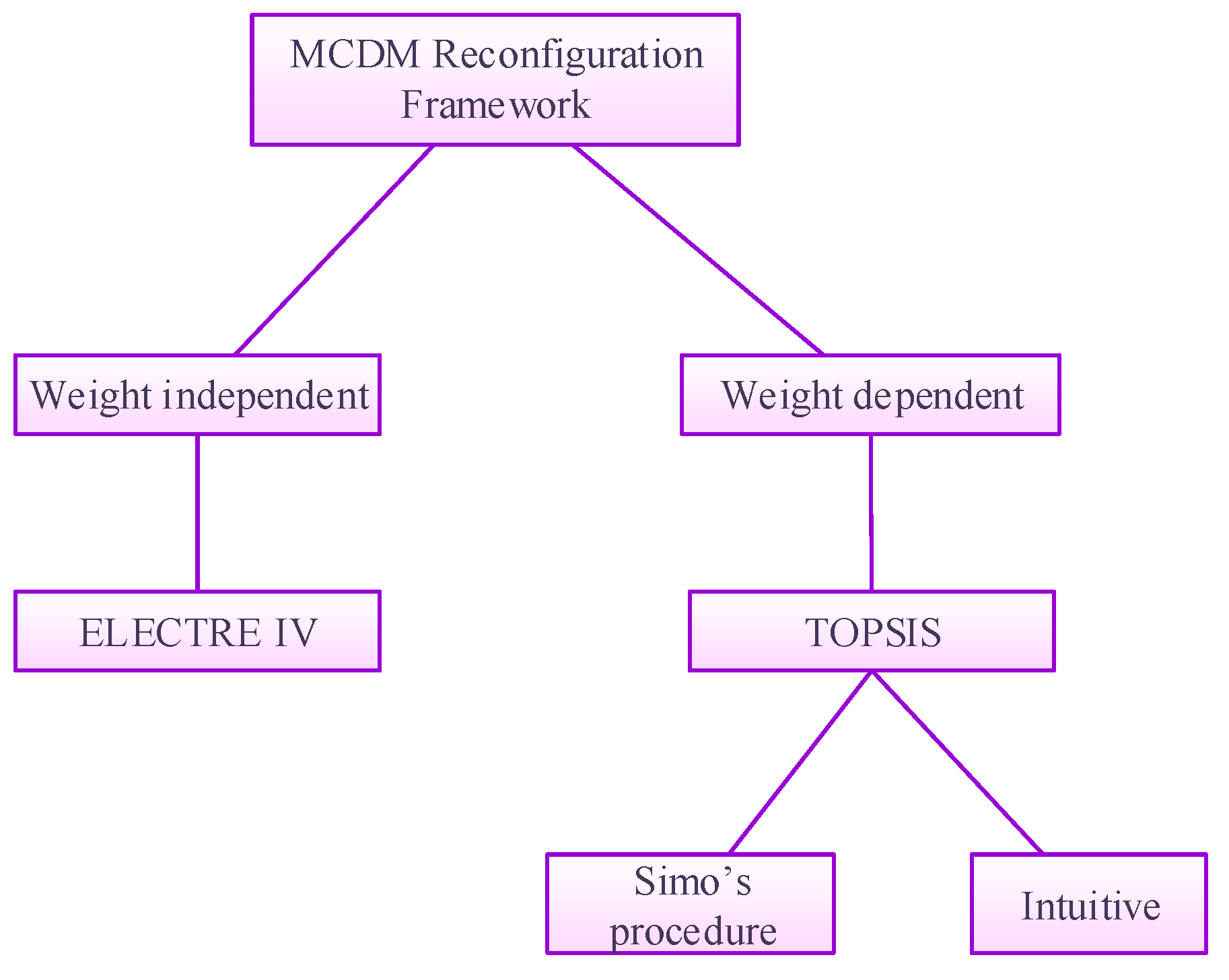
3. MCDM Reconfiguration Framework

The focus of this study is on developing a decision support system (DSS) to help DMs make the best reconfiguration decision during the production execution stage. To cope with changes and disturbances, the DSS assesses a set of capable (candidate) configurations and selects the most suitable one when considering a MCDM approach. To set up the weights of the criteria, we developed three methods convenient to different levels of DM expertise and the desired degree of involvement in the reconfiguration process (see Figure 1):

• intuitive weighting through direct DM involvement;
• indirect weighting through a revised SIMOS procedure weighting; and
• DM (DM) independent weighting.

A set of criteria quantifying numerous aspects of the reconfiguration decision are used to evaluate the candidate configurations. These criteria are categorized into three classes:

• Discrimination criteria are used to evaluate the ability of the configurations to meet the new production requirements, which includes the resource unavailability (RUN) and throughput satisfaction (TS).
• Operational criteria are used to evaluate the dynamic behavior and performance of the candidate configurations, which are composed of two types, namely configuration and resources indicators. The configuration indicators measure the ability of a configuration to meet the current requirements, and resource indicators measure the performance of individual modules.

  Table 1. Operational criteria.

  Configuration Indicators.				Resource Indicators
  Criterion	Notation	Criterion	Notation	Criterion	Notation
  Earliness	ET	Work in Process	WIP	Module Utilization	MU
  Lateness	LT	Nearest to Required Throughput	NRT	No of Modules	NM
  Waiting Time	WT			No operators	NLO

  illustrates these indicators.
• Strategic criteria are used to evaluate the effort (i.e., cost or time) needed to move from the current configuration to a new candidate configuration (i.e., a reconfiguration process). This effort is assessed as a function of the number of removed/added/relocated buffers, machines, and operators.

  Table 2. Strategic indicators.

  Criterion	Notation	Criterion	Notation	Criterion	Notation
  No. of Additional Machines	NAM	No. of Additional Buffers	NAB	No. of Additional Operators	NAO
  No. of Removed Machines	NMM	No. of Removed Buffers	NMB	No. of Removed Operators	NMO
  No. of Relocated Machines	NLM	No. of Relocated Buffers	NLB	No. of Relocated Operators	NLO

  shows these indicators.

The structure of the criteria evaluation framework is shown in Figure 2. More details on these criteria are described in our previous study (Mabkhot et al. [29]).

4. TOPSIS Procedure

TOPSIS was first introduced in 1981 by Hwang et al. [30]. As with many MCDM techniques, TOPSIS compares the available alternatives by normalizing the criterion score, and then finds the so-called “ideal” solution. Next, the geometric distance between the ideal solution and each alternative solution is calculated. The main concept is to choose the alternative that has the shortest and longest distance from a negative and positive ideal solution (PIS and NIS), respectively. TOPSIS is a compensatory aggregation technique that compares all criteria at once rather than using a pairwise comparison, such as in AHP. This type of technique tolerates a trade-off among the criteria, where a good value in one criterion can compensate a poor value of another. Indeed, it enables a more realistic type of modeling not provided by non-compensatory methods, which exclude or include alternatives based on certain cut-offs [31]. In TOPSIS, criteria weights set priorities among the criteria, and indicate preferences to satisfy one criterion over another. The higher a weight is, the more important the criterion. This article does not claim improving the TOPSIS method. Instead, we suggest two ways to assign criteria weights within TOPSIS, namely (1) intuitive weighting based on expert knowledge, and SIMOS weighting.

4.1. Intuitive Weighting

In this method, experts assign weights to prioritize the classes of the criteria. Because the reconfiguration process aims to cope with new production requirements, any configuration that is unable to satisfy these new production requirements should not be considered. The discrimination criteria class examines this ability. Highest priority is given to this class with an accumulative weight of 0.6 (

Table 3. Criteria weights (wj).

Criteria	Discrimination Criteria		Operational Criteria
Indicators	$RUN$	$TS$	$NO$	$NM$	$MU$	$NRT$	LT		ET		$WT$		$WIP$
Value of wj	0.3	0.3	0.03	0.03	0.04	0.04	0.04		0.04		0.04		0.04
Criteria	Strategic Criteria
Indicators	NAM	NMM	NLM	NAB	NMB	NLB		NAO		NMO		NLO
Value of wj	0.0111	0.0111	0.0111	0.0111	0.0111	0.0111		0.0111		0.0111		0.0111

). The next priority is assigned to configurations that meet those requirements with a minimum amount of resources operating with the highest possible utilization rate, which are assessed using the operational criteria class and are given an accumulative weight of 0.3 (Table 3). The least priority is given to the strategic criteria class in which, if more than one configuration has the ability to meet the new requirements with the same operational indicators, the comparison is tackled based on the time and effort needed to move any of those candidate configurations from the current configuration. In fact, this class of criteria assesses the reconfiguration process, which is achieved in real-time, and is given the least priority with an accumulative weight of 0.1 (see the Case study section for the argumentation and discussion). In each class, the weights of the criteria are assigned equally.

4.2. Revised SIMOS Procedure

Assigning the weights of the criteria is an extremely difficult task, particularly for experts who are not used to dealing with the subtleties or intricacies of MCDM techniques. In 1990, Simos [32], [33] developed a new technique that enables any DMs (even without experience in dealing with a MCDM) to express their wishes to assign priority for weights of a variety of criteria. The DM is given a pack of cards and asked simple questions to order the cards, followed by the weights indirectly based on the answers to the questions. This method aims at communicating to MCDM experts the information required for assigning a numerical value to the weights of the criteria. Figueira and Roy [34] revised the original version to overcome some of the method limitations, and Siskos and Tsotsolas [35] improved some of the robustness issues. Within this framework, we revised the method to assign weights to a group of 19 criteria, as shown in Figure 2, for helping DMs with low expertise express their weight preferences.

4.2.1. Collecting the Information

The first step in applying the revised Simos is by writing the name and a short description on a single card for each criterion and using numerous blank cards (more than 4-times the number of named cards). The following steps elaborate on the information collection process:

1-

The name and a brief description of each criterion $g_j, j=1\dots m,$ are written on a card. Hence, there will be $m$ named cards, where $m$ represents the number of criteria (in this case, $m=19$criteria). These cards should not contain any information that can influence the preferences of the DM.

2-

The named cards are given to the DM without any specific arrangement for placement in descending order, starting from the least important cards on the left-hand side and ending with the most important card on the right-hand side (). If the DM believes that two criteria have the same importance, the DM can group them into a subset. In the end, there will be a ranking of the subsets of the criteria $C{S}_r, r=1\dots \overline{m}$; here, $\overline{m}$ represents the number of subsets and $1\le \overline{m}\le m$. As depicted in Figure 3, $C{S}_r$ can be composed of a single criterion, $C{S}_{r=1}$, where rank $r=1$ consists of criterion $g_4$, or can be composed of two or more criteria, i.e., $C{S}_4$, which consists of two criteria $g_{3 }$ and $g_7$.

3-

Until now, any two consecutive subsets $C{S}_r$ and $C{S}_{r+1}$ have an identical distance between them equal to the scale unit $u$ (Figure 3). To help the DM conceive the importance of any two subsets of the criteria, the DM is requested to recognize the distance between them by inserting one or more blank cards. Each inserted blank card is intended to give an extra unit $u$ distance between their weights. For instance, in Figure 3, $C{S}_2$ and $C{S}_3$ have a distance equal to $3u$, which means the latter is $3u$-times more important than the former.

4-

In the end, the DM will be requested to say how much the difference in importance is between the subset on the right-hand side $C{S}_{\overline{m}}$, (the most important) in comparison with the subset on the left-hand side $C{S}_1$ (the least important). In other words, the DM will be asked whether the difference of importance between these two subsets is two-fold, three-fold, or more. This importance value is the Z-ration that determines the absolute value of each player in the evaluation scale.

4.2.2. Algorithm

For each criterion $g_j$, the revised Simos assigns a numerical weight value for $=1,\dots ,m$ according to three steps [35]:

1- Step 1: Assigning non-normalized weights of subsets${\mathit{S}}_{\mathit{r}}$

The non-normalized weight $k_1,\dots ,k_r, \dots , k_{\overline{m}}$ is assigned to subset $C{S}_r$ based on its rank $r$. For this purpose, let $e_r^{\prime }$ represent the number of white cards between ranks $r$ and $r+1$.

Let us define the following:

$$\begin{gathered} {\mathrm{e}}_{\mathrm{r}}{=1+\mathrm{e}}_{\mathrm{r}}^{\prime },\forall \mathrm{r}=1,..,\overline{m}-1 \\ \mathrm{e}={{\displaystyle \sum }}_{\mathrm{r}=1}^{\overline{\mathrm{m}}-1}{\mathrm{e}}_{\mathrm{r}} \\ u=\frac{\mathrm{Z}-1}{\mathrm{e}}\mathrm{retain}\mathrm{six}\mathrm{decimal}\mathrm{places} \end{gathered}$$

(1)

$$\mathrm{Then},k_r=\{\begin{array}{c}1, for r=1\\ 1+u.{\displaystyle {\displaystyle \sum }_{j=1}^{r-1}}{e}_j, \forall \mathrm{r}=2,..\overline{m}-1\end{array}$$

(2)

For $k_r$ weights, we use a rounding-off technique to retain two decimal places.

2- Step 2: Apply criteria non-normalized weights inside a subset$S_r$

Let $\left|C{S}_r\right|$ represent the total number of criteria inside a subset $C{S}_r$. For instance, as shown in Figure 3, $\left|C{S}_{r=3}\right|=3$ (i.e., there are three criteria within $C{S}_{r=3}$, which are $g_8, g_{m-1}\mathrm{and} g_5$), and $\left|C{S}_{r=4}\right|=2$. Each criterion $g_j$ within a subset $C{S}_r$ is assigned the non-normalized weight $k_r$ of subset $C{S}_r$. Let $k_j^{\prime }$ represent the criterion non-normalized weight $g_j$. Then, for each $g_j$ inside a subset $C{S}_r$, $k_j^{\prime }=k_r, \forall j=1, \dots , \left|C{S}_r\right|$. For instance, in Figure 3, $k_{j=8}^{\prime }=k_{j=m-1}^{\prime }=k_{j=5}^{\prime }=k_{r=3}$.

3- Step 3: Convert criteria into normalized weights

The non-normalized weights $k_j^{\prime }, j=1,\dots ,m$ are converted into normalized weights $k_j^{*}$ using Equation (3):

$$k_j^{*}=\frac{100}{K^{\prime }}.k_j^{\prime },\mathrm{where}{K}^{\prime }={{\displaystyle \sum }}_{j=1}^m{k}_j^{\prime }.$$

(3)

In the first released Simos procedure [32,33], the normalized weights $k_j^{*}$ are written without decimal places, where they were rounded into the nearest higher or lower integer value. Nevertheless, Figueira and Roy [34] remarked that these rounding-up techniques in many cases result in a total weight that is less than 100, leading to a distortion. In the MCDM contexts, a distortion is not accepted. To minimize the weight distortion, Figueira and Roy [34] developed the following algorithm:

4.2.3. Rounding and Minimization of Distortion

Figueira and Roy [34] suggest deriving rounded normalized weights $k_j^{\prime \prime }$ from $k_j^{*}$ by either one of three possible options, which is denoted by $\vartheta$ as follows:

$$\{\begin{array}{cc}\vartheta =0:& \mathit{no} \mathit{figures} \mathit{after} \mathit{the} \mathit{decimal} \mathit{point};\\ \vartheta =1:& \mathit{one} \mathit{figure} \mathit{after} \mathit{the} \mathit{decimal} \mathit{point};\\ \vartheta =2:& \mathit{two} \mathit{figures} \mathit{after} \mathit{the} \mathit{decimal} \mathit{point}.\end{array}$$

Using this rounding technique, the following result will be obtained:

$$\{\begin{array}{c}{K}^{″}={\displaystyle \sum }_{j=1}^m{k}_i^{\prime \prime }\le 100,\\ ϵ=100-K^{″}\le {10}^{-\vartheta }\times m.\end{array}$$

(4)

In fact, the value $\tau ={10}^{\vartheta }\times ϵ$ is an integer equal to $m$ at most.

If $k_j=k_j^{\prime \prime }+{10}^{-\vartheta }$ is suitably selected for the $\tau$ criteria and $k_j^{\prime \prime }$ for the remaining $m-\tau$ criteria, ${\displaystyle \sum }_{j=1}^m k_j=100$ will result with normalized weights $k_j$ having the required decimal places [34]. Thus, to obtain the minimum possible distortion of the weights, the $\tau$ criterion in which a value of ${10}^{-\vartheta }$ must be added is determined using the following algorithm [34]:

1- Step 1

For each criterion $g_j$, the following ratios are determined:

$$d_j=\frac{{10}^{-\vartheta }-\left(k_j^{*}-k_j^{\prime \prime }\right)}{k_j^{*}}$$

(5)

which is related to the dysfunction associated with the relative error resulting from rounding up to the nearest integer, and

$$\overline{d_j}=\frac{\left(k_j^{*}-k_j^{\prime \prime }\right)}{k_j^{*}}$$

(6)

which is related to the dysfunction associated with the relative error resulting from rounding downward to the nearest integer.

2- Step 2

Create two lists, $L$ and $\overline{L}$, which are defined as follows:

• List $L$: This is achieved by ranking the pairs of $\left(g_j, d_j\right)$ in increasing values of $d_j$.
• List $\overline{L}$: This is achieved by ranking the pairs of $\left(g_j, \overline{d_j}\right)$ in increasing values of $\overline{d_j}$.
• Set $H=\left\{j/d_j>\overline{d_j}\right\},$and consider $\left|H\right|$ as the number of $g_j$ criteria in set $H$.

3- Step 3

The $m$ criteria are divided into two groups (subsets) $T^{+}$ and $T^{-},$where $\left|T^{+}\right|=\tau$ and $\left|T^{-}\right|=m-\tau$. The $T^{+}$ criteria should be rounded upward to the nearest integer, and in contrast $T^{-}$ should be rounded downward. The division of $T$ is carried out as follows:

(a)

In the case of $\left|H\right|+\tau \le m$, $T^{+}$ is formed with the summation of the $m$ criteria of $H$ and $m-\tau -h$, which represents the last criterion belonging to $\overline{L}$ and not $H$. Thus, list $T^{-}$ is constructed by the first $\tau$ criterion belonging to $\overline{L}$ and not $H$.

(b)

In the case of $\left|H\right|+\tau >m$, $T^{+}$ is formed with the summation $m-h$ criterion belonging to $L$ and not $H$, and $\tau +h-m$, which represents the first criterion belonging to $L$ and not $H.$Thus, list $T^{-}$ is constructed by $m-\tau$, the last criterion belonging to $L$ and not $H$.

The results of these steps will be normalized weights $k_j$. The total sum of these $k_j$ will be 100, which is the aim of the distortion–minimization algorithm. The next step is to convert $k_j$ into $w_j$ and use it in TOPSIS according to the following formula:

$$w_j=k_j/100$$

(7)

Figueira and Roy [34] and Siskos and Tsotsolas [35] fixed some special cases of the revised Simos. The case study section provides a detailed example of the revised Simos to reconfigure the manufacturing systems.

4.3. TOPSIS Algorithm

For an evaluation of $n$ candidate configurations using the $m$ criterion, TOPSIS is accomplished in the following eight steps [31]:

Step 1:

Determine $E= {[x_{ij}]}_{n\times m},$the evaluation matrix of which is as follows:

$$E=\left[\begin{array}{ccc}{x}_{11}& \cdots & x_{1m}\\ ⋮& \ddots & ⋮\\ x_{n1}& \cdots & x_{nm}\end{array}\right],$$

(8)

where $x_{ij}$ represent the performance of indicator j (the third section) in configuration i, assessed based on the new production requirements triggered by a disturbance.

Step 2:

Deduce${[d{m}_{ij}]}_{n\times m}$, the normalized matrix of which is as follows:

$$d{m}_{ij}=x_{ij}/\sqrt{({{\displaystyle \sum }}^{\text{}}{x}_{ij}^2)}.$$

(9)

Step 3:

Calculate $v_{ij},$ the weighted normalized matrix of which is the following:

$$v_{ij}=w_j\times d{m}_{ij},\mathit{where}{{\displaystyle \sum }}^{\text{}}{w}_j=1,\mathit{and}{w}_j\mathit{are}\mathit{set}\mathit{according}\mathit{to}\mathit{Label}\left(16\right).$$

(10)

Step 4:

Let $J_{+}=\left\{j=1,\dots ,f\right\}, 1\le f\le m$, which is related to the set of indicators that have a positive impact, where these indicators are $\left\{RUN,TS,MU,ET\right\}$.

Let $J_{-}=\left\{j=1,\dots ,k\right\}, 1\le k\le m, f+k=m$be related to the set of indicators that have a negative impact, where these indicators are $\left\{NRT,NO,NM,LT,WT,WIP,NAM,NMM,NLM,NAB,NMB,NLB,NAO,NMO,\mathrm{and}NLO\right\}.$

Calculate the row vector $A_P$ of the positive ideal solutions and the row vector $A_N$ of the negative ideal solutions as follows:

$$\begin{gathered} AP=[p{a}_{c_{x}1},\dots ,p{a}_{ij},\dots ,p{a}_{c_{z}m}], \\ \mathit{where}p{a}_{ij}=\{\begin{array}{c}\mathit{max}{v}_{ij} \mathit{over}\mathit{all}\mathit{configurations} i=1,\dots ,n \mathit{and} \forall \mathit{criterion} j\in J_{+};\\ \mathit{min}{v}_{ij} \mathit{over}\mathit{all}\mathit{configurations}i=1,\dots ,n \mathit{and} \forall \mathit{criterion} j\in J_{-}; \end{array} \\ An=[n{a}_{c_{x}1},\dots ,n{a}_{ij},\dots .,n{a}_{c_{z}m}], \\ \mathit{where}n{a}_{ij}=\{\begin{array}{c}\mathit{min}{v}_{ij} \mathit{over}\mathit{all}\mathit{configurations}i=1,\dots ,n \mathit{and} \forall \mathit{criterion} j\in J_{+};\\ \mathit{max}{v}_{ij} \mathit{over}\mathit{all}\mathit{configurations}i=1,\dots ,n \mathit{and} \forall \mathit{criterion} j\in J_{-}; \end{array} \end{gathered}$$

(11)

where $p{a}_{ij}$ and $n{a}_{ij}$ are the best and worst values of criterion j recorded over all configurations.

Step 5:

For each configuration i, calculate distance $S_i^{+}$from the positive ideal solutions and distance $S_i^{-}$ from the negative ideal solutions:

$$S_i^{+}={[{\displaystyle \sum }_{j=1}^m{\left(v_{ij}-p{a}_{ij}\right)}^2]}^{\frac{1}{2}}i=1,\dots ,n$$

(12)

$$S_i^{-}={[{\displaystyle \sum }_{j=1}^m{\left(v_{ij}-n{a}_{ij}\right)}^2]}^{\frac{1}{2}}i=1,\dots ,n$$

(13)

Step 6:

Calculate $C_i$, the relative closeness to the ideal solution.

$$C_i=\frac{S_i^{+}}{S_i^{+}+S_i^{-}},0<C_i<1$$

(14)

Step 7:

Order the configurations based on their relative closeness in ascending order.

Step 8:

Choose the first configuration.

5. ELECTRE IV Procedure

ELECTRE is a non-compensatory technique that uses various mathematical functions to indicate the degree of dominance of one alternative over the others. ELECTRE is a family of variant techniques [37]. Among these variants, ELECTRE IV was derived to deal with such cases in which a DM does not have the required ability, does not like to interfere in a situation, or does not have the knowledge to express the relative importance of the set of criteria. Instead of ranking alternatives (i.e., configurations in our case), ELECTRE IV seeks to establish a partial ordering of alternatives: It groups alternatives that have a similar priority into the same category, and then ranks the categories by introducing the relative order of these categories. ELECTRE IV consists of two phases. First, forming a set of sequences of ranking relations through an alternative pairwise comparison using thresholds. Second, ranking a final-partial preorder that aggregates two complete preorders using an algorithm. As preliminary notations, let us take the following:

• $A=\left\{a_1,a_2,\dots .,a_n\right\}$ as a set of n candidate configurations,
• $F=\left\{g_1,g_2,\dots .,g_m\right\}$ as a set of m criteria, where $m\ge 3$, and
• $g_{\mathrm{j}}(a_i)$ as the performance of the configuration $a_{\mathrm{i}}\in A$ according to the criterion $g_{\mathrm{j}}\in F$.

Figure 4 shows the steps of ELECTRE IV, which will be further illustrated in the following subsections.

5.1. Outranking Relation Constructions

This section presents the set of outranking relations that are exploited to find the final preorders. The thresholds are defined to calculate the preferences and indifferences of the configurations, which are necessary to find the pairwise binary relations used to determine the outranking relations. The outranking relations are the raw data for calculating the fuzzy outranking matrix, which is used along with distillation thresholds as inputs to the ranking algorithm described in the ELECTRE IV section.

5.1.1. Thresholds

In ELECTRE IV, pseudo-criteria are used in place of the real criteria to determine the relations of the fuzzy binary outranking for the configurations. The pseudo-criteria express the DM attitude toward the imprecision, uncertainty, and heterogeneity of the scales. Consider two configurations $a_k$ and $a_n$ that have to be compared. Three thresholds are then defined as follows [38]:

• Indifference threshold$q_{\mathrm{j}}$ refers to the largest difference in the performance between any two configurations $g_j\left(a_k\right)$ and $g_j\left(a_n\right)$ compatible with the situation in which there is no difference.
• Preference threshold$p_j$ refers to the smallest difference in performance between any two configurations $g_j\left(a_k\right)$ and $g_j\left(a_n\right)$ in which the DM undoubtedly prefers an alternative that has the best performance.
• Veto threshold$v{t}_j$ is the smallest difference in performance between any two configurations $g_j\left(a_k\right)$ and $g_j\left(a_n\right)$ according to which the DM is not in favor of the idea that the worst between the two configurations under consideration on a specific criterion may be overall regarded as equivalent to the better one, even when the performance of the worst is better under all other criteria.

The calculation of these thresholds is built on formula 24 [39]:

$$\alpha \times g_j\left(a_i\right)+\beta .$$

(15)

It is a DM’s task to assign values for coefficients $\alpha$ and $\beta$ for all criteria and for each type of threshold. These coefficients must be assigned in such a way that that the resulting thresholds make a clear decision (without a doubt) about an indifference, preference, or veto relation (cf. Section 6 for discussion).

Thresholds can be regarded either in terms of the worst or best performance of two compared configurations. In the former case, the calculation of the thresholds is called “direct,” whereas, in the latter case, the calculation of thresholds is called the “inverse.” The worst performance is considered the smallest if the direction of the preference is increasing (as when evaluating the machine utilization or throughput, for example), and is considered the greatest if the direction of the preference is decreasing (as when evaluating the work in process (WIP), for example).

For example, if $g_j\left(a_k\right)<g_j\left(a_n\right)$ and the direction of preference is increasing, then we have the following:

• The calculation of the direct indifference threshold is $q_j(g_j\left(a_k\right))= \alpha \times g_j\left(a_k\right)+\beta$.
• The calculation of the inverse indifference threshold is $q_j(g_j\left(a_k\right))=\alpha \times g_j\left(a_n\right)+\beta$.

For the same case, but with a decreasing preference, we have the following:

• The direct indifference threshold will be calculated as $q_j(g_j\left(a_n\right))=\alpha \times g_j\left(a_n\right)+\beta$.
• The inverse indifference threshold will be calculated as $q_j(g_j\left(a_n\right))=\alpha \times g_j\left(a_k\right)+\beta$.

Therefore, the calculation of the thresholds is based on four cases:

• Case 1: Increasing the preferences for the performance (↑) and direct thresholds (→).
• Case 2: Decreasing the preferences for the performance (↓) and direct thresholds (→).
• Case 3: Increasing the preferences for the performance (↑) and inverse thresholds (←).
• Case 4: Decreasing the preferences for the performance (↓) and inverse thresholds (←).

For any case, $\alpha$ and $\beta$ coefficients must not bring back a negative value for a threshold. Then, to guarantee consistency [39], consider the following:

• In Case 1, the coefficient is $\alpha \ge -1$.
• In Cases 2 and 3, the coefficient is $\alpha <1$.
• In Case 4, the coefficient is $\alpha >-1$.
• The following relation should be satisfied for each criterion: $q_j(.)\le p_j(.)\le v{t}_j(.)$.
• To avoid an incoherence, the following conditions should be satisfied:

  $$\frac{q_j(g_j\left(a_n\right))-q_i(g_j\left(a_k\right))}{g_j\left(a_n\right)-g_j\left(a_k\right)}\ge -1$$

  (16)

  $$\frac{p_j(g_j\left(a_n\right))-p_i(g_j\left(a_k\right))}{g_j\left(a_n\right)-g_j\left(a_k\right)}\ge -1$$

  (17)

  $$\frac{v{t}_j(g_j\left(a_n\right))-v_i(g_j\left(a_k\right))}{g_j\left(a_n\right)-g_j\left(a_k\right)}\ge -1$$

  (18)

5.1.2. Preferences and Indifferences

Situations of strict preference, weak preference, and indifference are defined according to Equations (19)–(21) [40]:

$$a_n{\mathit{I}}_j{a}_k\iff g_j\left(a_n\right)-g_j\left(a_k\right)<q_i(g_j\left(a_k\right))$$

(19)

$$a_n{\mathit{P}}_j{a}_k\iff p_i(g_j\left(a_k\right))<g_j\left(a_n\right)-g_j\left(a_k\right)$$

(20)

$$a_n{\mathit{Q}}_j{a}_k\iff q_i(g_j\left(a_k\right))<g_j\left(a_n\right)-g_j\left(a_k\right)\le p_i(g_j\left(a_k\right))$$

(21)

where, $a_k{\mathit{I}}_j{a}_n$, refers to a situation in which the DM is indifferent between configurations $a_k$ and $a_n$, $a_k{\mathit{P}}_j{a}_n$, refers to a situation in which configuration $a_k$ is strictly preferred over configuration $a_n$, and $a_k{\mathit{Q}}_j{a}_n$ refers to a situation in which configuration $a_k$ is weakly preferred over configuration $a_n$.

5.1.3. Pairwise Binary Relations

The binary relations for any pair of configurations $\left(a_k, a_n\right)$ is calculated as follows [39]:

$$\mathit{m}=m_p\left(a_k,a_n\right)+m_q\left(a_k,a_n\right)+m_i\left(a_k,a_n\right)+m_0\left(a_k,a_n\right)+m_p\left(a_n,a_k\right)+m_q\left(a_n,a_k\right)+m_i\left(a_n,a_k\right).$$

(22)

where, ${\mathit{m}}_{\mathit{p}}\left({\mathit{a}}_{\mathit{k}},{\mathit{a}}_{\mathit{n}}\right)$, represents the number of criteria when configuration $a_k$ is strictly preferred over configuration $a_n$, ${\mathit{m}}_{\mathit{q}}\left({\mathit{a}}_{\mathit{k}},{\mathit{a}}_{\mathit{n}}\right)$, represents the number of criteria when configuration $a_k$ is weakly preferred over configuration $a_n$, ${\mathit{m}}_{\mathit{i}}\left({\mathit{a}}_{\mathit{k}},{\mathit{a}}_{\mathit{n}}\right)$, represents the number of criteria when the DM is indifferent between configurations $a_k$ and $a_n$, and ${\mathit{m}}_{\mathit{o}}\left({\mathit{a}}_{\mathit{k}},{\mathit{a}}_{\mathit{n}}\right)$, represents the number of criteria when configuration $a_k$ has the same evaluation as $a_n$.

If two relations exist for the same criteria $a_k$ and $a_n$, the richest/dominated one will be considered. The order of relations from lowest to highest in richness is $S_q\subset S_c\subset S_p\subset S_s\subset S_v$. This means that $S_v$ dominates all four relations, and $S_s$ dominates $S_q, S_c, S_p$, …, etc. For instance, if the two relations $a_k {\mathit{S}}_{\mathit{q}} a_n$ and$a_k {\mathit{S}}_{\mathit{s}} a_n$ exist, the $a_k {\mathit{S}}_{\mathit{s}} a_n$relation dominates$a_k {\mathit{S}}_{\mathit{q}} a_n$, and it will be considered (cf. Section 6 for an example).

5.1.4. Outranking Relations

The outranking relations for ELECTRE IV are defined as follows [41]:

Quasi-dominance ${\mathit{S}}_{\mathit{q}}$	$\mathit{I}\mathit{f}{m}_p\left(a_n,a_k\right)+m_q\left(a_k,a_n\right)=0$ $\mathit{a}\mathit{n}\mathit{d}{m}_i\left(a_n,a_k\right)<m_i\left(a_k,a_n\right)+m_q\left(a_k,a_n\right)+m_p\left(a_k,a_n\right)$ $\mathit{t}\mathit{h}\mathit{e}\mathit{n}{a}_k{\mathit{S}}_{\mathit{q}}{a}_n$;
Canonic-dominance ${\mathit{S}}_{\mathit{c}}$	$\mathit{I}\mathit{f}{m}_p\left(a_n,a_k\right)=0$ $\mathit{a}\mathit{n}\mathit{d}{m}_q\left(a_n,a_k\right)\le m_p\left(a_k,a_n\right)$ $\mathit{a}\mathit{n}\mathit{d}{m}_q\left(a_n,a_k\right)+m_i\left(a_n,a_k\right)<m_i\left(a_k,a_n\right)+m_q\left(a_k,a_n\right)+m_p\left(a_k,a_n\right)$ $\mathit{t}\mathit{h}\mathit{e}\mathit{n}{a}_k{\mathit{S}}_{\mathit{c}}{a}_n$;
Pseudo-dominance ${\mathit{S}}_{\mathit{p}}$	$\mathit{I}\mathit{f}{m}_p\left(a_n,a_k\right)=0$ $\mathit{a}\mathit{n}\mathit{d} m_q\left(a_n,a_k\right)\le m_q\left(a_k,a_n\right)+m_p\left(a_k,a_n\right)$ $\mathit{t}\mathit{h}\mathit{e}\mathit{n}{a}_k{\mathit{S}}_{\mathit{p}}{a}_n$;
Sub-dominance ${\mathit{S}}_{\mathit{s}}$	$\mathit{I}\mathit{f}{m}_p\left(a_n,a_k\right)=0$ $\mathit{t}\mathit{h}\mathit{e}\mathit{n}{a}_k{\mathit{S}}_{\mathit{s}}{a}_n$;
Veto-dominance ${\mathit{S}}_{\mathit{v}}$	$\mathit{I}\mathit{f}{m}_p\left(a_n,a_k\right)=0$ $\mathit{o}\mathit{r}\{\begin{array}{c}{m}_p\left(a_n,a_k\right)=1 \\ m_p\left(a_k,a_n\right)\ge \frac{m}{2} \\ g_j\left(a_k\right)+v{t}_j\left(g_j\left(a_k\right)\right)\ge g_j\left(a_n\right), \forall j\in F\end{array}$ $\mathit{t}\mathit{h}\mathit{e}\mathit{n}{a}_k{\mathit{S}}_{\mathit{v}}{a}_n$.

5.1.5. Fuzzy Outranking Matrix

For each pair $\left(a_n, a_k\right)$ of configurations, a credibility degree $\sigma \left(a_n, a_k\right)\in \left[0,1\right]$ indicates how much configuration $\left(a_n\right)$ outranks the configuration $\left(a_k\right)$[40]:

$$\sigma (a_n,a_k)=\{\begin{array}{cc}1& if{a}_n{S}_q{a}_k\\ 0.8& if{a}_n{S}_c{a}_k\\ 0.6& if{a}_n{S}_p{a}_k\\ 0.4& if{a}_n{S}_s{a}_k\\ 0.2& if{a}_n{S}_v{a}_k\\ 0& ifnorelationamong\{S_q,S_c,S_p,S_s,S_v\}\end{array}$$

(23)

Credibility degrees are used to determine the matrix of the fuzzy outranking:

Fuzzy outranking matrix =	$\mathit{\sigma }\left(.,.\right)$	${\mathit{a}}_{\mathbf{1}}$	${\mathit{a}}_{\mathbf{2}}$	.	.	${\mathit{a}}_{\mathit{n}}$	(24)
	${\mathit{a}}_{\mathbf{1}}$	1	$\sigma \left(a_1,a_2\right)$	$\sigma \left(a_1,.\right)$	$\sigma \left(a_1,.\right)$	$\sigma \left(a_1,a_k\right)$
	${\mathit{a}}_{\mathbf{2}}$	$\sigma \left(a_2,a_1\right)$	1	$\sigma \left(a_2,.\right)$	$\sigma \left(a_2,.\right)$	$\sigma \left(a_1,a_k\right)$
	.	$\sigma \left(.,a_1\right)$.	$\sigma \left(.,a_2\right)$	1	$\sigma \left(.,.\right)$	$\sigma \left(.,a_k\right)$
	.	$\sigma \left(.,a_1\right)$	$\sigma \left(.,a_2\right)$	$\sigma \left(.,.\right)$	1	$\sigma \left(.,a_k\right)$
	${\mathit{a}}_{\mathit{n}}$	$\sigma \left(.,a_1\right)$	$\sigma \left(a_n,a_2\right)$	$\sigma \left(a_n,.\right)$	$\sigma \left(a_n,.\right)$	1

5.1.6. Distillation Threshold

From the fuzzy outranking matrix, a succession of crispy outranking relations is constructed. To do so, a set of cutoff levels $({\lambda }_l)\in \left[0,1\right]$ and a distillation threshold $s\left({\lambda }_l\right)$ are defined. The distillation threshold is calculated as follows:

$$s\left({\lambda }_l\right)=\delta \times {\lambda }_l+\gamma$$

(25)

Then, only the arcs $a_n \mathrm{and} a_k$ of the fuzzy outranking relation for which $\sigma \left(a_n, a_k\right)>{\lambda }_l$ are held, and a crispy outranking relation $S_A^{{\lambda }_l}$, can be calculated as follows:

$$S_A^{{\lambda }_l}\iff \{\begin{array}{c}\sigma \left(a_n,a_k\right)>{\lambda }_l \\ \sigma \left(a_n,a_k\right)>\sigma \left(a_k,a_n\right)+s\left(\sigma \left(a_n,a_k\right)\right) \end{array}$$

(26)

This means that the declaration “$a_n$ outranks $a_k$” will be considered if it is more significant than the reverse declaration “$a_k$ outranks $a_n$.” The distillation threshold function is constant, where $\delta = 0$ and $\gamma = 0.1$. Thus, $s\left(\lambda \right)=0.1$. This value permits the transformation of a nested relation into a fuzzy one. Because of the ranking, we have the following:

• In the first step, only the strongest dominance threshold among those that have been asserted will be considered.
• In the second step, the two strongest dominance thresholds will be considered.

From the crispy outranking matrix, the calculations are made for all configurations [39]:

• ${\mathit{\lambda }}_{\mathit{l}}-\mathit{p}\mathit{o}\mathit{w}\mathit{e}\mathit{r} ofconfiguration{a}_n$: $p_A^{{\lambda }_l}\left(a_n\right)$determines the number of configurations that $a_n$ outranks:

  $$p_A^{{\lambda }_l}\left(a_n\right)=|\{a_k\in A/a_n{S}_A^{{\lambda }_l}\left(a_k\right)\left\}\right|$$

  (27)
• ${\mathit{\lambda }}_{\mathit{l}}-\mathit{w}\mathit{e}\mathit{a}\mathit{k}\mathit{n}\mathit{e}\mathit{s}\mathit{s} ofconfiguration{a}_n$: $f_A^{{\lambda }_l}$($a_n)$determines the number of configurations that outrank $a_n$:

  $$f_A^{{\lambda }_l}\left(a_n\right)=|\{a_k\in A/a_k{S}_A^{{\lambda }_l}\left(a_n\right)\left\}\right|$$

  (28)
• ${\mathit{\lambda }}_{\mathit{l}}-\mathit{q}\mathit{u}\mathit{a}\mathit{l}\mathit{i}\mathit{f}\mathit{i}\mathit{c}\mathit{a}\mathit{t}\mathit{i}\mathit{o}\mathit{n} ofconfiguration{a}_n$: $q_A^{{\lambda }_l}$($a_n)$ determines the relative rank of configuration $a_n$ in set $A$:

  $$q_A^{{\lambda }_l}\left(a_n\right)=p_A^{{\lambda }_{\mathrm{l}}}\left(a_n\right)-f_A^{{\lambda }_l}\left(a_n\right)$$

  (29)

5.2. Ranking Algorithm

Using the fuzzy outranking matrix (Equation (24)), a ranking algorithm is deployed to order the candidate configurations in two complete pre-orders. The two pre-orders are accomplished through several iterations called distillations. The first pre-order, descending, results in a descending order, starting with the best configuration. The second pre-order, ascending, results in an ascending manner, starting with the worst configuration.

5.2.1. Distillation

Let ${\lambda }_l$ be the first cutoff level and $q_A^{{\lambda }_k}\left(a_n\right)$ be the qualification of configuration $a_n$. Then, in set $A$ of the candidate configurations, the best configuration(s) that have the maximum qualification in the descending selection will be denoted as a subset ${\overline{D}}_1,$and the worst configuration(s) that have the minimum qualification in the ascending selection will be denoted as a subset ${\underset{\_}{D}}_1$. These two subsets are calculated as follows:

$${\overline{D}}_1=\left\{a_n\in A⁄q_A^{{\lambda }_1}\left(a_n\right)={\overline{q}}_A=\underset{x\in A}{max}{q}_A^{{\lambda }_1}\left(x\right)\right\}$$

(30)

$${\underset{\_}{D}}_1=\left\{a_n\in A⁄q_A^{{\lambda }_1}\left(a_n\right)={\underset{\_}{q}}_A=\underset{x\in A}{min}{q}_A^{{\lambda }_1}\left(x\right)\right\}$$

(31)

Hence, at the end of $l$ steps of the first distillation, the first subset of $A$, which will contain the first/last class of one of the two final pre-orders, is selected.

Let ${\overline{C}}_1= {\overline{D}}_1$ represent the first class of the descending selection, and ${\underset{\_}{C}}_1= {\underset{\_}{D}}_1$ represent the first class of the ascending selection. Thus, $A_1=A\backslash {\overline{C}}_1$ or $A_1=A\backslash {\underset{\_}{C}}_1$ represents the remaining subset of configurations from $A$ to be ranked after the first distillation. To select one or more configuration, in this subset, the qualification of each configuration will be calculated again. This step will be reiterated until all configurations are ranked.

5.2.2. Ascending and Descending Pre-Ordering Algorithms.5.2.3. Final Ranking

Step-1:	$y=0,{\overline{A}}_0=A\mathit{o}\mathit{r}{\underset{\_}{A}}_0=A.$
Step-2:	${\lambda }_0=\underset{a_n,a_k\in {\overline{A}}_{y,n\ne k}}{\max }\sigma \left(a_n,a_k\right)\mathit{o}\mathit{r}{\lambda }_0=\underset{a_n,a_k\in {\underset{\_}{A}}_{y,n\ne k}}{\min }\sigma \left(a_n,a_k\right)$
Step-3:	$l=0,D_0={\overline{A}}_y\mathit{o}\mathit{r}{D}_0={\underset{\_}{A}}_0.$
Step-4:	Among the arcs of the fuzzy outranking relations that have credibility lower than ${\lambda }_l-s\left({\lambda }_l\right)$, select the one with the maximum value: ${\lambda }_{l+1}=\underset{\sigma \left(a_n,a_k\right)>{\lambda }_l-s\left({\lambda }_l\right)\},n\ne k}{\max }\sigma \left(a_n,a_k\right)$ Notice that $\forall a_n,a_k\in D_l,\sigma \left(a_n,a_k\right)>{\lambda }_l-s\left({\lambda }_l\right)\Rightarrow {\lambda }_{l+1}=0.$
Step-5:	Calculate the ${\lambda }_l-qualifications$ of all configurations belonging to $D_l$.
Step-6:	Obtain the minimum or maximum ${\lambda }_l-qualifications$: ${\overline{q}}_{D_l}$, or ${\underset{\_}{q}}_{D_l}$.
Step-7:	Build the subset: ${\overline{D}}_{l+1}=\left\{a_n\in D_l⁄q_{D_l}^{{\lambda }_{k+1}}\left(a_n\right)={\overline{q}}_{D_l}\right\}$, or ${\underset{\_}{D}}_{l+1}=\{a_n\in D_l⁄q_{A{D}_l}^{{\lambda }_{k+1}}\left(a_n\right)={\underset{\_}{q}}_{D_l}$
Step-8:	if$\left|{\overline{D}}_{l+1}\right|=1$or$\left|{\underset{\_}{D}}_{l+1}\right|=1$ or ${\lambda }_{l+1}=0$then, go to step 9 else, do $l=l+1$, $D_l$ = ${\overline{D}}_l$ or $D_l$ = ${\underset{\_}{D}}_l$, go to step 4
Step-9:	${\overline{C}}_{y+1}={\overline{D}}_{y+1}or{\underset{\_}{C}}_{y+1}={\underset{\_}{D}}_{y+1}$ do${\overline{A}}_{y+1}$ =${\overline{A}}_y\backslash {\overline{C}}_{y+1}$ or ${\underset{\_}{A}}_{y+1}$ =${\underset{\_}{A}}_y\backslash {\underset{\_}{C}}_{y+1}$ if ${\overline{A}}_{y+1}=\varnothing$ or ${\underset{\_}{A}}_{y+1}=\varnothing$ then $y=y+1$, go to step 2 else, END of distillation.

At the end of ascending and descending pre-orders, the result will be two complete pre-orders. In each of them, the configurations will be grouped in a set of ranked classes. Each class consists of at least one configuration. To obtain the intersection pre-order (the final order), the following rules are applied:

• Configuration $a_n$ is considered better than $a_k$ if in at least one of the distillations, $a_n$ is better than $a_k$, and in the other distillation, $a_n$ is at least as well ranked as $a_k$.
• Configuration $a_n$ is judged as indifferent to $a_k$ if the two configurations belong to the same equivalence class in the two pre-orders.
• Configuration $a_n$ and $a_k$ are incomparable if $a_n$ is better ranked than $a_n$ in the ascending distillation and $a_k$ is better ranked than $a_k$ in the descending distillation, or vice-versa.

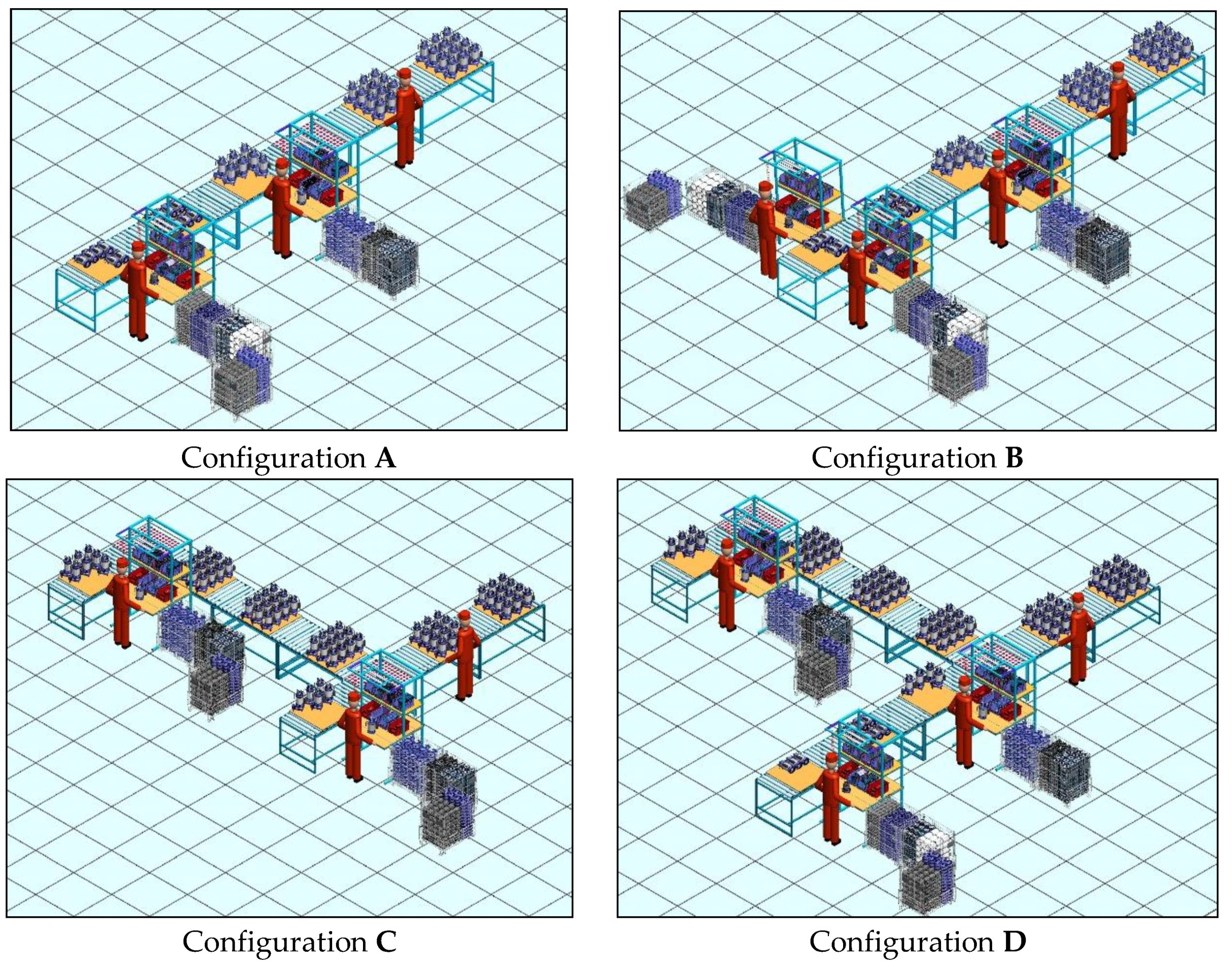
6. Case Study

This section presents a case study and illustrates how to use the decision-making framework to select a configuration that can best meet the current situation.

6.1. Presentation of the Case Study

In this study, we consider an electro-mechanical manufacturing plant that assembles electro-submersible pumps (ESP) with a variety of power, sizes, and usages. An ESP is an artificial technique for pumping up high to moderate volumes of fluids (e.g., sewage and drainage waters) from wells. Submersible pumps are manufactured in different pressure heads that range between 7 to 50 m and flow rates of between 10 and 2500 m³/h. An ESP assembly is applied in semi-automated assembly lines. DMs can reconfigure the assembly lines by adding, removing, and/or relocating modules during the production running time, which enables an easy and quick adaption of product functionality and capacity against risks and disturbances. Each configuration differs in the number of modules, module arrangement, and/or worker assignment to the modules. One or two skilled operators are required to accomplish the assembly task on each module. Basic modules can serve numerous purposes, such as inspection, assembly, delivery, and packaging. The performance of each module differs from one task to another based on the type of accomplished task, the type of product, and operator skills (Figure 5).

Four configurations (A, B, C, and D) are provided in Figure 5 to illustrate the physical implementation of the configurations on the shop floor. The presentation of these four configurations is for the sake of harmonizing the description of the case study with the illustration of the reconfiguration example elaborated in Section 6.1.2.

We represent the discrete layout of the shop floor as a grid by dividing it into rows and columns. Each configuration component can be assigned to a location on the grid, which describes the physical implementation of the configuration resources on the shop floor. A different assignment of workers to the modules yields a different configuration.

6.1.1. Simulation-Based Evaluation of Configurations

To evaluate the criteria for each configuration, we gathered data from a real case study and implemented it in ARENA simulation software version 15.1. Over a 6-day period (one 8 h shift a day), we collected data to generate the service time distributions. The ARENA Input Analyzer is used for this purpose, and simulation results directly provide values for most of the operational criteria, as shown in

Table 4. Performance indicators of configurations.

Configuration	NO	NM	MU (%)	Th (Pcs/day)	WT (Hrs)	WIP (Pcs)
A	3	3	0.67	60	1.40	11.12
B	4	4	0.72	96	1.89	21.05
C	3	3	0.62	80	1.10	8.90
D	4	4	0.79	108	1.39	13.80

, whereas the discrimination, strategic, and other operational criteria are calculated from these criteria based on the equations illustrated in Section 3. Calculating the values of the criteria related to RUN, TS, ET, LT, and NRT relies on the performance indicators, in addition to the production order, leading to a change in the running configuration.

Table 5. Simulation parameters.

Modules	Service Times (minute)
	Motor Assembly	Pump Assembly	Electro-Submersible Assembly
Module-1	NORM(7.01, 0.374)	LOGN(4.95, 0.559)	LOGN(12.51, 0.86)
Module-2	6.4 + GAMM(0.331,3.82)	3.69 + GAMM(0.451, 4.12)	12 + GAMM(0.331, 3.82)
Module-3	LOGN(6.5.22, 0.857)	NORM(5, 0.23)	LOGN(11.55, 0.343)
Module-4	NORM(7.3, 0.005)	LOGN(5.2, 0.603)	LOGN(12.4, 0.902)
Inspection	UNIF(2, 25)

shows the generated distributions. The inter-arrival times of the parts are based on the availability of the first module on the line, where the parts are available in mesh baskets and can enter the assembly line immediately after dispatching the previous part. The transportation time between modules is determined based on the speed of the roll conveyor, which has a maximum speed of 42 m/min and is controlled by the next module operator. We built and verified a model for each configuration under normal operating conditions. The simulation models ran for 100 replications each 11 h long with a 3 h warm up.

The simulation results directly provide values for most of the operational criteria, as shown in Table 4, whereas the discrimination, strategic, and other operational criteria are calculated from these criteria based on the equations illustrated in Section 3. Calculating the values of the criteria related to RUN, TS, ET, LT, and NRT relies on the performance indicators, in addition to the production order, leading to a change in the running configuration.

A strategic criteria calculation based on the amount of change will be carried out on the assignments and physical locations of the modules and operators to move to each candidate configuration.

6.1.2. Disturbance Occurrence

Let us consider configuration A to be currently in operation to assemble an order, in which 420 pieces of product ESP 0.5 HP are due after seven working days, where the factory operates a single 8 h shift. Any configuration having a throughput Th of more than or equal to 60 Pcs/day is able to meet the order on time. As we can see from

Table 6. Relative closeness to ideal solution, intuitively weighting based.

Configurations	${\mathit{S}}_{\mathit{i}}^{+}$	${\mathit{S}}_{\mathit{i}}^{-}$	${\mathit{C}}_{\mathit{i}}$	Rank
D	0.0005719	0.6740291	0.0008477	1
B	0.0011098	0.6855460	0.0016163	2
C	0.0465463	0.6313395	0.0686639	3

, configuration A is capable of accomplishing this order on time under normal conditions, where Th is equal to 60 Pcs/day. At some point, a disturbance occurs, in which Module_02 fails, affecting the performance of the configuration and its ability to meet the orders on time. The consequences of the disturbance can be determined using approaches, such as described in [42]. Now, a reconfiguration decision has to be made. The DM has to decide whether to continue using configuration A or move to another configuration. In this latter case, the DM has to decide which configuration to use (i.e., B, C, or D, all of which are feasible).

6.2. TOPSIS Selection

An expert from the factory who is in charge of taking the reconfiguration decision is selected to implement the framework. He has more than twenty years of experience as ESP production supervisor and manager. The same expert opinion was used to implement the three methods of the framework (cf. Section 4.1 and Section 4.2.1). The following subsections illustrate the application of TOPSIS using the two different weighting methods.

6.2.1. Intuitive Weighting

This section shows the implementation of TOPSIS based on the intuitive weighting method described in Section 4.1.

Step 1: Determine $E= {[x_{ij}]}_{n\times m},$the evaluation matrix of which is as follows:

	RUN	TS	NO	NM	MU	ET	LT	NRT	WT	WIP	NAM	NMM	NLM	NAB	NMB	NLB	NAO	NMO	NLO
E=	1	1	4	4	0.79	2	0	44	1.39	13.80	1	0	0	4	0	0	1	0	0	Config D
	0	1	3	3	0.62	0	0	16	1.1	8.9	1	1	0	3	0	1	1	1	0	Config C
	1	1	4	4	0.72	1	0	32	1.89	21.05	2	1	0	0	0	0	2	1	0	Config B

Step 2: Deduce the normalized decision matrix${(r_{ij})}_{n\times m}$.

$$d{m}_{ij}=\left[\begin{array}{ccccccc}0.71& 0.58& 0.62& \cdots & 0.41& 0& 0\\ 0& 0.58& 0.47& \cdots & 0.41& 0.71& 0\\ 0.71& 0.58& 0.62& \cdots & 0.82& 0.71& 0\end{array}\right]$$

Step 3: Calculate $v_{ij},$ the weighted normalized matrix of which is as follows:

$$v_{ij}=\left[\begin{array}{ccccccc}0.212& 0.17& 0.019& \cdots & 0.004& 0& 0\\ 0& 0.17& 0.014& \cdots & 0.004& 0.007& 0\\ 0.212& 0.17& 0.019& \cdots & 0.008& 0.007& 0\end{array}\right]$$

Step 4: Calculate the positive and negative ideal solutions $\left(A_P\right) \mathrm{and} \left(A_N\right)$:

$$\begin{gathered} {\mathrm{A}}_P= \left[0.212 0.17 0.014 \dots 0.004 0 0\right] \\ {\mathrm{A}}_N= \left[0 0.17 0.019 \dots 0.008 0.007 0\right] \end{gathered}$$

Steps 5, 6, 7, and 8: Determine the positive and negative ideal solutions $(S_i^{+}) \mathrm{and} \left(S_i^{-}\right)$, and the relative closeness to the ideal solution$C_i.$ Rank the candidate configurations in ascending order and choose the configuration that ranks at the top.

Table 6 shows that configuration D is ranked at the top of the list (${\mathrm{C}}_{\mathrm{i}}$ = 0.0008477), followed by configuration B (${\mathrm{C}}_{\mathrm{i}}=$0.0016163) and configuration C (${\mathrm{C}}_{\mathrm{i}}$ = 0.0686639).

6.2.2. Improved SIMOS Weighting

This section demonstrates the use of the improved SIMOS method to assign the weight and the use of this weight in TOPSIS. First, we implement SIMOS (cf. Section 4.2) for the same case study.

Collecting the Information:

We have $m$ = 19 criteria, and the DM orders them from least to most important. The DM forms 14 subsets $S{C}_{r }$ of criteria $\overline{m}$. Thirteen white cards are inserted between the subsets of the criteria. In addition, the DM sets up $z=24$, which is the ratio between the least important $\left(NMO\right)$ to the most important ($RUN)$ criterion. The results of the collection are depicted in the first three columns of

Table 7. Non-normalized weights for z = 24.

Rank (Ascending)	$\mathbf{Subset}\mathbf{of}\mathbf{Criteria}\mathit{S}{\mathit{C}}_{\mathit{r} }$	$\mathbf{Number}\mathbf{of}\mathbf{White}\mathbf{Cards}\mathbf{According}\mathbf{to}\mathit{r}$$\mathbf{and}{\mathit{e}}_{\mathit{r}}^{\prime }$	${\mathit{e}}_{\mathit{r}}$	$\mathbf{Non}-\mathbf{Normalized}\mathbf{Weights}\mathbf{k}\left(\mathit{r}\right)$	Total
1	NMO	0	1	1	1.00
2	NMB, NMM	1	2	1.85	3.70
3	NLO	0	1	3.56	3.56
4	NLB, NLM	1	2	4.41	8.81
5	NAO	0	1	6.11	6.11
6	NAB, NAM	1	2	6.96	13.93
7	NO	1	2	8.67	8.67
8	NM, MU	1	2	10.37	20.74
9	ET	0	1	12.07	12.07
10	WT, WIP	1	2	12.93	25.85
11	NRT	1	2	14.63	14.63
12	LT	6	7	16.33	16.33
13	TS	0	1	22.30	22.30
14	RUN	0	1	23.15	23.15
Sum	19	13	27	…	180.85

.

The algorithm:

Step 1: Determine the non-normalized weights as follows: $e=27$, and thus $u=\frac{24-1}{27}=0.851852$, and the non-normalized weights $k\left(r\right)$ are as shown in Table 7.

Step 2: Determine the normalized weights as follows: The three normalized weights $k_j^{*}$, $k_j^{\prime \prime }$, and $k_j$ are shown in

Table 8. Normalized weights for w = 1 and z = 24.

Rank	Criteria	N.	$\mathbf{Normalized}\mathbf{Weights}{\mathit{k}}_{\mathit{j}}^{*}$	$\mathbf{Normalized}\mathbf{Weights}{\mathit{k}}_{\mathit{j}}^{\prime \prime }$	$\mathbf{Ratio}{\mathit{d}}_{\mathit{j}}$	$\mathbf{Ratio}\overline{{\mathit{d}}_{\mathit{j}}}$	$\mathbf{Normalized}\mathbf{Weights}{\mathit{k}}_{\mathit{j}}$
1	NMO	18	0.553	0.5	0.085	0.096	0.5
2	NMB	15	1.024	1.0	0.074	0.023	1.1
2	NMM	12	1.024	1.0	0.074	0.023	1.1
3	NLO	19	1.966	1.9	0.017	0.034	1.9
4	NLB	16	2.437	2.4	0.026	0.015	2.5
4	NLM	13	2.437	2.4	0.026	0.015	2.5
5	NAO	17	3.379	3.3	0.006	0.023	3.3
6	NAB	14	3.850	3.8	0.013	0.013	3.8
6	NAM	11	3.850	3.8	0.013	0.013	3.8
7	NO	3	4.792	4.7	0.002	0.019	4.7
8	NM	4	5.734	5.7	0.011	0.006	5.8
8	MU	5	5.734	5.7	0.011	0.006	5.8
9	ET	6	6.676	6.6	0.004	0.011	6.6
10	WT	9	7.147	7.1	0.007	0.007	7.2
10	WIP	10	7.147	7.1	0.007	0.007	7.2
11	NRT	8	8.089	8.0	0.001	0.011	8.0
12	LT	7	9.031	9.0	0.008	0.003	9.1
13	TS	2	12.328	12.3	0.006	0.002	12.4
14	RUN	1	12.800	12.7	0.00004	0.008	12.7
SUM	19	…	100	99	…	…	100.0

, where $K_j^{\prime \prime }$ is equal to 99, and $ϵ=100-99=1$, and $\tau ={10}^1*1=10$.

Rounding and Minimization of Distortion

The two ratios $d_j$ and $\overline{d_j}$ are shown in columns 7 and 8 of Table 8, respectively. In addition, $\left|H\right|=$10 and $\left|H\right|+\tau =20>m=19$, and $T^{+}$ criteria will then be deduced using the second rule (the TOPSIS section). The two lists of $\overline{L}$ and two subsets of $T^{+}$ and $T^{-}$ are shown in

Table 9. Lists if L, L, T+, and T− for ϑ =1.

N. Crit.	$\mathit{L}$	N. Crit.	$\overline{\mathit{L}}$	N. Crit.	${\mathit{T}}^{-}$
1	0.00004	18	0.096	1	√
8	0.001	19	0.034	8	√
3	0.002	17	0.023	3	√
6	0.004	15	0.023	6	√
2	0.006	12	0.023	2
17	0.006	3	0.019	17	√
9	0.007	16	0.015	9
10	0.007	13	0.015	10
7	0.008	14	0.013	7
4	0.011	11	0.013	4
5	0.011	6	0.011	5
14	0.013	8	0.011	14	√
11	0.013	1	0.008	11	√
19	0.017	9	0.007	19	√
16	0.026	10	0.007	16
13	0.026	4	0.006	13
15	0.074	5	0.006	15
12	0.074	7	0.003	12
18	0.085	2	0.002	18	√

.

The resulting weights from the SIMOS procedure are shown in

Table 10. Weights of the criteria based on the SIMOS procedure.

Criteria	Discrimination Criteria		Operational Criteria
Indicators	$RUN$	$TS$	$NO$	$NM$	$MU$	$NRT$	LT		ET		$WT$		$WIP$
Value of wj	0.127	0.124	0.047	0.058	0.058	0.08	0.091		0.066		0.072		0.072
Criteria	Strategic Criteria
Indicators	NAM	NMM	NLM	NAB	NMB	NLB		NAO		NMO		NLO
Value of wj	0.038	0.011	0.025	0.038	0.011	0.025		0.033		0.005		0.019

. The sum of the weights is equal to 1.

TOPSIS is implemented using the resulting weights. The results are shown in

Table 11. Relative closeness to ideal solution based on SIMOS procedure.

Configurations	${\mathit{S}}_{\mathit{i}}^{+}$	${\mathit{S}}_{\mathit{i}}^{-}$	${\mathit{C}}_{\mathit{i}}$	Rank
D	0.0028598	0.6057285	0.0046992	1
B	0.0035781	0.6500052	0.0054746	2
C	0.0128308	0.6075778	0.0206812	3

. Table 11 shows that configuration D is ranked at the top of the list (${\mathrm{C}}_{\mathrm{i}}=0.0046992$), followed by configurations B (${\mathrm{C}}_{\mathrm{i}}=0.0054746$), and C (${\mathrm{C}}_{\mathrm{i}}=0.0206812$).

6.3. ELECTRE IV Selection

For a disturbance in a particular resource, ELECTRE IV is applied to select one of the recommended configurations. In this case, $n=3$ and $m= 1$9. The definition of pseudo-criteria is shown in

Table 12. Definition of the pseudo-criteria.

Criteria.		RUN	TS	NO	$\dots$	NAO	NMO	NLO
		${\mathit{g}}_1$	${\mathit{g}}_2$	${\mathit{g}}_3$	$\dots$	${\mathit{g}}_{17}$	${\mathit{g}}_{18}$	${\mathit{g}}_{19}$
Direction of preferences		↑	↓	↓	$\dots$	↓	↓	↓
Mode of definition		→	→	←	$\dots$	→	→	→
Candidate Configurations	D = $a_4$	1	1	4	$\dots$	1	0	0
	C = $a_3$	0	1	3	$\dots$	1	1	0
	B = $a_2$	1	1	4	$\dots$	2	1	0
Indifferences	$\alpha$	0	0	0.1	$\dots$	0	0	0
	$\beta$	0	0	2	$\dots$	2	2	5
Preferences	$\alpha$	0	0	0.2	$\dots$	0	0	0
	$\beta$	1	1	3	$\dots$	3	3	10
Veto	$\alpha$	0	0	0.3	$\dots$	0	0	0
	$\beta$	2	2	4	$\dots$	6	6	15

.

To calculate the five outranking relations, the binary outranking relations should be calculated first (the ELECTRE IV section). Start with a pairwise comparison of the configurations for all criteria. For example, the pairwise comparison of $a_4$ and $a_2$ for all criteria $g_m$ will be clarified. To calculate $\sigma \left(a_4, a_2\right)$ and $\sigma \left(a_2, a_4\right)$, the following calculation will be made:

For criterion $g_5$, the preferences are in increasing direction of performance, and the thresholds are direct (the ELECTRE IV section). Thus,

$$\begin{gathered} q_5(g_5\left(a_2\right))={\alpha }_5\times g_5\left(a_2\right)+{\beta }_5=0\times 0.72+0.05=0.05 \\ {p}_5(g_5\left(a_2\right))={\alpha }_5\times g_5\left(a_2\right)+{\beta }_5=0\times 0.72+0.15=0.15 \\ {g}_5\left(a_4\right)-g_5\left(a_2\right)=0.07 \\ {q}_5(g_5\left(a_2\right))<g_5\left(a_4\right)-g_5\left(a_2\right)\le p_5(g_5\left(a_2\right))\Rightarrow {\mathit{a}}_{\mathbf{4}}{\mathit{Q}}_{\mathbf{5}} {\mathit{a}}_{\mathbf{2}}\Rightarrow {\mathit{m}}_{\mathit{q}}\left({\mathit{a}}_{\mathbf{4}}, {\mathit{a}}_{\mathbf{2}}\right)=\mathbf{1}. \end{gathered}$$

Similar calculations are achieved for all criteria to obtain the comparisons of $a_4$ and $a_2$ shown in

Table 13. Binary outranking relations when comparing configurations E(5) and C(3).

Criteria	${\mathit{g}}_1$	${\mathit{g}}_2$	${\mathit{g}}_3$	$\dots$	${\mathit{g}}_{17}$	${\mathit{g}}_{18}$	${\mathit{g}}_{19}$
Binary relation of $a_4$ and $a_2$	$m_0\left(a_4,a_2\right)$	$m_0\left(a_4,a_2\right)$	$m_0\left(a_4,a_2\right)$	$\dots$	$m_i\left(a_4,a_2\right)$	$m_i\left(a_4,a_2\right)$	$m_0\left(a_4,a_2\right)$

.

Next, the five outranking relations are calculated (

Table 14. Five outranking relations for a comparison of configurations E (5) and C (3).

.	Binary Outranking Relations				Five Outranking Relations
	${\mathit{m}}_{\mathit{p}}\left(., .\right)$	${\mathit{m}}_{\mathit{q}}\left(., .\right)$	${\mathit{m}}_{\mathit{i}}\left(., .\right)$	${\mathit{m}}_0\left(., .\right)$	${\mathit{S}}_{\mathit{q}}$	${\mathit{S}}_{\mathit{c}}$	${\mathit{S}}_{\mathit{p}}$	${\mathit{S}}_{\mathit{s}}$	${\mathit{S}}_{\mathit{v}}$
Total for $\left(a_4,a_2\right)$	0	2	6	9	..	..	..	..	..
Total for $\left(a_2,a_4\right)$	2	0	0	9	..	..	√	√	√

).

There is no relation for $\left(a_4,a_2\right)$, $\sigma \left(a_4,a_2\right)$ = 0. Among $a_2{S}_p{a}_4$, $a_2{S}_s{a}_4$, and $a_2{S}_v{a}_4$, the richest one is $a_2{S}_v{a}_4$, and thus $\sigma \left(a_2,a_4\right)$ = 0.2.

These calculations will be repeated for a pairwise comparison of $a_4$ and $a_3$, and $a_3$ and $a_2$, in order to obtain the following fuzzy outranking matrix:

Fuzzy outranking matrix =	$\sigma \left(.,.\right)$	$a_4$	$a_3$	$a_2$
	$a_4$	1	0	0
	$a_3$	0	1	0
	$a_2$	0.2	0	1

To find the two pre-orders, the ranking algorithm is applied. Let $s\left({\lambda }_l\right)= \alpha \times {\lambda }_l+\beta =0\times {\lambda }_l+0.1$.

6.3.1. Descending Pre-Order

Distillation-1

Step 1:$y=0$, ${\overline{A}}_0= A=\left\{a_4,a_3,a_2\right\}$

Step 2:${\lambda }_0=0.2$.

Step 3:$l=0 ,D_0={\overline{A}}_0$.

Step 4:${\lambda }_0-s\left({\lambda }_0\right)= 0.2-\left(0\times 0.2+0.1\right)=0.1$, and the richest credibility degree lower than 0.1 is 0. Thus, ${\lambda }_1=0$.

Step 5: To calculate the qualification, the crispy outranking matrix should first be calculated as follows:

crispy outranking matrix =		$a_4$	$a_3$	$a_2$
	$a_4$	0	0	0
	$a_3$	0	0	0
	$a_2$	1	0	0

Power, weakness, and qualification	=		${\mathit{a}}_{\mathbf{4}}$	${\mathit{a}}_{\mathbf{3}}$	${\mathit{a}}_{\mathbf{2}}$
		Power	1	0	0
		Weakness	0	0	1
		Qualification	1	0	-1

Step 6:$a_4$ has the maximum qualification, and thus we move to the following step.

Step 7:${\overline{D}}_1=\left\{a_4\right\}$.

Step 8:${\lambda }_1=0$, then go to step 9.

Step 9:${\overline{C}}_1=\left\{a_4\right\}$, ${\overline{A}}_1$= $\left\{a_3,a_2\right\}.$

${\lambda }_1=0, \mathrm{then} {\overline{C}}_2= \left\{a_3,a_2\right\}$. End of descending pre-order.

6.3.2. Ascending Pre-Order

Distillation-1

Step 1:$y=0$, ${\underset{\_}{A}}_0=A=\left\{a_4,a_3,a_2\right\}$

Step 2:${\lambda }_0=0.2$.

Step 3:$l=0 ,D_0={\underset{\_}{A}}_0$

Step 4:${\lambda }_0-s\left({\lambda }_0\right)= 0.2-\left(0\times 0.2+0.1\right)=0.1$, and the richest credibility degree of lower than 0.1 is 0. Thus, ${\lambda }_1=0$.

Step 5: To calculate the qualification, the crispy outranking matrix should first be calculated as follows:

crispy outranking matrix =		$a_4$	$a_3$	$a_2$
	$a_4$	0	0	0
	$a_3$	0	0	0
	$a_2$	1	0	0

Power, weakness, and qualification	=		$a_4$	$a_3$	$a_2$
		Power	1	0	0
		Weakness	0	0	1
		Qualification	1	0	-1

Step 6:$a_2$ has the minimum qualification, and thus we move to the following step.

Step 7:${\underset{\_}{D}}_1=\left\{a_2\right\}$Step 8:${\lambda }_1=0,$ then go to step 9

Step 9:${\underset{\_}{C}}_1=\left\{a_2\right\}$, ${\underset{\_}{A}}_1$= $\left\{a_4,a_3\right\}.$

${\lambda }_1=0, \mathrm{then} {\overline{C}}_2= \left\{a_4,a_3\right\}$. The marks the end of the ascending pre-order.

6.3.3. Final Ranking

Table 15. Ranking results.

Configurations	Rank in Descending Pre-Order	Rank in Ascending Pre-Order	Rank in Final Pre-Order
D = ${\mathit{a}}_{\mathbf{4}}$	1	2	1
C = ${\mathit{a}}_{\mathbf{3}}$	2	2	2
B = ${\mathit{a}}_{\mathbf{2}}$	2	1	3

shows that configuration D is the top-ranked configuration, followed by configurations C and B.

6.4. Results and Discussion

The failure of Module_02 in configuration A imposed a new situation, in which the DM has to select one among three candidate configurations B, C, and D to cope with new requirements. The results of the implementation of the suggested framework are shown in

Table 16. Summarized results of the suggested approach.

Configurations	Ranks
	TOPSIS		ELECTRE IV
	Intuitive Weighting	SIMOS Weighting
D	1	1	1
C	3	3	2
B	2	2	3

, which for each method gives the rank of configurations to cope with the new situation requirements.

Fortunately, for this situation, all methods evaluate configuration D at the first rank. The second and third ranks differ for weight-dependent and weight-independent methods and are similar for the two weight-dependent methods. Looking deeply into the values of the criteria, as shown in the evaluation matrix in the case study section, the non-selection of configuration C can be justified. First, configuration C has a RUN value of 0, which means that the failing resource (Module_02) is one of its constituents, and it fails to meet the resource requirements to handle the situation. Now, the competition is limited between configurations D and B. Configuration D dominates B in four operational criteria, namely, MU, ET, WT, and WIP, and four strategic criteria, which is, NAM, NMM, NAO, and NMO, whereas configuration B is better than D in only one operational criterion (NRT) and one strategic criterion (NAB).

Some points in the suggested framework can be discussed as follows:

• In a sense, the fact that the intuitive and SIMOS weighting provides identical rankings demonstrates a justification of the intuitive weighting procedure. In fact, SIMOS weighting is a type of detailed and documented intuitive weighting. However, such a result is not systematic. It may be useful to consider a sensitivity analysis to assess the impact of the weight variation and an assignment in the reconfiguration decision.
• Intuitive criteria weighting and DM preferences. The criteria weights are set up to favor the discrimination criteria first, followed by the operational and strategic criteria in order. Within each category, the criteria weights are assigned equally (the TOPSIS section) for the sake of simplification. However, the weights within each category are not necessarily equal. For example, in the strategic criteria category, the effort/cost required to add or move modules is not equal to the effort/cost required to add or move operators. The revised SIMOS method overcomes this issue and assigns different weights for each criterion in the same category.
• Estimation of the$z$ratio during SIMOS procedure. Standardizing this ratio in each manufacturing sector is worth investigating. Such standardization can be achieved in several ways, such as by surveying field experts.
• ELECTRE IV and threshold parameters. Some parameters have to be set up to make a clear decision regarding an indifference, preference, or veto relation. Because a configuration ranking and selection are highly sensitive to such parameters, a more rational and systematic approach should be considered to set them up, based for example on learning [38], [39], or on simulation–optimization [34] techniques.

7. Conclusions and Future Research

During the operation of an RMS, the decision to move from one configuration to another usually requires an evaluation of a multitude of criteria. Although several MCDM approaches have been suggested to assist DMs with the reconfiguration process, most existing approaches do not provide guidelines to weigh the evaluation criteria. The main contribution of this article is to provide a framework to set up criteria weights when considering different levels of DM expertise and desired degree of involvement in the reconfiguration process. The framework is based on a comprehensive set of quantitative indicators to evaluate reconfiguration decisions during the operation of the RMS. This includes three weighting methods, namely, intuitive and revised SIMOS procedure weighting using TOPSIS, and DM independent weighting using ELECTRE IV, respectively. It is worth noting that this study is among the first to consider a SIMOS weighting procedure and ELECTRE IV for reconfiguration purposes. The implementation of the framework and a comparison of the suggested methods were carried out through an industrial case study.

The three selection methods reveal different features and need a different level of experience. TOPSIS based on intuitive weighting requires the DM (DM) to have a deep understanding of all the criteria and the consequences of prioritizing one criterion over another. Once the DM becomes familiar with the situation, the criteria weight can be tuned easily. Although TOPSIS based on SIMOS procedure requires less experience, the DM should have sufficient understanding of the method to fine-tune the selection process outcomes. Regarding ELECTRE IV, it outranks configurations independently from the DM choices and preferences, but it relies on the accuracy of the thresholds. Each method has different features and is applicable to different cases. The case study implementation shows the potential of the suggested framework to support DMs with both high level and low level of expertise as well as allowing the DMs to choose to what extent they want to intervene in the reconfiguration decision.

The suggested framework can be extended in several ways. From the DM perspective, the current framework considers only one DM, and a possible way of extension consists of considering group decision-making to establish a consensus based on several DM opinions and preferences. From the decision-making perspective, the current framework determines the weights of the criteria based on subjective expressions of opinions and preferences collected from a DM. A possible way to achieve an extension consists of considering the objective criteria weighting, based, for example, on information entropy. From a multi-criteria perspective, the framework can be extended to include other types of criteria, related, for example, to the sustainability and smart and green manufacturing, and to include human factors and ergonomic concerns during a reconfiguration.

References

1. Bougrine, A.; Darmoul, S.; Hajri-gabouj, S. TOPSIS based multi-criteria reconfiguration of manufacturing systems considering operational and ergonomic indicators. In Proceedings of the 1st International Conference on Advanced Systems and Electric Technologies, IC_ASET, Hammamet, Tunisia, 14–17 January 2017. [Google Scholar]
2. ElMaraghy, H.A. Changing and Evolving Products and Systems—Models and Enablers. In Changeable and Reconfigurable Manufacturing Systems; Elmaraghy, H., Ed.; Springer: Berlin/Heidelberg, Germany, 2009. [Google Scholar]
3. Xia, T.; Dong, Y.; Xiao, L.; Du, S.; Pan, E.; Xi, L. Recent advances in prognostics and health management for advanced manufacturing paradigms. Reliab. Eng. Syst. Saf. 2018, 178, 255–268. [Google Scholar] [CrossRef]
4. Maganha, I.; Silva, C.; Ferreira, L.M.D.F. Understanding reconfigurability of manufacturing systems: An empirical analysis. J. Manuf. Syst. 2018, 48, 120–130. [Google Scholar] [CrossRef]
5. Koren, Y. Reconfigurable Manufacturing Systems. CIRP Ann. Manuf. Technol. 1999, 48, 527–540. [Google Scholar] [CrossRef]
6. Figueira, J.; Greco, S.; Ehrgott, M. Multiple Criteria Decision Analysis : State of the Art Surveys; Springer: Berlin/Heidelberg, Germany, 2005. [Google Scholar]
7. Bortolini, M.; Galizia, F.G.; Mora, C. Reconfigurable manufacturing systems : Literature review and research trend. J. Manuf. Syst. 2018, 49, 93–106. [Google Scholar] [CrossRef]
8. Xu, Z.; Xi, F.; Liu, L.; Chen, L. A method for design of modular reconfigurable machine tools. Machines 2017, 5, 16. [Google Scholar] [CrossRef] [Green Version]
9. Andersen, A.-L.; Brunoe, T.D.; Nielsen, K.; Rösiö, C. Towards a generic design method for reconfigurable manufacturing systems: Analysis and synthesis of current design methods and evaluation of supportive tools. J. Manuf. Syst. 2017, 42, 179–195. [Google Scholar] [CrossRef]
10. Singh, A.; Gupta, S.; Asjad, M.; Gupta, P. Reconfigurable manufacturing systems: journey and the road ahead. Int. J. Syst. Assur. Eng. Manag. 2017, 8, 1849–1857. [Google Scholar] [CrossRef]
11. Gyulai, D.; Vén, Z.; Pfeiffer, A.; Váncza, J.; Monostori, L. Matching demand and system structure in reconfigurable assembly systems. Procedia CIRP 2012, 3, 579–584. [Google Scholar] [CrossRef]
12. Heilala, J.; Voho, P. Modular reconfigurable flexible final assembly systems. Assem. Autom. 2001, 21, 20–30. [Google Scholar] [CrossRef]
13. Ratchev, S.; Lohse, N. Data modelling for web enabled design of modular precision assembly devices. Assem. Autom. 2004, 24, 63–70. [Google Scholar] [CrossRef]
14. Landherr, M.; Westkämper, E. Integrated product and assembly configuration using systematic modularization and flexible integration. In Proceedings of the Variety Management in Manufacturing. Proceedings of the 47th CIRP Conference on Manufacturing Systems, Windsor, Ontario, Canada, 28–30 April 2014. [Google Scholar]
15. Koren, Y.; Shpitalni, M. Design of reconfigurable manufacturing systems. J. Manuf. Syst. 2010, 29, 130–141. [Google Scholar] [CrossRef]
16. Ribeiro, T.; Gonçalves, G. Formal methods for reconfigurable assembly systems. In Proceedings of the 15th IEEE International Conference on Emerging Technologies and Factory Automation, ETFA, Bilbao, Spain, 13–16 September 2010. [Google Scholar]
17. Cheikh, S.B.; Hajri-gabouj, S.; Darmoul, S. Manufacturing configuration selection under arduous working conditions : A multi-criteria decision approach. In Proceedings of the 2016 International Conference on Industrial Engineering and Operations Management, Kuala Lumpur, Malaysia, 8–10 March 2016. [Google Scholar]
18. Abdi, M.R. Layout configuration selection for reconfigurable manufacturing systems using the fuzzy AHP. Int. J. Manuf. Technol. Manag. 2009, 17, 149–165. [Google Scholar] [CrossRef]
19. Abdi, M.R.; Labib, A.W. Performance evaluation of reconfigurable manufacturing systems via holonic architecture and the analytic network process. Int. J. Prod. Res. 2011, 49, 1319–1335. [Google Scholar] [CrossRef]
20. Tsai, T.N. Selection of the optimal configuration for a flexible surface mount assembly system based on the interrelationships among the flexibility elements. Comput. Ind. Eng. 2014, 67, 146–159. [Google Scholar] [CrossRef]
21. Ateekh-Ur, R.; Babu, A.S. The evaluation of manufacturing systems using concordance and disconcordance properties. Int. J. Serv. Oper. Manag. 2009, 5, 326–349. [Google Scholar]
22. Ateekh-Ur, R. Manufacturing Configuration Selection using Multi-Criteria Decision Tool. Int. J. Adv. Manuf. Technol. 2013, 65, 625–639. [Google Scholar]
23. Ateekh-Ur, R.; Babu, A.S. Evaluation of reconfigured manufacturing systems : an AHP framework. Int. J. Product. Qual. Manag. 2009, 4, 228–246. [Google Scholar]
24. Bensmaine, A.; Dahane, M.; Benyoucef, L. Process plan generation in reconfigurable manufacturing systems using AMOSA and TOPSIS. In Proceedings of the IFAC Proceedings Volumes (IFAC-PapersOnline), Bucharest, Romania, 23–25 May 2012. [Google Scholar]
25. Abdi, M.R.; Labib, A.W. A design strategy for reconfigurable manufacturing systems (RMSs) using analytical hierarchical process (AHP): A case study. Int. J. Prod. Res. 2003, 41, 2273–2299. [Google Scholar] [CrossRef]
26. Lohse, N.; Hirani, H.; Ratchev, S. Equipment ontology for modular reconfigurable assembly systems. Flex. Serv. Manuf. J. 2006, 17, 301–314. [Google Scholar]
27. Maier-Speredelozzi, V.; Hu, S.J. Selecting manufacturing system configurations based on performance using AHP. Tech. Pap. Soc. Manuf. Eng. MS 2002, 1–8. [Google Scholar]
28. Cheikh, S.B.; Hajri-Gabouj, S.; Darmoul, S. Reconfiguring Manufacturing Systems using an Analytic Hierarchy Process with strategic and operational indicators. In Proceedings of the IEOM 2015-5th International Conference on Industrial Engineering and Operations Management, Dubai, UAE, 3–5 March 2015. [Google Scholar]
29. Mabkhot, M.M.; Amri, S.K.; Darmoul, S.; Samhan, A.M.A.; Elkosantini, S. An ontology based multi-criteria decision support system to reconfigure manufacturing systems. IISE Trans. 2020, 18–42. [Google Scholar] [CrossRef]
30. Hwang, K.; Ching-Lai, Y. Multiple Attribute Decision Making; Springer: Berlin/Heidelberg, Germany, 1981. [Google Scholar]
31. Behzadian, M.; Otaghsara, S.K.; Yazdani, M.; Ignatius, J. A state-of the-art survey of TOPSIS applications. Expert Syst. Appl. 2012, 39, 13051–13069. [Google Scholar] [CrossRef]
32. Simos, J. L’_evaluation environnementale: Un processus cognitif n_egoci_e, Lausanne. 1990. Available online: https://www.hindawi.com/journals/amse/2019/2505183/ (accessed on 20 February 2020).
33. Simos, J. Evaluer l’impact sur l’environnement: Une approche originale par l’analyse multicritère et la négociation. Presses Polytechniques et Universitaires Romandes. 1990. Available online: https://www.lalibrairie.com/livres/evaluer-l-impact-sur-l-environnement--une-approche-originale-par-l-analyse-multicritere-et-la-negociation_0-801866_9782880741853.html?ctx=d0042dc4b2616657ed372ca2d760076b (accessed on 20 February 2020).
34. Figueira, J.; Roy, B. Determining the weights of criteria in the ELECTRE type methods with a revised Simos’ procedure. Eur. J. Oper. Res. 2002, 139, 317–326. [Google Scholar] [CrossRef] [Green Version]
35. Siskos, E.; Tsotsolas, N. Elicitation of criteria importance weights through the Simos method: A robustness concern. Eur. J. Oper. Res. 2015, 246, 543–553. [Google Scholar] [CrossRef]
36. Shanian A, Milani AS, Carson C, Abeyaratne RC. A new application of ELECTRE III and revised Simos’ procedure for group material selection under weighting uncertainty. Knowledge-Based Syst. 2008, 21, 709–720. [Google Scholar] [CrossRef]
37. Govindan, K.; Jepsen, M.B. ELECTRE: A comprehensive literature review on methodologies and applications. Eur. J. Oper. Res. 2016, 250, 1–29. [Google Scholar] [CrossRef]
38. Roy, B. Comparing Actions and Developing Criteria. In Multicriteria Methodology for Decision Aiding; Springer: Berlin/Heidelberg, Germany, 1996. [Google Scholar]
39. Saracoglu, B.O. An Experimental Research Study on the Solution of a Private Small Hydropower Plant Investments Selection Problem by ELECTRE III/IV, Shannon’ s Entropy, and Saaty ’ s Subjective Criteria Weighting. Adv. Decis. Sci. 2015, 2015, 470–512. [Google Scholar] [CrossRef]
40. Roy, B.; Bouyssou, D. Aide Multicritère à la Décision : Méthodes et Cas; Economica: France, Paris, 1993. [Google Scholar]
41. Roy, B.; Hugonnard, J.C. Ranking of suburban line extension projects on the Paris metro system by a multicriteria method. Transp. Res. Part A Gen. 1982, 16, 301–312. [Google Scholar] [CrossRef]
42. Bayar, N.; Hajri-Gabouj, S.; Darmoul, S. Knowledge-based disturbance propagation in manufacturing systems: A case study. In Proceedings of the 2nd International Conference on Advanced Systems and Electrical Technologies, IC_ASET’2018, Hammamet, Tunisia, 22–25 March 2018. [Google Scholar]
Figure 1. MCDM reconfiguration framework.
Machines 08 00008 g001
Figure 2. Evaluation criteria.
Machines 08 00008 g002
Figure 3. Schematic of sample cards played by DM during the SIMOS procedure [36].
Machines 08 00008 g003
Figure 4. ELECTRE IV structure.
Machines 08 00008 g004
Figure 5. Configurations.
Machines 08 00008 g005