Design of a Large Deployable Reflector Opening System

Abstract

Large Deployable Reflectors (LDR) are receiving considerable attention from aerospace government companies and researchers. In this paper, the design of the opening system of a LDR is presented. Starting from an elementary cell, a first ideal kinematic model is discussed. Then, a more complex “design model” including feasible design solutions for joints and links is developed. The final design avoids collisions between links while maintaining the original kinematic features.

1. Introduction

In the field of telecommunications, there are antennas provided with one parabolic surface called reflectors, capable of receiving and reflecting signals of electromagnetic nature. Unlike the antennas located on the ground, those used for space applications must meet certain requirements. To be carried by a launcher, large antenna structures must be deployable to occupy as little volume as possible [1]. These antennas have openings that generally range from 6 to 25 meters, so it is necessary to be able to fold the structure of the antenna so that it occupies the least possible space. Often, the identification name used to indicate this type of antennas is Large Deployable Antennas (LDAs) [2]. The deployable structures were already studied and used in 1957, when the Soviet Union launched the first satellite, the Sputnik. Later, these structures were joined to the antennas for space applications. The first studies were carried out by ESA (European Space Agency) and began already in the 80 s with the manufacturing of a 5-meter antenna with metal mesh, produced by MBB/ERNO (Messerschmitt-Bölkow-Blohm GmbH/Entwicklungsring Nord) in Germany [3]. An inflatable 10-meter antenna (inflatable reflector) was later built by Contraves in Switzerland, and in more recent times, a 12-meter antenna has been built by Thales Alenia Space in Italy. For various reasons, none of these antennas was made available for real applications in space. LDAs are used for different purposes: satellite broadcasting services, mobile communications, broadband services, climate monitoring, and air traffic. LDAs are also used to transmit astronomical data from space by means of radio frequencies. Currently, it is possible to distinguish three types of antennas that can be deployed:

• Mesh antennas
• Solid surface antennas
• Inflatable antennas

The first type is the most common as well as the object of study in the present paper and differs essentially from the other two types for the presence of an ultralight metallic mesh that acts as a reflective surface that transmits radio frequencies not exceeding 40 GHz. The most used structure for this type is the “umbrella” reflector, but many others have been developed over the years. Solid surface antennas operate at frequencies above 40 GHz thanks to the accuracy of the reflecting surface. The core of these antennas is represented by a central hub, to which curved panels are connected and arranged in radial positions. Finally, the inflatable antennas are the antennas with the smaller size and the smaller mass compared to the two previous models [4]. They are built with flexible materials, totally bent before launching in orbit and subsequently deployed by inflation. The main disadvantage of this type of antenna consists in finding accurate forms of the reflective surface once inflated. The remaining sections of the paper are as follows. In Section 2, the kinematic model of the mechanism designed to provide support to the net that will form the reflective surface of the LDR is shown. In Section 3, a virtual model that satisfies the kinematic model is proposed. In Section 4, the numerical simulations are presented in order to evaluate the performances of the deployable mechanism during the various deployment phases. Finally, the conclusions are reported.

2. Kinematic Design

2.1. Features of an LDR

This type of antenna is supported by an opening frame consisting of bars that must have the main characteristic of being as light as possible: for this reason, light materials such as carbon fiber or aluminum are chosen in order to have very low mass-to-surface ratios (usually around 0.35 kg/m²). The frame is subdivided into elementary cells, where the cell is the element that, repeated a certain number of times, gives shape to the structure. It is important that the number of cells is high to create a structure that best approximates a circumference or a paraboloid. There are several classifications for the construction scheme of each cell, but the most important are the following:

• Parallelogram with bar or diagonal cable
• Pantograph
• V-folding rectangle
• Double vertical pantograph

These cells are shown in Figure 1.

The structure acts as a support for two networks: the front and the rear nets. The two networks are connected to the structure and are connected by means of cables, also referred to as the tension ties, which allow, through actuators, to reach and maintain the desired reflective surface after the reflector is fully deployed. The front net acts as the support for the mesh, which constitutes the reflecting surface of the antenna, and generally assumes the shape of a paraboloid. The mesh can be made of wires of metallic material and is kept in tension from the grid that constitutes the front net [5,6].

The last element is the antenna illuminator. It is positioned in the focus of the surface reflecting antenna and can be with or without offset. In the antennas without offset, the reflecting surface is obtained by sectioning a paraboloid by means of a cylinder with axis equal to the axis of the paraboloid; then, the focus is in the central position and therefore also on the illuminator. The antennas with offset are generally used to solve the problem of the shadow zone created by the central illuminator; therefore, the paraboloid is cut through a cylinder with axis parallel to the axis of the paraboloid and shifted at a distance equal to the offset. In this case, the surface of the reflector will no longer be parabolic but elliptical. In this way, the focus is decentralized, allowing a better positioning of the illuminator and, consequently, a smaller shadow area on the reflecting surface.

2.2. Elementary Cell and Opening Mechanism

In this section, the elementary cell that allows to define the perimeter of the opening system is chosen. The cell that we used is inspired by the one present in the AstroMesh [7], i.e., a parallelogram with bar or diagonal cable, as shown in Figure 1, made up of four rods with a diagonal rod connecting two opposite vertices. We proposed a squared elementary cell with two rods along the diagonal, constrained by means of a revolute joint placed in the midpoint of the diagonal. This joint is necessary to obtain a compact folded configuration with a good height-to-diameter ratio without the use of telescopic rods or prismatic joints, which induce greater frictional forces. In Figure 2, the unfolding sequence of the proposed cell is displayed. During the unfolding, each central pivot point moves along the diagonals displayed with dashed lines in Figure 2.

For the typology of structure and for the modalities of unfolding, the elementary cell must be strictly squared, since the mechanism could not be folded properly if the cell was rectangular. Having determined the shape of the elementary cell, the next step pertains to the opening mechanism description. The opening mechanism has been defined assembling eight elementary cells to form a regular octagon inscribed in a circle with radius R = 500 mm, as reported in Figure 3. The central joints, displayed with black-filled circles, are provided with spring-damper systems necessary for the deployment.

Considering that, for an octagon, the length l of the side can be determined from the following expression,

$$l=R\sqrt{2(1-cos(\pi /4\left)\right)}=383.683\left(\mathrm{mm}\right)$$

(1)

the length of the diagonal is $d=l\sqrt{2}=541.195$ mm. These are ideal measures, that is, measures of the structure from the geometric point of view, where it is supposed that the diagonal rod and the cell lie on the same plane and that the horizontal rods of two adjacent cells meet at one point. In the real design, these measures cannot be respected because of the various encumbrances of the links and because the joints cannot be assimilated to single points in space.

2.3. Dynamic Analysis

In order to verify the deployment of the mechanism, a virtual model has been developed using the commercial multibody software Adams^© version 2014 [8]. This software is mainly used for motion verification and dynamic analysis and for simulating rigid and flexible body systems [9,10]. All links have been connected using revolute joints while spring-damper systems have been added to the central revolute joint of the eight cells. The following values have been used in the dynamic simulation for the spring-damper systems: stiffness coefficient $k=0.38$ N·mm/deg and damping coefficient $r=9.77\times {10}^{-2}$ N·mm·s/deg. The numerical simulations confirmed that the octagonal mechanism can be successfully deployed. Moreover, the simulation highlighted that the central joint requires a flush so as to prevent oscillations and backward movements of the diagonal rods once the deployment has taken place.

3. Design of the Real System

Designing and optimizing a mechanism is a task that embraces different disciplines [11,12]. As pointed out in the previous section, the real structure must differ from the kinematic structure to face interferences and encumbrances of the real parts. In this section, the real design is described, focusing our attention on the joints. As a matter of fact, joints are the most critical parts as these must guarantee that the kinematics of the system is respected. Joints must be designed avoiding interference between the components.

The three-bar and five-bar joints designed for the real system are reported in Figure 4. As it can be observed, each joint has a pivot to be attached to a rod. The vertical rods have been chosen to anchor the joints, meaning that the relative rotation between joint and vertical rods is forbidden and that the bar is the frame of the joint. Moreover, the figure shows the spacers (red colored) required to avoid interference and to respect the kinematic parameters of the previous section. Following the same reasoning used for spherical robots [13,14,15], it can be demonstrated that the ideal revolute joint is located at the intersection of the skewed axes and that the direction of each hinge is normal to the plane of the corresponding cell.

Referring to the Figure 5a, the joints composing the opening system have up to five rods overlapping at the same vertex. In particular, the joints of the diagonal bars are composed of two bars while the joints of the vertices of the octagon are composed of five or three bars, respectively. The central joint of each cell is located in the middle of the diagonal, and it is provided with its spring-damper system used to deploy the system. Figure 5b shows the exploded view drawing of the cell. It can be observed that a flush has been added between the two diagonal bars to limit the opening angle and to keep the two bars parallel. In fully deployed configuration, the relative angle between the two diagonal rods of each cell is set to 0° while the stowed configuration is determined by imposing a rotation of the diagonal joint of 177°. This angle has been chosen to prevent the diagonal bars from overlapping and at the same time to guarantee the maximum possible closure of the deployment mechanism.

The final assembly of the real system is shown in Figure 6. From Figure 7, it can be observed that the real system must be bigger than the ideal kinematic system in order to respect the kinematic requirements: i.e., the ideal joints are located onto a circumference inscribed in the real mechanism. The distance between the two points A and B shown in Figure 7 indicates the distance between the ideal and real joint centers. In order to preserve the ideal kinematics where the ideal joint centers belong to a circle with diameter 1000 mm, the real design must be inscribed into a circle with diameter $1125.41$ mm and length of the octagon side equal to $430.67$ mm.

A flow chart of the phases of the mechanism design process is shown in Figure 8.

4. Numerical Simulations

In this section, the dynamic simulations will be examined for the real model implemented in Adams. These simulations, in addition to evaluating the performances, were useful to identify the springs and dampers optimal for the deployable mechanism. In order to obtain a simulation as close as possible to reality, 56 contacts, useful for reproducing collisions between bodies during the simulation, were introduced using the function Contact. For our purposes, contacts are introduced because the joints have clearance [16,17,18]. Firstly, the Solid to Solid option was chosen as the type of contact relative to the contact between solid bodies. Furthermore, when a contact is imposed between two bodies in Adams, one model for the calculation of the normal force and one model for calculating the friction force must be chosen, as the total force that two bodies exchanges consists of two components: the first has a normal direction to the contact surface and takes the name of normal force, and the second has the direction normal to the previous one and takes the name of tangential force, more commonly known as friction force. Therefore, the interface of the Contact tool can be divided into two subparts: in the first one, the parameters relating to the contact model are shown, and in the second one, those related to the friction model are shown.

4.1. Contact Model

The calculation of the normal component of the contact force initially involves the determination of the contact point and the normal direction. To do this, the Adams offers two different geometric engines: Parasolid and Rapid. The first is an exact geometric modeler, which means that the objects have exact surfaces, i.e., the surfaces are not divided into polygons; the second one is the predefined geometric engine in which the objects are divided into a large quantity of polygons and therefore is less precise but faster than the first. In the case under examination, Rapid was chosen as the geometric engine to reduce the calculation times exceeding two hours. Subsequently, Adams estimates the magnitude of this normal force according to the following reasoning. In the case of collisions, contact bodies are not strictly rigid in reality but present a certain compliance. This flexibility makes the normal force discontinuous and therefore nonlinear. Adams simulates the flexibility of contact bodies by means of two models: the Impact model and the Poisson model, also referred to as the restitution model. Here, the first model was used because the latter is based on the concept of elastic or inelastic collision and therefore more indicated in the case of impact between bodies at high speed. The Impact function, on the other hand, refers to the Hertzian contact theory, according to which the normal force of contact $F_n$ can be written as follows:

$$F_n=k_c(x_1-x)$$

(2)

where x is the distance between the two bodies and $x_1$ is a positive real variable that specifies the activation of the contact, i.e., if $x\le x_1$, Adams calculates a positive value of the normal contact force $F_n$, and otherwise, the value of this force will be null. The value of $F_n$ depends therefore on a stiffness coefficient $k_c$ and on the penetration depth, i.e., the term $(x_1-x)$. The stiffness coefficient $k_c$ depends in turn on the elastic modules and Poisson coefficients of the materials from the radii of curvature of the contact surfaces and from the load with which these bodies are pressed against each other, which varies with the depth of penetration. In particular, greater depth of penetration involves a greater load, which implies a nonconstant stiffness $k_c$ and therefore a nonlinear contact force $F_n$. Because of this nonlinearity, the Impact function is based on an expression equivalent to Equation (2), which uses a static stiffness parameter k and an exponent e referred to as the force exponent:

$$F_n=k{(x_1-x)}^e$$

(3)

In this formula, the stiffness k is constant while the nonlinearity of $F_n$ comes from the exponent e, so that the contact stiffness of contact it is not constant and follows the theory of Hertzian contacts. The default value for k it is ${10}^5$ N/mm. The values recommended in the literature [19] are included in a range from ${10}^4$ N/mm to ${10}^6$ N/mm. The value assigned in the present case is ${10}^5$ N/mm. For a rigid spring, the force exponent e is usually greater than 1, instead of a soft spring $0<e<1$. In this case, we used $e=2.2$. Furthermore, according to this theory, colliding objects deform slightly, creating elliptical contact areas and instead of a point or a line like in the case of rigid bodies. To take into account the energy dissipated by the system during the deformation, the Impact function uses a damping parameter $c_{max}$. The latter is a nonnegative real variable which is convenient to respect the constraint $c_{max}<0.01k$, in which it is evaluated as a small fraction of the stiffness k, since the amount of energy dissipated depends on the area of the contact surface. In this case, $c_{max}={10}^3$ Ns/mm was used. Specifically, the Impact function presents seven inputs: x, $\dot{x}$, $x_1$, k, e, $c_{max}$, and d. The latter is a positive real variable that assigns the depth of penetration according to which Adams applies the maximum damping $c_{max}$. In other words, d is not the maximum depth of penetration but the measure of how the damping coefficient rises from zero to $c_{max}$. An order of magnitude reasonable for this parameter is ${10}^{-2}$ mm. The value assigned for the model is 0.05 mm. Finally, the Impact function in its explicit form used by Adams for the calculation of the normal force is reported:

$$F_n=\left\{\begin{array}{c}0,x>x_1\hfill \\ k{(x_1-x)}^e-c_{max}\dot{x}\mathtt{S}\mathtt{t}\mathtt{e}\mathtt{p}(x,x_1-d,1,x_1,0),x\le x_1\hfill \end{array}\right.$$

(4)

where the Step function has been used for the dissipative term. Equation (4) is activated when the distance x between the two bodies is less than the free length $x_1$. In this case, the force becomes nonzero and consists of two parts: an exponential elastic force and a damping force that follows a step function. It should be noted that both forces are strictly positive, since the calculated normal force must oppose the compression as a result of the penetration. As soon as $x\le x_1$, a positive elastic force comes into play. For $0<e<1$, the spring force presents a downward concave characteristic curve with infinite slope at $x=x_1$. For $e=1$, the characteristic is linear, and at $x=x_1$, the slope has a finite value equal to $-ke$. For $e>1$, the characteristic is concave upwards, and at $x=x_1$, the slope is null. It is recommended to use $e>1$, so that the slope is continuous also in the transition from the noncontact domain to the contact one. Concerning the damping force instead, a linear damper would induce a discontinuity in the damping force, since the relative velocity $\dot{x}$ would have a nonzero value when x becomes smaller than $x_1$. To avoid this problem, a Step function is used to increase the damping force from zero to $c_{max}\dot{x}$ without discontinuity within the range given by the penetration depth d.

4.2. Friction Model

The tangential component of the contact force is called friction force. The model used in Adams for calculating this force is the one of Coulomb. According to this model, the force of friction can be divided into static friction and dynamic friction. Both static and dynamic friction are related to the normal force $F_n$ discussed in the previous subsection, respectively by the static friction coefficient ${\mu }_s$ and by the coefficient of dynamic friction ${\mu }_d$, both dimensionless scalars between 0 and 1 that depend on the materials to which the bodies in contact are made. As it is well known, the static friction force $F_s$ and the dynamic friction force $F_d$ follow the following relationships:

$$F_s\le {\mu }_s{F}_n,F_d={\mu }_d{F}_n$$

(5)

Static friction is opposed to any force applied until the two bodies in contact do not move to each other; in this case, the relative velocity assumes a value different from zero and the friction transitions instantly from static to dynamic, the latter considered constant for all nonzero velocities. This transition results in a discontinuity from a mathematical point of view. Adams faces this discontinuity by varying the coefficient of friction in function of the contact velocity. To circumvent the discontinuities, the friction function employs the Step function from $-V_d$ to $-V_s$, from $-V_s$ to $V_s$, and from $V_s$ to $V_d$; in other intervals, i.e., for $V>|V_d|$, the friction coefficient is kept constant and equal to ${\mu }_d$. The stiction transition velocity $V_s$ can be identified with the speed at which the first gap occurs between the bodies, while the friction transition velocity $V_d$ represents the velocity in the transition from static to dynamic friction. Indeed, the friction model implemented in Adams has four inputs: Coulomb ($V_s,V_d,{\mu }_s,$ and ${\mu }_d$). The coefficient of dynamic friction is typically less than or equal to the static one because a minor force is needed to maintain a body moving on a horizontal surface rather than starting the motion. Because of this, usually, the following inequality stands $V_d>V_s$. In the case under examination, the contact materials consist of steel (pins of the joints) and PTFE (bushings inserted in the caps of the rods), for which it was imposed as a coefficient of static and dynamic friction the value of ${\mu }_s={\mu }_d=0.04$. The transition velocities were set equal to $V_s=1$ mm/s and $V_d=1$ mm/s.

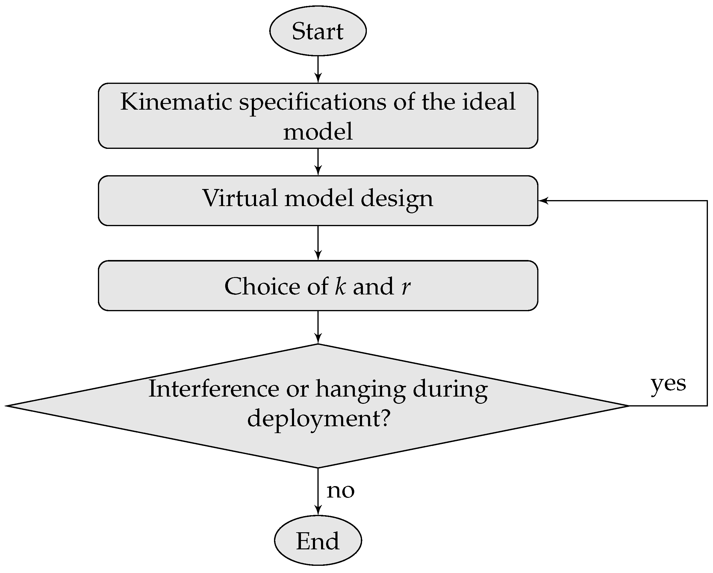
4.3. Spring-Damper System

The deployment mechanisms can be equipped with active systems [20,21], actuators, or passive spring-damper systems. Here, this third solution has been selected. Remarkably, the use of passive dampers or active vibration control is essential to dampen vibrations in orbit [22]. In order to avoid collisions, the angle between the two diagonal rods of a same cell in the folded configuration has been fixed equal to 3°. Consequently, the preload angle ${\theta }_0$ is equal to 177° while the preload torque is $C_p=k_m{\theta }_0$.

At this point, several simulations of the deployment phase have been carried out to find the spring stiffness and damping coefficient of the dampers, imposing an opening time of the mechanism of about 30 s as a constraint. The integration method and the values of the parameters used for the simulation have been adapted for the specific case of contacts as suggested in References [23,24,25,26]. The selection of the stiffnesses of the torsion springs was influenced by the maximum torsion angle, which must be greater than 177°, and by the diameter of the pin (8 mm) on which the spring is to be positioned. In particular, the following values were taken into consideration: 4.42, 5, 5.49, and 5.77 N·mm/deg.

Regarding the damping coefficient r of the dampers instead, the catalogs generally report the graphs of the damping torque as a function of the rotation speed, such as that of Figure 9. To derive the damping r, it has been considered that, in the case under examination, the mechanism must be unfolded within 30 s and that the springs are deformed by about 180°; therefore, the speed of rotation of the damper is of the order of 1 rpm. At these low rotational speeds, the linear relation $C_r=r\dot{\theta }$ is valid and the damping r therefore represents the slope of the initial linear segment of the curves in the Figure 9, which can be obtained as the ratio between the torque and the rotation speed set equal to 10 rpm. By interpolation on the ordinate axis and through appropriate conversions of the units of measurement, the values taken into consideration for the damping were: 20, 25, 35, and 40 N·mm·s/deg. Also in this case, the choice was influenced by the dimensions of the pin and the overall dimensions. The best combination of values, found after several simulations, turned out to be $k_m=5.77$ N·mm/deg and $r=35$ N·mm·s/deg. Indeed, this combination guarantees an acceptable opening time and, at the same time, it gives greater security regarding the correct deployment of the structure. Finally, in Figure 10, some frames of the dynamic simulation are reported related to the deployment phase with the selected stiffness and damping values, where the arrows in red represent the forces that vectors exchanged between the bodies in contact.

Figure 11, Figure 12 and Figure 13 respectively show the time evolution of the angle, angular velocity, and torque of the first spring-damper system. The results have been obtained considering the stiffness $k_m=5.77$ N·mm/deg and the damping coefficient r varying from 20 to 40 N·mm·s/deg. From Figure 11, it can be observed that, at time $t=0$ s, the angle is ${\theta }_0=177°$; moreover, the curves initially have zero slope, that is, zero angular velocity. Figure 12 confirms that the angular velocity is nonlinear with a higher velocity which decreases as the angle tends to zero, i.e., for the complete deployment of the opening mechanism. The deployment does not happen at a constant speed, but it happens at a higher speed at the beginning of the deployment phase and at slower speed at the end of this phase.

Figure 13 shows that the torque has an initial overshoot without subsequent oscillations, i.e., the system tends to the deployed configuration without oscillating. This trend is similar to that of an over-damped first-order system, that is with damping greater than the critical one; in fact, the function used by Adams for the torque calculation in the time domain is as follows:

$$C\left(t\right)=k_m({\theta }_0-\theta \left(t\right))-C_p-C_r\equiv -k_m\theta \left(t\right)-r\dot{\theta }$$

(6)

where $C_p$ is the preload torque and $C_r$ is the damping torque. The inertial term is ignored in the previous expression, as the structure must unfold very slowly in order to prevent unwanted vibrations. Thus, ignoring the inertial term, the second-order system is reduced to a first-order system.

It can be summarized that, with the increase of the damping coefficient r, the following occur:

• the curve of the opening angle becomes flat: the mechanism opens more slowly and therefore within a longer time,
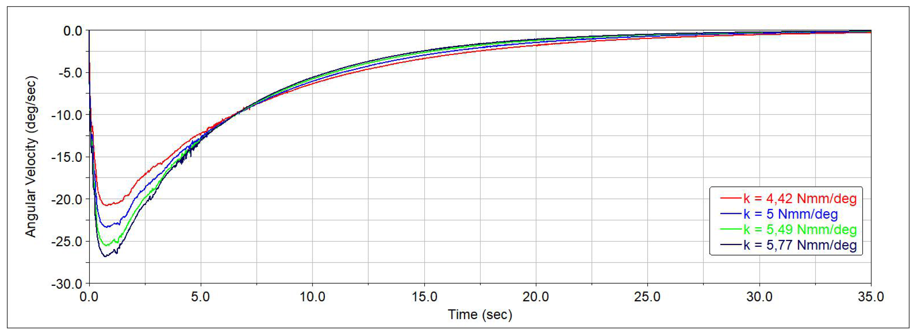
• the angular velocity decreases, and
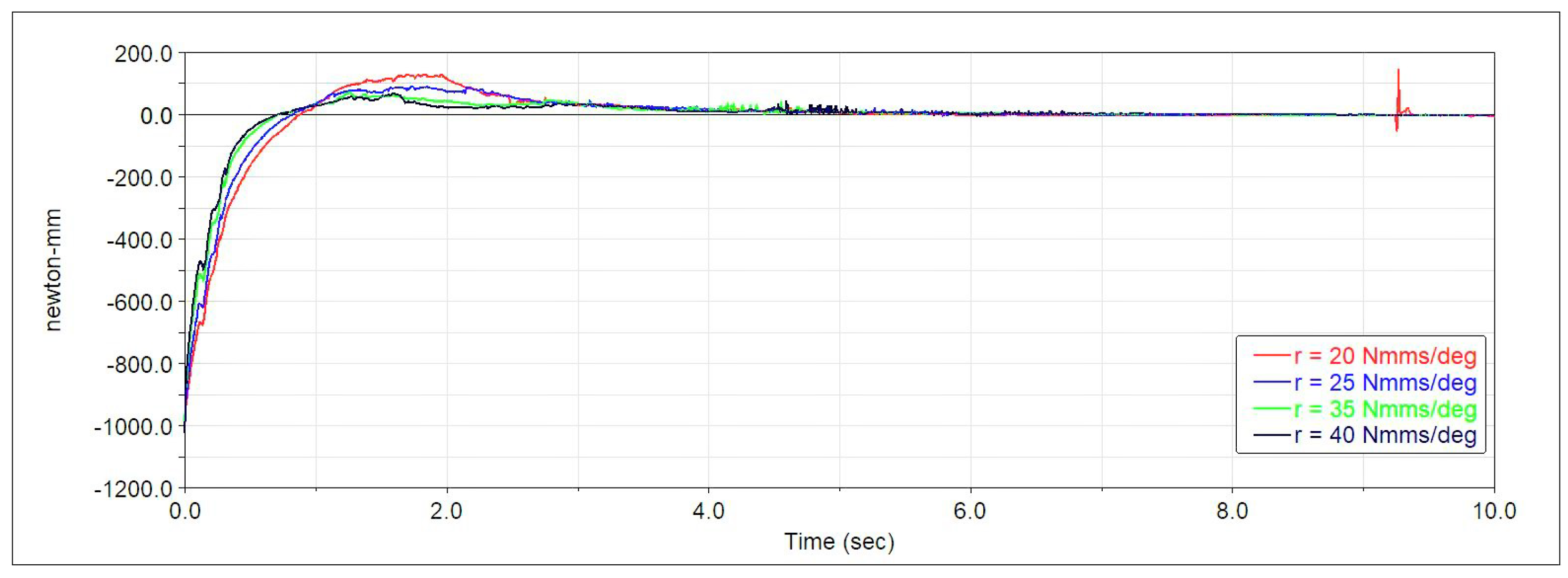
• the initial slope of the torque increases while the overshoot decreases.

Still referring to the first spring-damper system, Figure 14, Figure 15 and Figure 16 show the same plots obtained considering a fixed damping coefficient $r=35$ N·mm·s/deg and a variable stiffness $k_m$ in the range from 4.42 to 5.77 N·mm/deg. The curves differ slightly from each other due to similar stiffness values simulated. Increasing the stiffness $k_m$, the opposite behaviour with respect to the previous case is observed. As a matter of fact,

• the curve of the opening angle becomes sharp,
• the angular velocity increases, and
• the initial slope of the torque decreases while the overshoot increases.

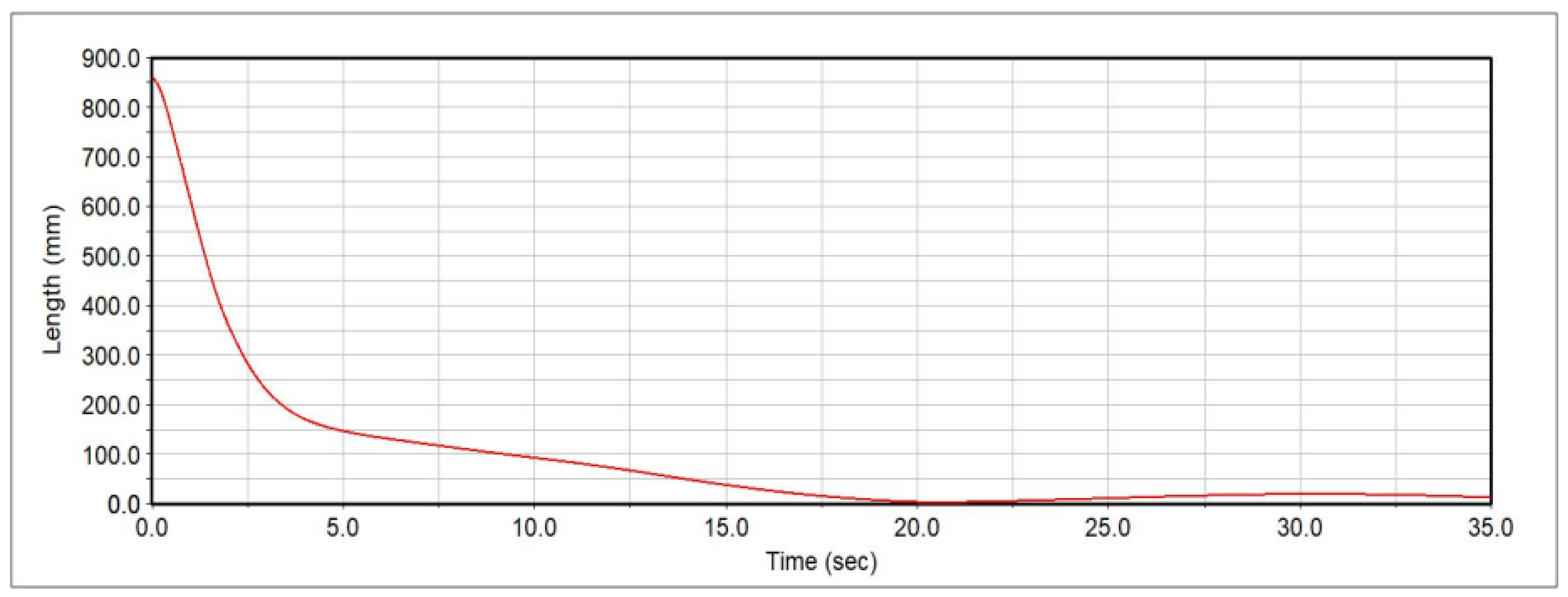
4.4. Deployment Time

The time needed to complete the deployment phase was determined using the Point-to-Point measure. In particular, we used the distance between the diagonal joint of the module 4 and the corresponding reference point relative to the structure completely deployed. During the simulation of the deployment phase, the measure in question decreases until it reaches the null value at the moment in which the full deployment occurs. In fact, Figure 17 shows the time-rate of the said distance measurement as a function of the simulation time. As noted in the previous subsection, there is a greater slope in the initial phase and a flat zone in the final phase. The full deployment of the mechanism takes about 24 s. The bounce appearing in Figure 17 is due to the clearance that has been introduced in all joints. When the distance measurement reaches the zero value, the latching mechanism is triggered. Due to the clearance, the mechanism bounces back and it settles down into a steady-state configuration very close to the ideal configuration, in which all the measurements should reach the zero value.

Varying the stiffness and damping coefficients using the same ranges provided in the previous subsection, we noted that, as the damping coefficient increases, the time required for the complete unfolding increases and, consequently, the deployment speed in the first phase of deployment decreases. Vice versa, as the stiffness increases, the time necessary for the full deployment decreases and, consequently, the deployment speed increases in the first deployment phase.

5. Conclusions

This paper has described the design of the opening mechanism of a LDR. An elementary cell has been chosen to assemble the octagon-shaped ideal kinematic model. The requirement on the diameter of the system has been defined considering the circle in which the octagon is inscribed. In order to avoid interference and encumbrances of the parts, the real design has been developed focusing on the joints. Three- and five-bar joints have been designed respecting joint functionality and ideal motions. The final design shows that the real system should be larger than the ideal system and that the ideal joint centers are found inside the real mechanism. By means of a numerical analysis and according to the different project parameters, it was possible to establish the dynamic behavior during the deployment phase, highlighting how the opening time varies by changing the stiffness and damping coefficients. Since the deployment phase takes place at low speed, the mechanism is not subject to excessive vibrations. Future developments include a finite element analysis with the corresponding calculation of the vibration modes. This will allow us to investigate how any unwanted vibrations can influence the deployment phase of the mechanism.

References

1. Freebury, G.E.; Beidleman, N.J. Deployable Reflector. U.S. Patent 10,256,530 B2, 9 April 2019. [Google Scholar]
2. Maddio, P.; Meschini, A.; Sinatra, R.; Cammarata, A. An optimized form-finding method of an asymmetric large deployable reflector. Eng. Struct. 2019, 181, 27–34. [Google Scholar] [CrossRef]
3. Henriksen, T.; Mangenot, C. Large deployable antennas. CEAS Space J. 2013, 5, 87–88. [Google Scholar] [CrossRef] [Green Version]
4. Freeland, R.; Bilyeu, G.; Veal, G.; Steiner, M.; Carson, D. Large inflatable deployable antenna flight experiment results. Acta Astronaut. 1997, 41, 267–277. [Google Scholar] [CrossRef]
5. Morterolle, S.; Maurin, B.; Quirant, J.; Dupuy, C. Numerical form-finding of geotensoid tension truss for mesh reflector. Acta Astronaut. 2012, 76, 154–163. [Google Scholar] [CrossRef] [Green Version]
6. Thomson, M. AstroMesh deployable reflectors for ku and ka band commercial satellites. In Proceedings of the 20th AIAA international communication satellite systems conference and exhibit, Montreal, QC, Canada, 12–15 May 2002. [Google Scholar]
7. Mobrem, M.; Kuehn, S.; Spier, C.; Slimko, E. Design and performance of astromesh reflector onboard soil moisture active passive spacecraft. In Proceedings of the 2012 IEEE Aerospace Conference, Big Sky, MT, USA, 3–10 March 2012. [Google Scholar]
8. Ryan, R. ADAMS—Multibody system analysis software. In Multibody Systems Handbook; Springer: Berlin/Heidelberg, Germany, 1990; pp. 361–402. [Google Scholar]
9. Pappalardo, C.M.; Guida, D. A time-domain system identification numerical procedure for obtaining linear dynamical models of multibody mechanical systems. Arch. Appl. Mech. 2018, 88, 1325–1347. [Google Scholar] [CrossRef]
10. Pappalardo, C.M. A natural absolute coordinate formulation for the kinematic and dynamic analysis of rigid multibody systems. Nonlinear Dyn. 2015, 81, 1841–1869. [Google Scholar] [CrossRef]
11. Cammarata, A. Optimized design of a large-workspace 2-DOF parallel robot for solar tracking systems. Mech. Mach. Theory 2015, 83, 175–186. [Google Scholar] [CrossRef]
12. Barbagallo, R.; Sequenzia, G.; Cammarata, A.; Oliveri, S. An integrated approach to design an innovative motorcycle rear suspension with eccentric mechanism. In Advances on Mechanics, Design Engineering and Manufacturing; Springer: New York, NY, USA, 2017; pp. 609–619. [Google Scholar]
13. Callegari, M.; Cammarata, A.; Gabrielli, A.; Sinatra, R. Kinematics and dynamics of a 3-CRU spherical parallel robot. In Proceedings of the ASME 2007 International Design Engineering Technical Conferences and Computers and Information in Engineering Conference, Las Vegas, NV, USA, 4–7 September 2007. [Google Scholar]
14. Cammarata, A.; Sinatra, R. On the elastostatics of spherical parallel machines with curved links. In Recent Advances in Mechanism Design for Robotics; Springer: New York, NY, USA, 2015; pp. 347–356. [Google Scholar]
15. Cammarata, A.; Caliò, I.; D’Urso, D.; Greco, A.; Lacagnina, M.; Fichera, G. Dynamic stiffness model of spherical parallel robots. J. Sound Vib. 2016, 384, 312–324. [Google Scholar] [CrossRef]
16. Villecco, F. On the evaluation of errors in the virtual design of mechanical systems. Machines 2018, 6, 36. [Google Scholar] [CrossRef] [Green Version]
17. Cammarata, A.; Lacagnina, M.; Sinatra, R. Closed-form solutions for the inverse kinematics of the Agile Eye with constraint errors on the revolute joint axes. In Proceedings of the 2016 IEEE/RSJ International Conference on Intelligent Robots and Systems, Daejeon, Korea, 9–14 October 2016. [Google Scholar]
18. Cammarata, A. A novel method to determine position and orientation errors in clearance-affected overconstrained mechanisms. Mech. Mach. Theory 2017, 118, 247–264. [Google Scholar] [CrossRef]
19. Giesbers, J. Contact Mechanics in MSC Adams-A technical evaluation of the contact models in multibody dynamics software MSC Adams. Bachelor’s Thesis, University of Twente, Enschede, The Netherlands, 2012. [Google Scholar]
20. Guida, D.; Pappalardo, C.M. Control design of an active suspension system for a quarter-car model with hysteresis. J. Vibr. Eng. Technol. 2015, 3, 277–299. [Google Scholar]
21. Pirrotta, S.; Sinatra, R.; Meschini, A. A novel simulation model for ring type ultrasonic motor. Meccanica 2007, 42, 127–139. [Google Scholar] [CrossRef]
22. Pappalardo, C.M.; Guida, D. Adjoint-based optimization procedure for active vibration control of nonlinear mechanical systems. J. Dyn. Syst. Meas. Contr. 2017, 139, 081010. [Google Scholar] [CrossRef]
23. Negrut, D.; Harris, B. ADAMS Theory in a Nutshell. Available online: https://www.me.ua.edu/me364/Student_Version/Digital_Appendix/adamsUofM.pdf (accessed on 13 February 2020).
24. Pappalardo, C.M.; Guida, D. System Identification Algorithm for Computing the Modal Parameters of Linear Mechanical Systems. Machines 2018, 6, 12. [Google Scholar] [CrossRef] [Green Version]
25. Cavacece, M.; Pennestri, E.; Sinatra, R. Experiences in teaching multibody dynamics. Multibody Sys. Dyn. 2005, 13, 363–369. [Google Scholar] [CrossRef] [Green Version]
26. Barbagallo, R.; Sequenzia, G.; Oliveri, S.; Cammarata, A. Dynamics of a high-performance motorcycle by an advanced multibody/control co-simulation. Proc. Inst. Mech. Eng. Part K J. Multibody Dyn. 2016, 230, 207–221. [Google Scholar] [CrossRef]
Figure 1. Elementary cells in fully and partially deployed configurations: (a) parallelogram with bar or diagonal cable; (b) pantograph; (c) v-folding rectangle; and (d) double vertical pantograph.
Machines 08 00007 g001
Figure 2. Deployment sequence of the proposed elementary cell.
Machines 08 00007 g002
Figure 3. Octagonal opening system and elementary cell.
Machines 08 00007 g003
Figure 4. Joints of the Large Deployable Reflectors (LDR) opening system.
Machines 08 00007 g004
Figure 5. Views of the proposed cell assembly.
Machines 08 00007 g005
Figure 6. Real LDR system.
Machines 08 00007 g006
Figure 7. Distance (mm) between the center of the joints in the ideal and real designs.
Machines 08 00007 g007
Figure 8. Phases of the mechanism design process.
Machines 08 00007 g008
Figure 9. Damping torque vs. rotation speed for different dampers present on the market (Catalogue ACE© Rotary Dampers FDT/FDN-47 to 70).
Machines 08 00007 g009
Figure 10. Some frames of the dynamic simulation of deployment of the real system, of which the sequence follows the alphabetical order.
Machines 08 00007 g010
Figure 11. Spring-damper system angle of the first cell as a function of the simulation time and when the damping coefficient of the damper varies from 20 to 40 N·mm·s/deg.
Machines 08 00007 g011
Figure 12. Spring-damper system time-rate angle of the first cell as a function of the simulation time and when the damping coefficient of the damper varies from 20 to 40 N·mm·s/deg.
Machines 08 00007 g012
Figure 13. Spring-damper system torque of the first cell as a function of the simulation time and when the damping coefficient of the damper varies from 20 to 40 N·mm·s/deg.
Machines 08 00007 g013
Figure 14. Spring-damper system angle of the first cell as a function of the simulation time and when the stiffness coefficient varies from 4.42 to 5.77 N·mm/deg.
Machines 08 00007 g014
Figure 15. Spring-damper system time-rate angle of the first cell as a function of the simulation time and when the stiffness coefficient varies from 4.42 to 5.77 N·mm/deg.
Machines 08 00007 g015
Figure 16. Spring-damper system torque of the first cell as a function of the simulation time and when the stiffness coefficient varies from 4.42 to 5.77 N·mm/deg.
Machines 08 00007 g016
Figure 17. Deployment of the LDR: Distance measurement vs. time.
Machines 08 00007 g017