1. Introduction
As crucial components in rotating machinery, bearings serve the primary function of transferring loads from moving machine parts to stationary ones, thereby facilitating the relative motion of the rotating components [
1,
2,
3,
4,
5]. The healthy operation of bearings is paramount for ensuring the safe production of rotating machinery. However, in most cases, bearings are subjected to prolonged exposure in high-speed, heavy-load, and corrosive environments, posing a substantial threat to the health of the bearings and leading to potential failures [
6]. Once a bearing fault occurs, it not only impacts the operation of the machinery itself but also exerts repercussions on subsequent production, triggering a chain reaction that can result in significant economic losses and even catastrophic accidents causing personnel casualties [
7,
8].
In recent years, with the rapid development of computer hardware technology, deep learning models have gradually become the mainstream method for bearing fault diagnosis due to their powerful feature extraction capabilities and end-to-end characteristics. Among them, convolutional neural networks [
9,
10], recurrent neural networks [
11,
12], and autoencoders [
13,
14] have received extensive attention from researchers. However, traditional deep-learning-based methods for bearing fault diagnosis still face certain challenges. Conventional deep learning models typically require a large amount of labeled data for training and assume that the training and testing data are under the same working conditions. In practical industrial production environments, however, the working conditions of rotating machinery (such as speed and load) may change with variations in work tasks, making it difficult to ensure that training and testing data are under identical conditions. Moreover, to prevent personnel injuries and potential damage to the machinery, equipment is promptly shut down once a fault occurs, making it impractical to collect a large amount of labeled data for each working condition [
15]. Therefore, achieving few-shot bearing fault diagnosis across different working conditions remains a challenge.
Currently, there are primarily three methods to address the aforementioned issues: data augmentation (DA), transfer learning (TL), and few-shot learning (FSL). DA involves enhancing the training data by applying diverse transformations and expansions to existing samples. Operations such as rotation, flipping, and scaling on images can generate additional training samples, thereby improving the model’s generalization capability. Jiang et al. [
16] proposed a novel generative adversarial-network-based ensemble data augmentation framework to address the issue of data imbalance in fault diagnosis. Wang et al. [
17] introduced a new compressed sensing data augmentation method for bearing fault diagnosis. While this method has achieved some success in mitigating sample scarcity, the introduction of excessive noise through data augmentation may result in disparities between generated samples and real samples. TL leverages knowledge acquired from one task to enhance performance on another related task. This approach facilitates the transfer of knowledge across different domains, allowing for the more efficient utilization of limited samples. Huang et al. [
18] proposed a deep adversarial capsule network designed for comprehensive fault diagnosis in industrial equipment. Zeng et al. [
19] introduced a transfer-learning-based fault diagnosis approach that integrates nearest neighbor feature constraints, specifically tailored for addressing cross-condition fault diagnosis challenges. However, if the differences between two domains are substantial, a model trained on the source domain may struggle to adapt well to the data distribution of the target domain. FSL is specifically designed to address problems with limited sample quantities. It involves designing more complex model architectures, utilizing advanced optimization algorithms, or incorporating prior knowledge, all aimed at achieving better performance under restricted data conditions. Wang et al. [
20] proposed a reinforced relation network for few-shot bearing fault diagnosis. Lei et al. [
21] introduced a novel prior knowledge-embedded meta-transfer learning approach to address the challenges of few-shot fault diagnosis under varying conditions.
In recent years, graph neural networks (GNNs) have begun to be employed in the field of few-shot fault diagnosis. Wang et al. [
22] propose a dual graph neural network to address fault diagnosis with limited data. Yang et al. [
23] propose a graph contrastive learning framework for few-shot machine fault diagnosis. GNNs are a type of deep learning model specifically designed for processing graph data. Graph data consist of nodes and edges, where nodes represent samples and edges signify relationships between nodes. Traditional bearing fault diagnosis methods primarily extract information from the amplitude of bearing vibration signals, overlooking the rich relational information among samples. Transforming vibration signals into graph data allows for modeling these relational details. The application of GNNs enables the deep exploration of relationships between nodes, aggregating this information to learn expressive node representations. Given that few-shot learning involves leveraging relationships between support set samples and query set samples for classification, GNNs exhibit significant potential in addressing few-shot classification challenges.
The main concept of GNNs is to learn expressive node representations through the propagation of information. However, the existing research [
24,
25] indicates that this propagation method encounters certain issues. Firstly, the majority of GNNs suffer from the problem of over-smoothing. As the network layers and iteration counts increase, the representations of all nodes tend to converge to a fixed point, rendering them independent of input features. Secondly, this propagation method makes each node highly dependent on its neighborhood, making nodes susceptible to potential data noise. Some approaches mitigate these issues through graph sparsification. Graph sparsification involves removing unnecessary edges in the graph to simplify its structure, enhancing model performance. Rong et al. [
26] alleviate over-smoothing by randomly dropping certain edges during training. However, random dropping may discard edges carrying essential information. Xiao et al. [
27] proposed an edge dropout threshold, removing edges with lower relevance in the graph to improve its quality. Yet, this threshold remains constant. Considering that the model faces varying difficulties in distinguishing different pairs of nodes, using a fixed threshold to determine whether to discard edges may impede the propagation of crucial information. Additionally, during the early stages of training, the model’s performance is suboptimal, and for pairs of nodes that are challenging to differentiate, the model may struggle to provide high similarity scores.
In response to the aforementioned issues, this paper proposes an adaptive dynamic threshold graph neural network (ADTGNN) for achieving cross-condition few-shot bearing fault diagnosis. The proposed adaptive threshold computation module (ATCM) in ADTGNN adaptively assigns thresholds to each edge. The threshold setting is related to the confidence of the edge, reflecting the model’s learning state regarding the nodes connected via the edge. This adaptive approach significantly reduces the risk of erroneously discarding edges carrying crucial information, greatly simplifying the graph and alleviating the over-smoothing issue. Additionally, we propose a dynamic threshold adjustment strategy (DTAS), where the constructed thresholds increase with the number of training iterations. This prevents the premature discarding of important edges during the early stages of training, thereby improving training speed and stability. The main contributions of this work are as follows:
To alleviate the over-smoothing issue in GNNs, an ATCM is proposed. This module adaptively sets thresholds based on the confidence level of edges, discarding edges with lower relevance and simplifying the structure of graph data.
A DTAS is proposed, where a relatively smaller threshold is assigned during the early stages of model training. With the increasing number of iterations, the threshold is gradually raised, preventing the premature discarding of important edges during the early stages of training.
An ADTGNN is proposed for cross-condition few-shot bearing fault diagnosis. By employing meta-learning strategies, the model rapidly achieves fault classification in the target working condition without the need for retraining, leveraging prior knowledge acquired from the known working condition.
The rest of the paper is organized as follows. In
Section 2 we present the details of the proposed method. In
Section 3, we validate the effectiveness of the proposed method on two public bearing datasets. In
Section 4, we summarize the work conducted.
2. Proposed Method
2.1. Problem Definition
The proposed method in this paper addresses the issue of cross-condition few-shot bearing fault diagnosis. Let denote the dataset composed of known working condition data, and denote the dataset composed of target working condition data. contains a large number of labeled samples, while has only a limited number of labeled samples. The proposed method requires training on to acquire prior knowledge and subsequently utilizes the small number of labeled samples from to classify unlabeled samples within . Specifically, we need to construct numerous few-shot classification tasks on . Each few-shot classification task consists of a support set (a set of a few labeled samples) and a query set (a set of unlabeled samples). If a support set has N categories, each with K samples, the few-shot classification task is referred to as an N-way K-shot classification task. The model needs to learn how to both utilize a small number of labeled samples for classifying unlabeled samples in these few-shot classification tasks and apply the learned experience to .
Figure 1 illustrates the workflow of the proposed ADTGNN for cross-condition few-shot bearing fault diagnosis. ADTGNN is primarily composed of four modules: the graph initialization module (GIM), the node feature update module (NFUM), the edge feature update module (EFUM), and the ATCM. The details of these four modules will be elaborated in the following subsections.
2.2. Graph Initialization Module
Let
represent an
N-way K-shot classification task, where S =
denotes the support set, Q =
represents the query set, and C is the number of samples in the query set. Here,
represents a sample. A convolutional neural network is employed to extract initial node features
from
, as shown in the following equation:
where
comprises two convolutional blocks and one fully connected layer. Each convolutional block includes a convolutional layer, BatchNorm layer, LeakyReLU activation function layer, and MaxPool layer.
represents the parameter set of
. To broaden the receptive field, a convolutional layer with a kernel size of 1 × 32 is applied in the first convolutional block. Let
denote the initial edge features, where
and
represent similarity and dissimilarity, respectively. The setting process for
is expressed as follows:
where
and
represent the labels of nodes
i and
j, respectively. Let
V =
denote the set of initial node features, and
denote the set of initial edge features. Based on
V and
, a fully connected graph
can be constructed and input into the following module for node feature updating and edge feature updating.
2.3. Node Feature Update Module
Based on the node features from the previous layer and the edges in the current layer, we can obtain the node features for the current layer, as shown below:
where
denotes the concatenation operation, and
represents the node feature updating network.
consists of two convolutional blocks, each comprising a convolutional layer, BatchNorm layer, LeakyReLU activation function layer, and dropout layer, and
is the parameter set of
. By setting a threshold for
and eliminating some edges, we can reduce the impact of redundant information during node feature updating. Additionally, during the update of
, both similarity-based aggregation information and dissimilarity-based aggregation information are considered, enhancing the expressive power of node features.
2.4. Edge Feature Update Module
Given the node features
and
at the
-th layer of the model, two metric networks,
and
, are employed to compute the similarity score
and dissimilarity score
. The process is outlined as follows:
where the network architecture of
is the same as that of
. Both consist of two convolutional blocks and a Sigmoid activation function layer.
and
are the parameter sets of
and
, respectively. Based on
and
, the current layer’s edge features
can be obtained through the following equations:
2.5. Adaptive Threshold Computation Module
For ideal node features, we desire their similarity to be significantly higher with nodes of the same class than with nodes of different classes. However, in reality, there are always some nodes that are challenging for the model to accurately cluster, especially during the early stages of training. The values of the edges depend on the nodes they connect, implying that for these challenging nodes, the network may struggle to compute edges with larger values. Therefore, when using a fixed threshold to remove unnecessary edges, there is a risk of erroneously discarding these edges, thus reducing the transmission of useful information in the graph. The goal of this paper is to adaptively set corresponding thresholds for each edge, thereby minimizing the risk of discarding useful edges erroneously. We design edge thresholds based on two principles. Firstly, the threshold setting should be related to the model’s confidence in the edges, reflecting the model’s learning state. Additionally, the confidence of edges should be related to the confidence of the nodes they connect.
For this purpose, before calculating the confidence of edges, it is necessary to obtain the confidence of the nodes. This paper utilizes the distribution features of nodes to measure their confidence. Given the distribution features of node
i as
, where
is composed of the similarity between node
i and the rest of the nodes. If the similarity of node
i with the nodes of the same class is significantly higher than its similarity with nodes of different classes, calculating the entropy of
will result in a smaller value. Conversely, if the similarity of node
i with nodes of the same class is not significantly higher than its similarity with the nodes of different classes, calculating the entropy of
will yield a larger value, as shown in
Figure 2.
Based on this principle, the confidence
of node i can be computed. First, utilize the following equation to calculate the entropy of
:
where
represents the uncertainty of node i. Let
, and normalize it to obtain
, as shown below:
represents the
i-th element of
. A higher value of
indicates that node
i is more challenging to distinguish, and its reliability is lower. The confidence
of node
i is then obtained using the following equation:
With the confidence of the nodes given, we can now calculate the confidence of the edge
, which depends on the confidences of nodes
i and
j:
Based on
, we can calculate the corresponding threshold
, and the process is as follows:
where
represents the global threshold, a constant. Since
,
will not exceed
.
changes with variations in
and
, enabling the adaptive adjustment of
based on
. The higher the value of
, the greater the model’s confidence in that edge, and
becomes closer to
.
2.6. Dynamic Adjustment Strategy of the Thresholds
During the early stages of training, the model’s performance is relatively poor, making it challenging to accurately determine similarity scores between nodes. In such cases, adopting a high global threshold may lead to the removal of some useful edges, causing instability in the training process. To address this, we establish a dynamic threshold
, which steadily increases with the number of network iterations
, preventing the premature discard of useful edges during the early training phase, as shown below:
where
is a constant.
Figure 3 illustrates the curve of
for different values of
. It can be observed that a smaller value of
leads to a smoother change in
. Due to the adaptive adjustment of
based on
and
,
will actually fluctuate and rise with the increase in
.
This paper aims to discard edges below a threshold through adaptive thresholding while leaving edges above the threshold unchanged. So, if the value of
is below
, we consider the relationship between these two nodes to be insignificant and set it to 0. Conversely, no action is taken. The equation is expressed as follows:
2.7. Label Prediction and Loss Function
Through L rounds of iterative updates, the
in the last layer of the network can serve as the final predicted edge label for the model. Let
, where
, represent the probability that nodes
i and
j belong to the same category. By utilizing the predicted edge labels between support set samples and query set samples, we can determine the predicted labels for the query set samples through weighted voting. Firstly, for node
i, we need to compute the probability
of it belonging to category
k, as shown below:
where
represents category
k. Subsequently, we can calculate the predicted label
for node
i using the following equation:
where
is a function that returns the index of the maximum value. Given the predicted labels and true labels for each layer of query set samples, ADTGNN is trained by minimizing the following loss function:
where
represents the set of true labels for the query set,
represents the set of predicted labels for the
l-th layer of the query set samples, and
denotes the binary cross-entropy loss function.
2.8. Fault Diagnosis Process
The fault diagnosis process of the proposed method is primarily divided into the following steps, as illustrated in
Figure 4:
Step 1: Initialize the network parameters of ADTGNN (, , , etc.).
Step 2: Given a dataset containing a large number of labeled samples under known working operating conditions, randomly select samples to form multiple few-shot classification tasks.
Step 3: Utilize ADTGNN to predict labels for the query set samples.
Step 4: Calculate the loss based on the predicted labels and true labels of the query set samples, and update the network parameters of ADTGNN using the gradient descent algorithm.
Step 5: If the training iterations reach the preset value, proceed to the next step; otherwise, repeat Steps 2 to 4.
Step 6: Employ the prior knowledge learned on to achieve fault diagnosis on the target working condition dataset , which contains only a small number of labeled samples.
3. Experimental Results and Analysis
To validate the effectiveness and to exhibit the superiority of the proposed ADTGNN, this paper conducted a series of comparison experiments using the Case Western Reserve University (CWRU) bearing dataset [
28], the Paderborn University (PU) bearing dataset [
29], and the drivetrain dynamics simulator (DDS) bearing dataset.
3.1. Dataset Introduction
The CWRU dataset is a publicly available dataset widely utilized in bearing fault diagnosis research, collected on the experimental platform illustrated in
Figure 5. It comprises vibration signals from motors working at 0 horsepower (hp) (1797 rpm), 1 hp (1772 rpm), 2 hp (1750 rpm), and 3 hp (1730 rpm). For each working condition, the dataset includes data from normal conditions (NCs), as well as various types of fault states. The fault types primarily consist of inner race faults (IFs), outer race faults (OFs), and rolling element faults (RFs). Electrical discharge machining is employed to simulate faults, with each fault induced by three different fault diameters: 0.007, 0.014, and 0.021 inches. This study conducts experiments using vibration signals collected from the drive end, with a sampling frequency of 12 kHz and a signal length of 1024 for each sample.
Table 1 provides a description of the working conditions used in this study.
The PU dataset is collected on a modular experimental platform, as illustrated in
Figure 6. This modular experimental platform consists of an electric motor, torque test shaft, rolling bearing test module, flywheel, and a load motor. By varying the speed of the drive system, the radial force on the bearing, and the load torque of the drive system, the PU dataset encompasses data from four working conditions.
Table 2 provides detailed information on the three working conditions used in this study. The detailed parameters of the faulty bearings used in this study are presented in
Table 3. The vibration signals used were measured via a piezoelectric accelerometer at the top adapter of the rolling bearing module, with a sampling frequency of 64 kHz and a signal length of 4096 for each sample.
The DDS dataset was collected on the drivetrain dynamics simulator of Spectra Quest, as illustrated in
Figure 7. Acceleration sensors were used at the parallel gearbox to gather vibration signals of five different types of bearings at motor frequencies of 15 Hz, 20 Hz, and 25 Hz. These types include NC, IF, OF, RF, and a combination fault (CF). The sampling frequency was set at 20 kHz, and the signal length for each sample was 2048.
Table 4 provides detailed information about the DDS dataset.
3.2. Experimental Setup
To validate the effectiveness of the proposed ADTGNN, this study constructed 18 cross-condition few-shot fault diagnosis tasks based on these three datasets. Each task requires the model to be trained on a known working condition dataset with a large number of labeled samples and tested on a target working dataset with only a few labeled samples. Five models were selected for comparison with the proposed ADTGNN: edge-labeling graph neural network (EGNN) [
30], prototypical network (PN) [
31], relation network (RN) [
32], DenseNet [
33], and ResNet [
34]. EGNN serves as the baseline model for the ADTGNN, and PN and RN have been widely used in recent years to address cross-condition few-shot fault diagnosis problems. DenseNet and ResNet are two popular deep-learning-based classifiers. Among them, PN, RN, EGNN, and ADTGNN use the same structure for feature extractors. The network parameters for the ADTGNN are specified in
Table 5. For the two parameters τ and δ in the ADTGNN, this study set them to 0.4 and 1.005, respectively.
The code used in this study is implemented on the Pytorch platform, employing the Adam optimizer with an initial learning rate of 0.0001. The meta-training and meta-testing rounds are set to 200 and 50, respectively. The computational platform used consists of an Intel (R) Xeon (R) Silver 4210 CPU at 2.20 GHz and an NVIDIA GeForce RTX 2080Ti GPU. To mitigate the impact of randomness, each experiment is repeated five times, and the results are averaged.
3.3. Analysis of Experimental Results on the CWRU Dataset
In order to better showcase the superiority of the proposed model, we introduced Gaussian white noise with a signal-tonoise ratio (SNR) of −6 dB into the original vibration signals from the CWRU dataset. The formula for calculating the SNR is as follows:
where
represents the power of the original signal, and
represents the power of the signal with added noise. As the intensity of the added noise increases, the SNR decreases. Taking the example of the inner race fault under 1 hp conditions,
Figure 8 illustrates the time-domain plots of the original vibration signal and the signal with added Gaussian white noise at −6 dB. It can be observed that after adding the noise, the fault features are obscured, significantly increasing the difficulty of fault diagnosis.
Table 6 and
Figure 9 display the experimental results of various models on the CWRU dataset. In
Table 6, A→B indicates that the model was trained on dataset A with a large number of labeled samples and tested on dataset B with only a few labeled samples. It can be seen that the accuracy of the proposed ADTGNN is consistently higher than that of other comparative models across six cross-condition fault diagnosis tasks. Under the 1-shot condition, ADTGNN achieves an average accuracy of 96.45%, surpassing EGNN by 2.83%. Under the 3-shot condition, ADTGNN demonstrates an average accuracy of 97.93%, exceeding EGNN by 2.26%. These findings highlight the superior performance of ADTGNN. From
Figure 9c, it can be observed that the average accuracy of various few-shot learning models under 3-shot conditions is higher than that under 1-shot conditions. This is well understood, as the more samples each class has, the more information the model can learn about that class. Under the 1-shot condition, the average accuracies of DenseNet and ResNet are significantly lower than the other four few-shot learning models. Especially in the C→A task, the accuracy of DenseNet is only 85.12%, and ResNet achieves an accuracy of only 85.41%. The reason for this may be that traditional deep learning training strategies hinder the models from acquiring better general experience, making it challenging to handle fault diagnosis tasks across different operating conditions.
3.4. Analysis of Experimental Results on the PU Dataset
Table 7 and
Figure 10 present the experimental results of various models on the PU dataset. It can be observed that under both 1-shot and 3-shot conditions, ADTGNN outperforms the other comparative models significantly. For instance, under the 1-shot condition, ADTGNN achieves accuracies of 97.01% and 97.51% in the D→E and F→E tasks, respectively, surpassing the second best by 2.47% and 6.08%. It is worth noting that under both 1-shot and 3-shot conditions, the average accuracy of PN and RN is lower than that of DenseNet and ResNeRN. The reason for this phenomenon may be that when there is a significant difference in the data distribution between the source and target domains, the relatively simple feature extractor structure of PN and RN prevents them from learning better general knowledge. From
Figure 10b and
Figure 10a, we observe that the performance of various models in the D→E and F→E tasks is lower compared to the other four tasks. For example, under the 1-shot condition, EGNN achieves 100% accuracy in the D→F task but only 94.54% and 91.43% accuracy in the D→E and F→E tasks, respectively. Referring to
Table 2, the probable reason for this is that changes in radial force have a significant impact on the probability distribution of bearing vibration signals. This leads to a substantial difference between known and target working condition data in the D→E and F→E tasks, resulting in poorer performance across all models. However, even under these conditions, the proposed ADTGNN outperforms the baseline EGNN, demonstrating the effectiveness of the improvements introduced in this paper.
3.5. Analysis of Experimental Results on the DDS Dataset
Table 8 and
Figure 11 display the experimental results of various models on the DDS dataset. It can be observed that under 1-shot and 3-shot conditions, the proposed ADTGNN outperforms the other comparison models across all six tasks. Under 1-shot conditions, ADTGNN achieves an average accuracy of 94.20% across the six tasks, which is 5.5% higher than EGNN. Under 3-shot conditions, ADTGNN achieves an average accuracy of 96.25%, surpassing EGNN by 4.02%. This can be attributed to the proposed ATCM and DTAS, which enable ADTGNN to adaptively set thresholds, thereby discarding some irrelevant edges and improving accuracy. From
Figure 11a, it can be observed that the performance of various models on the G→H and G→I tasks is relatively poor. The reason for this may be the significant distribution difference between dataset G and dataset H, resulting in the knowledge learned by the model in the source domain not effectively transferring to the target domain, especially in cases with small sample sizes. It is observed that under the 1-shot condition, the average accuracy of PN is only 82.03%, which is lower than DenseNet with 83.58% and ResNet with 84.47%. The potential reason for this could be that when there is only one sample per class, PN struggles to derive effective class prototypes, leading to relatively poorer performance. Moreover, ADTGNN maintains relatively high accuracy under the 1-shot condition. This is attributed to the transformation of one-dimensional vibration signals into a graph, enabling ADTGNN to effectively leverage relational information among samples during classification.
3.6. Analysis of Over-Smoothing Issue
Chen et al. [
35] proposed that the over-smoothing issue in GNNs may result from the excessive mixing of information and noise. In GNNs, interactions between nodes can bring useful information or irrelevant noise. For instance, interactions between nodes of the same class bring valuable information, making their representations closer to each other. Conversely, interactions between the nodes of different classes introduce noise, leading to learned representations that are indistinguishable. As the number of network layers increases, the acquired noise gradually outweighs the useful information, resulting in the over-smoothing problem. To validate the effectiveness of the proposed ATCM and DTAS in addressing over-smoothing issues, this study investigated the performance of EGNN and ADTGNN with different model layers in the challenging tasks of D→E and F→E. The experimental results under the 1-shot condition are presented in
Table 9 and
Figure 12.
It can be observed that for tasks D→E and F→E, when the model has two layers, both EGNN and ADTGNN achieve their highest accuracy. As the number of model layers increases, there is a varying degree of decrease in accuracy for EGNN and ADTGNN. However, compared to EGNN, ADTGNN exhibits a more gradual decline. For instance, in the D→E task, when the model has five layers, ADTGNN’s accuracy only decreases by 2.78% compared to its peak accuracy. In contrast, EGNN’s accuracy drops by 10.79%. This indicates that the proposed strategy in this paper effectively mitigates over-smoothing issues.
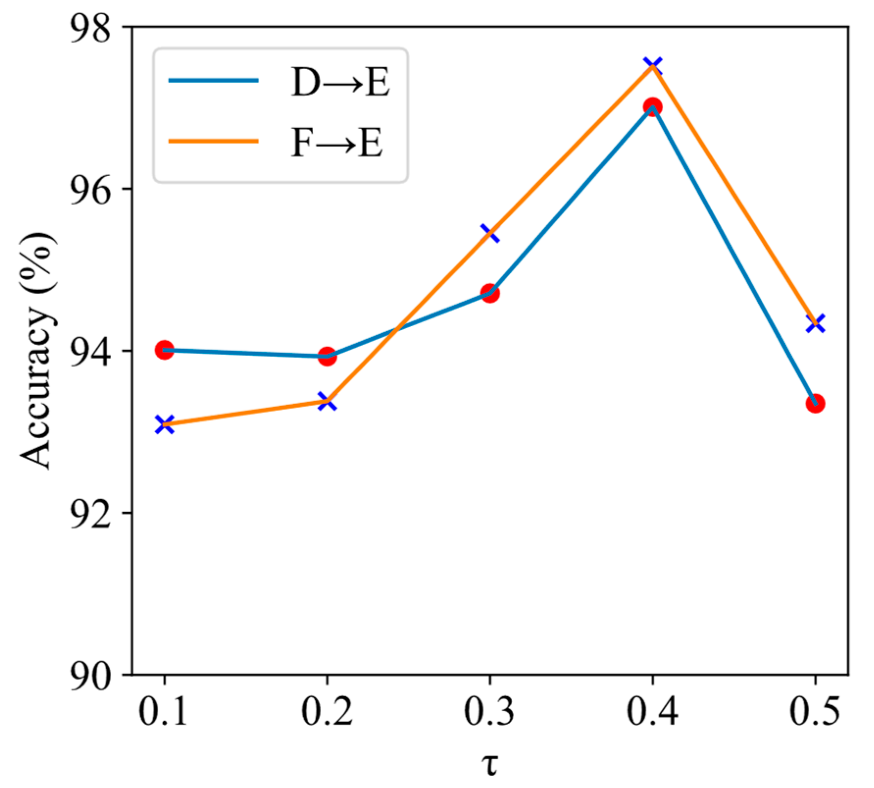
3.7. Selection of Parameter
In ADTGNN, a critical parameter, the global threshold
, has a substantial impact on the model’s performance. The choice of τ directly affects the upper limit of the adaptive threshold learned by the model. To explore the performance of ADTGNN under different τ values, we conducted experiments under the 1-shot condition, focusing on the challenging tasks of D→E and F→E. In these experiments, ADTGNN had a model depth of two layers, and the
value was set to 1.005. The results of the experiments are depicted in
Table 10 and
Figure 13.
It can be observed that ADTGNN performs best when . An excessively high may lead to the erroneous discarding of some useful edges, while an excessively low may result in the ineffective filtering of irrelevant edges.
3.8. Ablation Experiment
To assess the impact of the proposed ATCM and DTAS on the overall performance of the model, this study conducted ablation experiments on four challenging tasks. Here,
ADTGNN_1 indicates that the model does not use ATCM and DTAS. ADTGNN_2 indicates the model with a fixed threshold of 0.3 and without DTAS, while ADTGNN_3 indicates that the model only uses ATCM and not DTAS, with a τ value set to 0.4. The experimental results are presented in
Table 11. It can be observed that ADTGNN_3 exhibits significantly higher accuracy across all four tasks compared to ADTGNN_2. This is attributed to the proposed ATCM, which adaptively sets thresholds for each edge based on confidence, reducing the likelihood of erroneously discarding important edges. To demonstrate the effectiveness of DTAS more distinctly, this paper plotted the testing accuracy curves for ADTGNN_3 and ADTGNN in a specific experiment in
Figure 14. As seen in
Figure 14, ADTGNN achieves higher accuracy more rapidly than ADTGNN_3, particularly in tasks C→A and F→E. This is because during the early stages of training, the model’s performance may be insufficient, and setting high thresholds could result in erroneously discarding useful edges, leading to training instability. DTAS, by constructing dynamic thresholds, effectively enhances training stability. Finally, it can be observed that ADTGNN_1 exhibits the poorest performance among the four models. In summary, we can conclude that both the proposed ATCM and DTAS contribute to the overall performance of the model and are indispensable.
4. Conclusions
This paper proposes a novel cross-condition few-shot fault diagnosis method based on ADTGNN. ADTGNN is primarily composed of four modules: the GIM, the NFUM, the EFUMand the ATCM. Firstly, the one-dimensional vibration signal is transformed into a graph using the GIM. The graph is then input into the NFUM and the EFUM for feature transformation. The ATCM dynamically assigns thresholds to each edge based on its confidence, adapting and optimizing the graph structure, thereby effectively alleviating the over-smoothing issue in the graph. Furthermore, this paper proposed a DTAS, creating a dynamic threshold that gradually increases with the number of training iterations. This approach aims to prevent the model from prematurely discarding crucial edges in the early stages of training due to insufficient performance. Finally, fault diagnosis is achieved through a weighted voting mechanism. The proposed method’s superiority is validated through the construction of 18 cross-condition few-shot fault diagnosis tasks on three bearing datasets.
However, in order to achieve fault diagnosis across different working conditions, ADTGNN still relies on collecting a small number of labeled samples for each fault in advance. In future work, we will endeavor to address this issue.

 ,
, 


