Article

Multi-Rate Vibration Signal Analysis for Bearing Fault Detection in Induction Machines Using Supervised Learning Classifiers

by
Nada El Bouharrouti
1,*,
Daniel Morinigo-Sotelo
2 and
Anouar Belahcen
1
1
Department of Electrical Engineering and Automation, Aalto University, 00076 Espoo, Finland
2
Research Group ADIRE, ITAP Institute, Universidad de Valladolid, 47002 Valladolid, Spain
*
Author to whom correspondence should be addressed.
Machines 2024, 12(1), 17; https://doi.org/10.3390/machines12010017
Submission received: 8 November 2023 / Revised: 14 December 2023 / Accepted: 22 December 2023 / Published: 27 December 2023

Abstract

:
Vibration signals carry important information about the health state of a ball bearing and have proven their efficiency in training machine learning models for fault diagnosis. However, the sampling rate and frequency resolution of these acquired signals play a key role in the detection analysis. Industrial organizations often seek cost-effective and qualitative measurements, while reducing sensor resolution to optimize their resource allocation. This paper compares the performance of supervised learning classifiers for the fault detection of bearing faults in induction machines using vibration signals sampled at various frequencies. Three classes of algorithms are tested: linear models, tree-based models, and neural networks. These algorithms are trained and evaluated on vibration data collected experimentally and then downsampled to various intermediate levels of sampling, from 48 kHz to 1 kHz, using a fractional downsampling method. The study highlights the trade-off between fault detection accuracy and sampling frequency. It shows that, depending on the machine learning algorithm used, better training accuracies are not systematically achieved when training with vibration signals sampled at a relatively high frequency.

1. Introduction

Ball bearings are key components in rotatory machinery. They are widely used for their supportive role for rotating machine parts and transfer loads from one component to another. They allow lowering the frictional resistance between the machine components, leading to a globally higher mechanical efficiency [1]. As a consequence, ball bearings are subject to high preloading and stress during their lifetime [1,2]. This can lead to their failure and, hence, severe consequences for the machinery [1]. For electrical motors, it is estimated that between 40% [3] and 50% [4] of fault conditions are caused by bearing defects, depending on the application. For induction machines (IMs), bearing faults constitute a major issue [2,5], e.g., related to the lubrication of a bearing or fatigue in its mechanics [3]. In particular, for industry and companies, detecting a fault in a key component during continuous industrial operations and preventing it at an early stage are crucial steps to ensure the smooth functioning of industrial processes [6]. Nonetheless, bearing fault detection in an operating machine is challenging, particularly in the quest for cost efficiency. Therefore, condition monitoring (CM) has become essential to optimally detect and diagnose fault conditions in machinery such as IMs. By definition, CM relies on measurements and machinery parameters to make a diagnosis or prognosis about the health state of the machine [7]. More particularly, data-driven CM has become noteworthy for predicting failures before they occur, thanks to the development of artificial intelligence (AI) and classical statistical models [8,9]. Indeed, as explained by M. A. Khan et al. [9], traditional fault-detection methods like rule-based systems [10] and time-frequency analysis techniques [11] can face bottlenecks when dealing with larger or noisier datasets that require large computational efforts to process. In this sense, Zhang et al. [12] emphasized the great potential of AI for detangling complex patterns in diverse measurements, such as for vibration measurements.
The approach behind data-driven CM is illustrated in Figure 1 [8]. In the pre-operational phase, the purpose is to configure a machine learning (ML) algorithm able to identify patterns within the data about the health state of the machinery and recognize them in the operational phase. The algorithm thus relies on data to effectively learn how to diagnose and prognosticate a fault in practice [7]. These data which are related to the health state of the machinery are collected experimentally from a test-bench, e.g., as in [12,13], and/or via physical/mathematical simulations, e.g., as in [14,15]. As such, a dataset is formed with these data which then are preprocessed before being fed into a learning algorithm. During the preprocessing stage, the data are analyzed and organized to enhance their quality and make them suitable for effective ML model training. As such, an optimized learning process can start, where the ML model is trained on a share of the dataset, and then performances are evaluated on the rest of the dataset. The learning process is dynamic, as the algorithm’s training is continuously evaluated in tandem with the model’s performance during the evaluation phase. Once high evaluation performances are achieved, the model is used to handle operational tasks, where the ML algorithm analyzes and processes field operation data for CM purposes.
Recently, in data-driven CM using ML, many works have been developed for fault diagnosis and prognosis of ball bearings. Saberi et al. [16], Pandya et al. [17], and Rojas and Nandi [18] demonstrated the effectiveness of certain fault diagnosis schemes in the field of supervised ML, leveraging vibration signals for diagnostic purposes. Similarly, Qian et al. [19] and Kahr et al. [20] developed ML classifiers for bearing fault detection, using simulated vibration data to train these classifiers. More particularly, in ML, deep learning (DL) has also shown great potential for prognostics and health management in interpreting complex signals, such as vibrations [13,21]. In this sense, Kankar et al. [22] proved the effectiveness of using vibration signals to train an artificial neural network (ANN). Patil et al. [23] even assessed the quality of the wear of different ball bearing materials through ANN. Hotait et al. [24] proposed an ANN that aims at obtaining the degradation condition of rolling bearings for predictive maintenance. Brusa et al. [25] applied transfer learning to fined-tune pretrained models on audio-signals with vibration data relative to bearing faults, to detect faulty conditions. Considering all this, the approach of data-driven CM in the realm of AI is proven to allow for broader applications, thanks to the effectiveness of ML/DL algorithms in learning patterns and detecting anomalies in data over time. In industry, ML is increasingly perceived as a comprehensive solution for CM, reducing the need for manual feature extraction [21]; and as discussed by Park et al. [26], numerous modernized industrial operations aim to collect qualitative data related to training these AI algorithms. However, the cost of these measurements is related to their quality and their acquisition [27].
In the context of ball bearing fault diagnosis, vibrations are the most common signals used to train ML algorithms to detect ball bearing faults in IMs [9,28]. Experimentally, these vibrations are collected at a certain sampling frequency (SF) using accelerometers, often placed on the housing of the ball bearing in the IM [29]. A higher SF allows for finer precision in acquiring vibration data, but the price of these sensors also increases along with the SF [27]. As explained by Hadi et al. [6], the growing complexity of the data, e.g., implied by a higher SF while acquiring vibration data, makes the preprocessing of these data challenging (Figure 1). In addition, as highlighted by Rezaeianjouybari and Shang [13], the quality of a model is intricately tied to the quality of the training data. Therefore, as the SF of an accelerometer is a key parameter to the accuracy at which vibrations are measured, a trade-off should be aimed at between the computational efforts needed to process the data and the quality of the data.
In the literature, public datasets related to ball bearing vibrations under different health states have been acquired at SFs varying from 12 kHz to 64 kHz [12,30,31,32]. More precisely, the Case Western Reserve University (CWRU) bearing dataset [33] is widely used for detecting and diagnosing bearing faults in IMs. In this dataset, vibrations were collected using accelerometers attached to the housing of ball bearings at SFs of 12 kHz and 48 kHz in steady-state operations. This is acknowledged as a standard reference for validating models [12,14,34]. In practice, its usage also allows studying the diagnosis of a wide range of applications, e.g., as shown by Liu et al. [35], who introduced a fault diagnosis method for wind turbine fan bearings using the CWRU dataset. Many reviews examining AI-related techniques for fault diagnosis employing this dataset have been conducted, e.g., in [34,36,37], and have proven its efficiency in the fields of ML and DL [12,13,38,39,40,41].
While numerous studies have showcased successful fault detection techniques employing ML on the CWRU dataset, only a few papers have addressed the issue of the dataset’s quality in contrast with the performance of ML algorithms. Most papers concentrated on the quality of the fault diagnosis scheme itself, as exemplified in [42] for the time-frequency ridge approach or in [11] for improving a time-frequency methodology, rather than on the quality of the data themselves. On this latter topic, in the literature, AlShalalfeh and Shalalfeh [43] studied the diagnosis of bearing faults under data quality issues for the CWRU datasets and showed that lower SF measurements hinder good diagnosis of bearing faults through AI. Nevertheless, no extensive study has addressed the topic of the SFs at which the vibration data are acquired and their impact on the performances of AI-related fault diagnosis schemes for data-driven CM. This topic deserves more attention when one thinks of the computational and economical costs involved in the processing and storing of large and precise data [6,13]. Therefore, instead of focusing on the fault diagnosis scheme itself, the present research work proposes to understand if acquiring vibrations at lower SFs can be efficient enough to train robust ML algorithms for fault detection.
In this paper, several AI algorithms for fault classification were trained and evaluated on vibration signals sampled at different rates to detect bearing faults using the CWRU dataset. The performance of these algorithms was evaluated with respect to the signal sampling rates (SRs), i.e., their SFs. This way of proceeding relates to the quality requirement relative to the data one should aim at in order to build a robust AI classifier for fault diagnosis. As such, this paper starts by presenting a multi-rate sampling methodology, which aims to acquire signals at various SRs, utilizing an experimental signal collected at a high SF from the CWRU bearing dataset. Then, AI-based methodologies employed for the classification of these signals are introduced mathematically. The following sections present an analysis of the classifier training and evaluation performance for each SR according to three paradigms. To conclude, a discussion of the findings is presented.

2. Multi-Rate Sampling Methodology

This section introduces the multi-rate sampling methodology applied to the vibration data, which inherently consists of time series. It starts by explaining the concept of fractional resampling and then elaborates on how resampling a signal influences a ML algorithm. The multi-rate sampling method presented here is primarily based on the work of de Jesus Romero-Troncoso [44].

2.1. Fractional Resampling

Fractional resampling is a method used to adapt the SR of digital signals to a desired target SR [44]. In this paper, fractional resampling was performed to process digital signals collected from accelerometers placed on an IM initially acquired at a specific source SR and subsequently resampled using non-integer scaling factors. Fractional resampling was performed according to [44], as follows:
  • STEP 1—Upsampling through Interpolation: The first step in fractional resampling consists in interpolating the signal. An interpolation of rate q consists in a multi-rate signal process, which generates interpolated samples between two original signals [44]. Therefore, due to the interpolation of q times, the SF f s becomes a resampled S F   f r , according to
    f r = q f s
    This step is important in fractional sampling, because it effectively increases the source SR, without acquiring additional physical samples. In other words, by generating interpolated samples between the existing ones, one can obtain a higher temporal resolution of the signal, which is particularly valuable when dealing with signals that change rapidly over time, similarly to vibrations. As a result of (1), as the S F increases, the data sequence is similarly increased by a factor q of the interpolation rate.
  • STEP 2—Low-Pass Filter (LPF): By interpolating a signal, spectral distortion can be introduced due to the underlying mathematical principles and limitations of the interpolation process, e.g., due to signal aliasing or simply the time variation in the signal. This distortion can result in the introduction of quantization noise into the interpolated signal [44]. As a consequence, introducing a LPF is important to deal with such interpolation effects and reduce spectral distortion. The LPF has a cut off frequency, f c u t o f f , respecting
    f c u t o f f = S F 2
  • STEP 3—Downsampling by Decimation: Decimating a digital signal consists of the opposite of interpolating it. Through the decimation process, the number of samples in the original signal is reduced by a factor p, and the S F   f s is modified due to the decimation [44], as follows:
    f r = f s p .
    By definition, the decimation step acts as a LPF because it reduces the number of samples and deletes the high-frequency bands of the original signal. However, similarly to the length modification of the signal after interpolation, the length of the original sequence after decimation is decreased by a factor p.
Interpolation and decimating procedures can be combined into a multi-rate fractional resampling technique, which is obtained as the result of these three steps (Figure 2). At the end of the procedure, the resulting SR is f r expressed as [44]:
f r = f s q p .
In addition to this, the frequency resolution becomes
Δ f r = f s N q p .
where N is the length of the digital signals.
Figure 2. Fractional resampling steps of a digital signal x ( n ) ; x ( r ) is the interpolated sequence after the application of a LPF; x ( s ) is the decimated sequence of x ( r ) [44].
Machines 12 00017 g002

2.2. Multi-Fractional Resampling in Machine Learning

ML classifiers require a large amount of qualitative data points in order to be well trained and perform during on-site applications [12,13]. Vibration signals are long time-series of data whose length N is determined by their S R as follows:
N = S R × T t o t
where T t o t is the signal duration [s]. Therefore, when decimating a signal, as its S R is reduced according to (3) and needs to adhere to the Nyquist theorem to avoid aliasing, the number of samples in the decimated signal is effectively reduced. More precisely, high-frequency components are cut after fractional resampling if the new SR is lower than the initial SR [44]. This reduces the signal length and the number of samples available to train the ML algorithms. However, higher frequency components are often associated with noise and removing them might be beneficial to the training of the ML algorithm. Therefore, while canceling these noisy high frequency components, ML algorithms might suffer from a lack of data to properly learn the intrinsic patterns in a dataset [13] and a trade-off should be sought between noise cancellation and the number of samples available.
Additionally, the type of ML classifier used is a crucial choice for any dataset, and consequently, a balance must be maintained between resampling and algorithm performance. Therefore, in research work like the present one, where vibration data are resampled, it is important to provide a comprehensive examination of a wide range of ML algorithms and how they may suffer or benefit from data resampling.

3. Machine Learning Classifiers

In this section, three different classes of ML classifier are introduced along with their mathematical formulations: linear classifiers, tree-based methods, and neural networks. For each of the techniques presented, it is also explained how these classifiers apply to vibration signals.

3.1. Linear Classifier

A linear classifier is a type of supervised ML algorithm that divides a dataset into multiple classes by finding a linear decision boundary between them. This decision boundary is represented as a hyperplane in the feature space, which separates data points belonging to the different classes. Linear maps in the context of ML linear classifiers are essentially the weight vectors and bias terms used to make predictions based on input features. In the case of linear classifiers, the hyperplane is defined by the following linear map [45]:
h w : R n R , x w T x .
The function h w linearly maps the n-dimensional feature vector x R n × 1 through the weight vector w R n × 1 to the predicted label [45]. In this, n corresponds to the number of features in the input vector x . More generally, in the hypothesis space H ( n ) R n , each particular linear hypothesis h w belongs to this space through
H ( n ) : = { h w : R n R , h w ( x ) : = w T x } .
H ( n ) is the set of all possible linear maps from R to R n . Each linear hypothesis represents a specific machine learning linear classification method. For a binary problem, the classification is performed on either side of the linear predictor map h w for a certain parameter vector w . For multi-class classification, hyperplanes are added and therefore create subsections in the classification. In the present study, two linear methods were chosen: support vector machines (SVM) and multinominal logistic regression (MNLR). They have proven their good performance in the diagnosis of bearing faults [16,17,18,46].

3.1.1. SVM

SVM is a linear classifier that draws a hyperplane in an n-dimensional feature space so that the margin between the classification groups is maximized. By definition, the optimal hyperplane between classes is the one that maximizes the distance between the adjacent points of these classes [16]. For each observation i, the boundary line is defined as follows [16]:
y i ( w · x i + b ) 1 , for i 1 : k
y i j = 1 n w j · x i , j + b 1 , for i 1 : k
with x i R n × 1 being the feature vector of the i-th sample whose element x i , j R represents the j-th feature of the i-th sample, w R n × 1 the weight vector that defines the orientation of the hyperplane whose element w j R represents the weight of the j-th feature, b the bias term R which shifts the hyperplane, y i R the class labels of the samples the boundary as the SVM classifier, and k the number of samples. In order to define the optimal boundary, the distance between the x i and the boundary needs to be calculated. This is expressed as [16]:
r = y i ( w · x i + b ) | w |
Using the condition in (9), the hyperplane is determined through optimizing (11) and, thus, solving the following:
minimize w , b 1 2 | w | 2 .
When the dataset is not linear and noisy, e.g., as for vibrations, relaxed constraints might be added to the optimization (12), to allow the classification to adjust to this non-linearity [16]. These relaxed constraints are brought by introducing slack variables ξ i as
minimize w , b 1 2 | w | 2 + C i = 1 N ξ i .
ξ i R 0 measures the classification error for each point i; C R + is the slack penalty, which aims at maximizing the margin and minimizing the training error. These new constraints are subject to a new boundary lines equation, defined as
y i ( w · x i + b ) 1 ξ i .
These equations are solved with Lagrangian multipliers and dual decomposition [16]. As far as vibration signals are concerned, the SVM using (14) is more suitable for a classification based on vibration signals due to their significant temporal variability.

3.1.2. MNLR

MNLR is a linear classifier that extends the concept of logistic regression for multi-class classification problems. By definition, logistic regression is a binary classification method for feature vectors x R n × 1 , which have a binary labeling. They are linear models in the sense that the relationship between the i-th component x i of feature vector x , and the logarithmic probability of an event occurring is modeled as linear [45]:
log P ( y = 1 ) 1 P ( y = 1 ) = β 0 + β 1 x 1 + β 2 x 2 + + β k x k , for i 1 : k
where β k R are the coefficients of the model, y R is the corresponding label, and P ( . ) R is the probability of an event occurring. After the prediction of the label of each feature vector x , a loss function is computed to quantify the error between the predicted value and the actual label. As far as logistic regressions are concerned, the cross-entropy loss has to be minimized to minimize the discrepancy between the predicted probabilities and the actual binary outcomes:
Cross Entropy Loss = y log ( p ) + ( 1 y ) log ( 1 p )
where p R is the predicted probability that the feature vectors belong to class 1.
Based on this, MNLR enlarges the concept of logistic regression to multiple class classification by reusing the concept of cross-entropy loss but changing the predicted probability distribution. The workflow of the MNLR is constituted by three layers, including a linear model, but also by introducing a softmax layer for the multidimensionality of the data labels, before calculating the cross-entropy [46]. The softmax function transforms a vector of k real numbers into a probability distribution over k possible outcomes and, by consequence, introduces multi-dimensionality. This makes the method suitable for the classification of non-linear datasets, such as for vibration data. The softmax equation is
s o f t m a x ( x ) i = e x i j = 1 k e x j , for i 1 : k .
The softmax function takes an input vector x R k where x i represents the i-th element of x , exponentiates each element x i , and divides it by the sum of the exponentiated values of all elements in the input vector. The predicted label y ^ R of the feature vector x is thus obtained as follows:
y ^ = s o f t m a x ( x · w ) + b

3.2. Tree-Based Methods

A tree-based ML method for classification is a type of algorithm similar to a hierarchical structure composed of nodes and branches, where each node represents a decision based on a feature, and each leaf node represents a class label of these features. More practically, a decision tree is a step-by-step multi-classification, which computes the function h : X Y and maps the features x X to their predicted labels h ( x ) Y [45]. The objective function for a decision tree with maximum depth k is given by
Objective ( T ) = i = 1 N L ( y i , y i ^ ) + α · f ( k ) .
In this equation, Objective ( T ) is the objective function to be minimized for a certain decision tree model T, N is the number of training samples, L ( y i , y i ^ ) is the loss function for the i th sample, α R is a regularization parameter, f ( k ) R is a function of the tree complexity based on the maximum depth, y i R is the true label for the i th sample, and y ^ i R is the predicted label for the i th sample. The goal is to find a decision tree that minimizes this objective function, balancing the fit to the data with the complexity of the tree.
As far as the classification of vibration signals is concerned, tree methods are interesting for supervised ML because the number of health states is predetermined by the data labels, which refer to the tree depth straightforwardly. However, vibrations acquired at a low SF can have a limited amount of data points after post-processing, in addition to a non-linear and noisy nature. In these cases, gradient-tree-boosting methods are used as they enhance the capabilities of tree models, making them particularly useful when dealing with limited data points obtained from vibrations acquired at a low SF [28,47]. In the context of boosted trees, the objective function aims to build a model of sequential decision trees. Each new tree is fitted to the negative gradient of the loss function with respect to the current model’s predictions. This process minimizes the following objective function:
Objective ( F ) = i = 1 N L ( y i , F ( x i ) ) + m = 1 M Ω ( T m ) .
Objective ( F ) is the objective function of the predictive function F to be minimized, N is the number of training samples, L ( y i , F ( x i ) ) is the loss function for the ith sample with respect to the current model’s predictions, M is the number of trees in the ensemble, T m and Ω ( T m ) are respectively the mth decision tree in the ensemble and its regularization term. This regularization term controls the complexity of the individual trees, to prevent overfitting. Common gradient boosting algorithms used for fault diagnosis of ball bearings based on vibration signals include XGBoost [48] and LightGBM [49], each with their own variations on the objective function and optimization techniques.
In particular, XGBoost, which stands for extreme gradient boosting, is an enhanced tree-based ML method that extends traditional gradient boosting techniques. It sequentially builds decision trees and minimizes a combined objective function that balances model accuracy and complexity. The hierarchical structure of the traditional decision trees in a gradient boosting approach is mathematically expressed through the minimization of an objective function, as seen in (19), where the objective is to find a series of decision trees that collectively minimize the combined loss, to improve predictive accuracy. As such, XGBoost can process complex and non-linear signals such as vibration signals, and it has widely proven its efficiency in data-driven CM using the CWRU dataset, e.g., in [48,50]. Therefore, in the present paper, XGBoost was chosen as the illustrative tree-boosting ML method to be compared with the other ML algorithms studied in this research work.

3.3. Neural Networks

Neural networks consist of interconnected artificial neurons that mimic the structure of the human brain, allowing them to process vast amounts of data and perform complex tasks efficiently [45]. For vibration signals, ANNs are able to discern patterns within each time series, even in the presence of significant noise in the measurements, as they learn the inherent patterns of the data. ANNs are composed of several layers of neurons, and the operation of a neuron is mathematically the following:
  • Weighted Sum: Each input x j R is assigned a weight w i , j R . Hence, the i-th neuron computes z i R as the addition of a weighted sum and a bias term b i R , as
    z i = j w i , j x j + b i .
  • Activation Function: After computing z i R , the neuron applies an activation function σ ( z i ) that introduces non-linearity into the neuron’s response according to
    σ ( z i ) = σ j w i , j x j + b i
    The choice of the activation function is particularly important in the context of a study about vibrations, because it introduces non-linearities and enables the effective capture of dynamic and time-varying behaviors.
A condensed notation to express the operation of an entire layer of m neurons is the following:
σ ( z ) = σ W T x + b
where W R n × m is the weight matrix, x is the n-dimensional feature vector, b is the m-dimensional bias vector.
In the present work, two types of ANN are used, i.e., a multilayer perceptron (MLP) and recurrent neural networks (RNNs). They are used as they provide a lot of flexibility and have proven their efficiency within the framework of bearing fault detection, as in [51,52]. The main difference between the two is that an MLP is a feedforward ANN, while an RNN incorporates recurrent connections that enable information to persist over time steps. As such, the effect of the network architecture on the model’s ability to capture temporal dependencies and sequential patterns in the data was studied, along with the quality of the vibration signals.

3.3.1. MLP

An MLP is an ANN whose architecture has multiple hidden layers of feedforward neurons, which are the intermediary layers between the input and output of the MLP. The idea is similar to a simple linear classifier improved using activation functions and with several layers interconnected. In the context of multi-class classification, given a dataset with N samples and K classes, the MLP predicts an output p R K × 1 from an input vector x R n × 1 as follows: first, it applies (23) in every layer of its architecture, and then uses a softmax operation, as in (17), on the output of its last layer. In this case, the output p = [ p 1 , , p K ] is a vector whose entries p j ( j 1 : K ) are the estimated probability of the corresponding classes.
The objective function for a MLP in multi-class classification is the categorical cross-entropy loss computed as
Categorical Cross Entropy Loss = 1 N i = 1 N k = 1 K y i , k · log ( p i , k ) .
y i , k R is equal to one if the true class label for sample i is k, or zero otherwise. p i , k R is the predicted probability of sample i belonging to class k according to the MLP’s output. The goal during training is to minimize this loss by adjusting the weights and biases of the MLP using optimization algorithms. In the context of vibrations, the MLP classifies different time series based on the input features to a specific vibration pattern according to the MLP’s output, by minimizing the loss in (24).
While MLPs capture complex patterns in static data, they often face difficulties when dealing with time-dependent data, such as vibration. In an MLP, each input x is processed independently without any consideration of its temporal relationship with other inputs. Importantly, there is no mechanism for the MLP to consider the history of previous inputs when computing the current output y , as indicated by (23). This lack of memory is a fundamental limitation as it prevents considering the time-dependency of each datapoint in a time series, where understanding the temporal context is crucial. By introducing recurrent connections into their architecture, RNNs address this issue.

3.3.2. RNN

An RNN is an ANN which allows neurons to maintain memory and consider past inputs by introducing feedback loops between the neurons. It makes them more suitable for sequential time-dependent data, while tackling the limitations of the feedforward architecture typified by MLP. The equations for an RNN can be expressed as follows:
  • Hidden State Update: For a layer with m neurons, taking an input x t R n × 1 at time t, the hidden state update is defined as
    h t = σ ( W h h h t 1 + W x h x t + b h ) .
    h t R m × 1 represents the hidden state at time t, σ is the activation function, W h h R m × m and W x h R m × n are weight matrices for recurrent and input connections, and b h R m × 1 is the bias vector;
  • Output Computation: At every time t, for a K-class classification task, the output y t R K × 1 is computed from the hidden state as follows:
    y t = σ ( W h y h t + b y ) .
    In this equation, W h y R K × m is the weight matrix connecting the hidden state to the output, and b y R K × 1 is the output bias. Compared to (23), the output is now a function of the weight matrices for the input and output connections, as shown in (25);
  • Categorical Cross-Entropy Loss to Minimize for Classification: Similarly to the MLP, the cross-entropy loss as defined in (24) is an objective function which is then minimized during training.
These steps show how an RNN processes sequential data with feedback between neurons, allowing it to model temporal dependencies. In the present paper, a specific type of RNN is considered, long short-term memory network (LSTM). A LSTM network provides a mechanism for maintaining short-term memory in the RNN by optimizing the retention of important context and dependencies over a substantial number of timesteps. It has demonstrated its efficacy in classifying vibration data for bearing fault diagnosis [52]. LSTM thus provides an interesting foundation to study the impact of data quality on an ANN, considering its performance with respect to MLP, i.e., an analysis of architectures of ANNs with and without recurrent connections.

4. Methodology

In this section, the implementation of the methodology used to configure the previously presented ML classifiers with signals sampled at different SF is presented, as well as the extraction and pre-processing of these same data.

4.1. Numerical Experimentation Flowchart
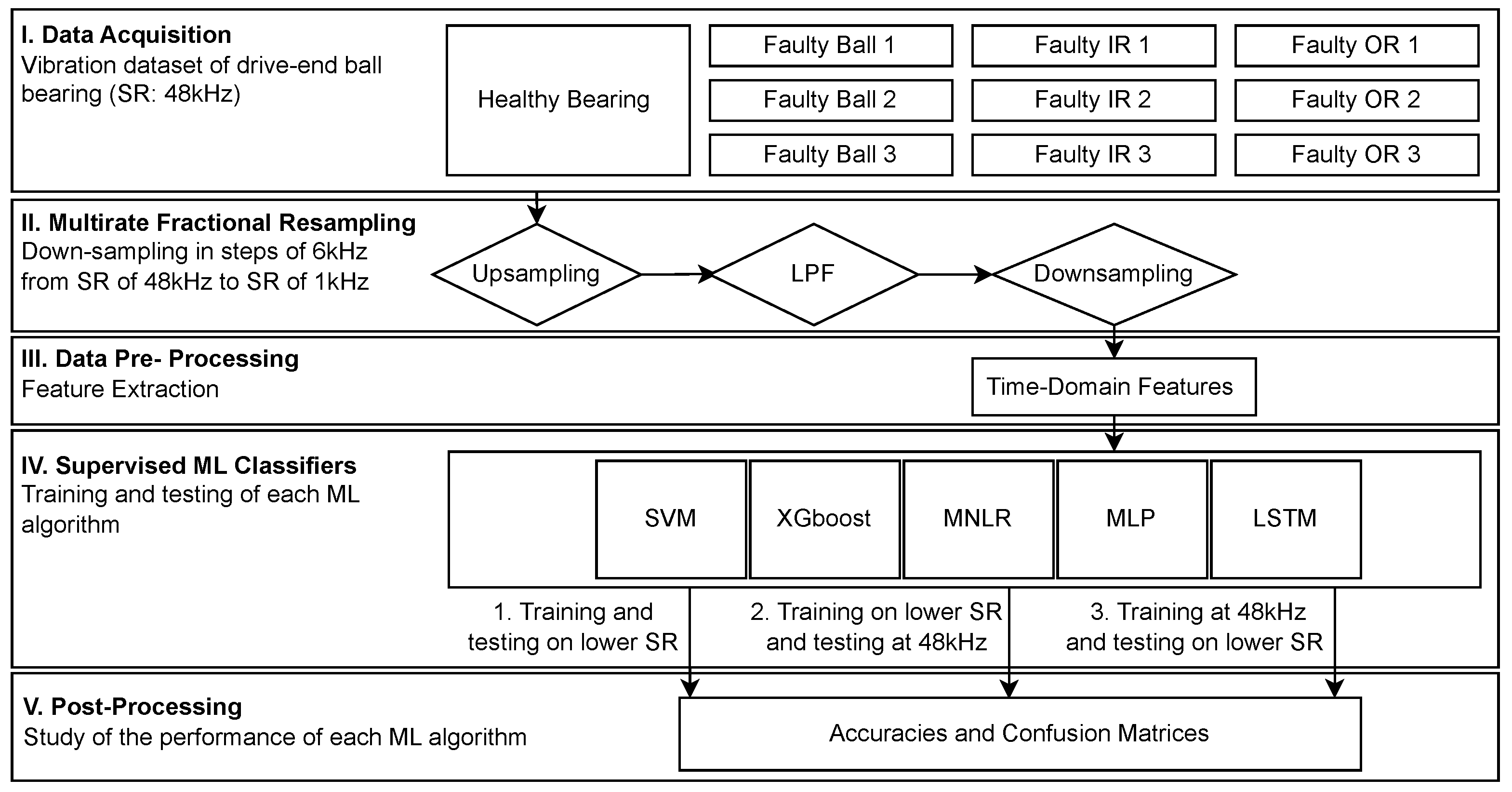
The methodology used to study the effect of the SF of vibration signals on the performance of ML algorithms is described in Figure 3. It is organized in five steps.
I.
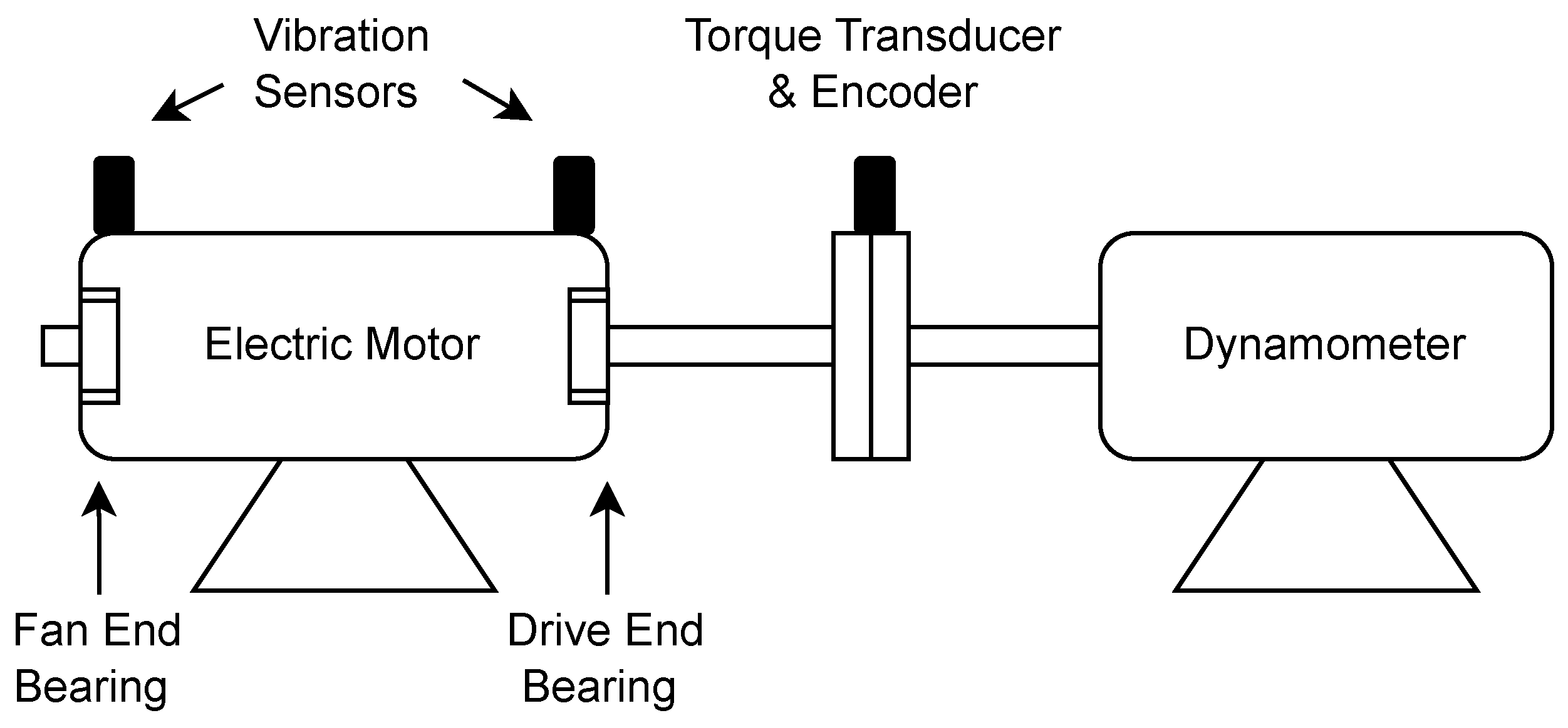
Data Acquisition: Experimental data about vibration signals related to ball bearing faults in an IM acquired at a SF of 48 kHz were obtained from an the CWRU dataset [33] detailed in Section 4.2;
II.
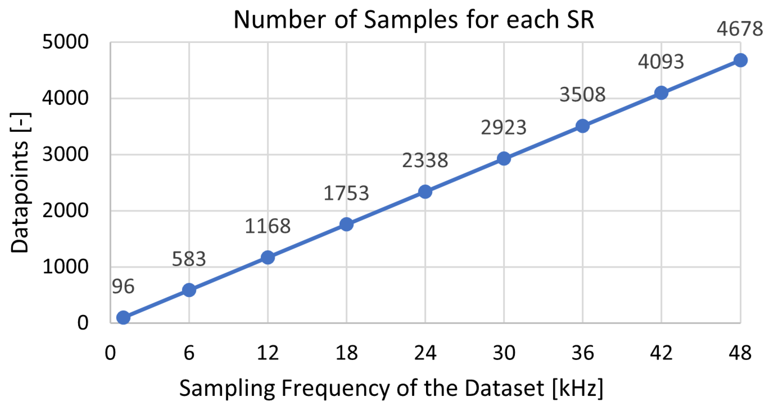
Multirate Fractional Resampling: Each vibration signal for each bearing state (faulty ball, faulty inner ring (IR), faulty outer ring (OR), healthy bearing) was resampled using a step of 6 kHz from the initial SR, i.e., 48 kHz. Therefore, vibration signals for each of the time-series were downsampled to 1 kHz, 6 kHz, 12 kHz, 18 kHz, 24 kHz, 30 kHz, 36 kHz, and 42 kHz. The design choice of resampling the signals by a step of 6 kHz was driven by the fact that, in the literature, most datasets of bearing vibration acquired their signals at a SF which was multiple of 6 or relatively close to it, e.g., 12, 20, or 48 kHz [12,33]. It was thus concluded that 6 was a good metric to cover a large number of SRs, while remaining close to actual figures.
Afterward, the downsampled signals were studied separately in the following steps;
III.
Data Pre-processing: The downsampled signals for each respective SR were then preprocessed and time-domain features were calculated as a preparation for the training and evaluation of the ML algorithms;
IV.
Supervised ML classifiers: Supervised ML classifiers were trained and tested based on data from the different time-series previously generated. These classifiers learned and accurately recognized patterns within the features extracted from the vibration signals. Three scenarios were studied:
  • The objective was to train the ML classifiers to detect various bearing faults for each SR and to test the performance of the classifiers at the respective SR. By doing so, the ML algorithm’s ability to classify at low(er) SR was studied, i.e., under varying data acquisition conditions;
  • This step was similar to the first one but tested the performance of the classifiers on the initial data sampled at 48 kHz. By doing so, the robustness of the ML classifiers was evaluated, as they were tested on finer data;
  • Vice-versa, this step trained the ML classifiers on the initial data sampled at 48 kHz and evaluated the algorithms on vibration signals sampled at a lower SF.
V.
Post-Processing: The accuracy of each ML algorithm was evaluated for both training and testing according to the metric previously described in Section 3. Afterwards, the length of the downsampled signals, i.e., the number of data-points after feature extraction, was calculated for each SF and evaluated, to observe the correlation with the performance of the algorithms.
As far as the software used for the implementation of the method is concerned, the points I., II. and III. in Figure 3 were implemented on Matlab R2023b. For points IV. and V. in Figure 3, the ML classifiers were trained and evaluated on Python. This choice was made as the respective software have libraries and pre-installed functions relative to the data resampling and ML, i.e., sci-kit learn (sklearn), SciPy, keras, tensorflow for Python, and specifically the resample() function on Matlab, which proved its efficiency in resampling vibrations, as explained in Section 5.1.
As the methodology developed in this work has been introduced, the CWRU test-bench used to collect the experimental measurements and the data acquisition process are now presented.

4.2. Experimental Set-Up and Data Acquisition

The dataset used consisted in several time-series of vibration signals obtained from a test-bench of the CWRU [33]. The set up consisted of an electric motor, a dynanometer, a torque transducer with encoder, and an electric motor where two bearings were placed to support the motor shaft, i.e., an SKF 6205-2RS JEM ball bearing at the motor drive end and an SKF 6203-2RS JEM at the motor fan end.
Both bearings were tested with localized faults, i.e., artificial faults caused through electrical discharge machining. More specifically, the faulty balls (rolling element), IR faults, and OR faults were used under working conditions from 0 W, 745.7 W, 1491.4 W, and 2237.1 W (corresponding to 0 to 3 HP in [33]) motor powers with shaft speeds of 181.1, 183.4, 185.7, and 187.8 rad/s (corresponding to 1730, 1750, 1772, and 1797 rpm in [33]). Vibrations were measured in normal and faulty conditions thanks to vibration sensors, i.e., accelerometers, placed on the motor housing (see Figure 4). Each measurement lasted 10 s and was acquired at SRs of 12 kHz and 48 kHz. The vibrations were collected using a 16-channel DAT recorder, which were then processed into Matlab files (.mat) provided in [33].
In the present work, the dataset was constructed with ten different bearing conditions, as shown in Table 1. In total, the dataset included ten health states of the bearing, from normal (healthy) bearing conditions to the different faulty cases implemented at a loading level of 735.5 W, i.e., 1 HP in [33], and at a speed of 187.5 rad/s, i.e., 1772 RPM in [33]. To ensure signal synchronization, the vibration signals of the ten health states were adjusted to the minimum size signal, corresponding to 381,888 samples per signal. The signals were also normalized to a similar scale, to avoid later bias in the ML algorithms and enhance the convergence of the latter.

4.3. Dataset Pre-Processing

In ML, feature extraction is an important step before training any algorithm, to be able to extract essential information from complex datasets. It allows the identification of key patterns, like anomalies or outliers, within the signals. Thanks to this process, the dataset is simplified, making it more suitable for classification tasks. Extracting features in the data aims at forming a dataset of pertinent features, while optimizing the size of the dataset but also enhances the efficiency of the classification procedure. In this research, twenty time-domain features were selected according to [16] (see Table 2). It is to be noted that frequency-domain features were discarded for the present study, as time-domain features showed high performing results in the ML classification, using the experimental dataset provided. In addition to this, choosing not to use frequency-domain features prevented the use of extensively working in the frequency domain while performing downsampling, because downsampling techniques can introduce spectral deformation and leakages in the Fourier transformation [44]. Therefore, the present study was limited to time-domain features to effectively study the effects of different sampling rates on the ML classifiers.
For every vibration signal, the twenty time-domain features were computed individually. This calculation was performed in sequential batches, where each batch was subjected to the computation of the corresponding twenty time-domain features through a specified procedure. Balancing computational efficiency, memory conservation, and adaptability to different signal characteristics, the length of each batch was determined as a fraction of the overall signal size using a deliberately chosen factor of 234, including a 50% overlap between consecutive batches. This deliberate choice was carefully studied and was chosen to ensure continuity and coherence during this research study. Afterward, for every signal, the number of batches was calculated by rounding the division of the signal length by the batch-size obtained to the nearest integer. As such, each resampled vibration signal was systematically divided into manageable batches, while taking into account the desired degree of overlap.

5. Results

In this section, the results of the downsampling of the vibration signals are explained, as well as the results of the effects of the downsampling on the ML algorithms previously introduced.

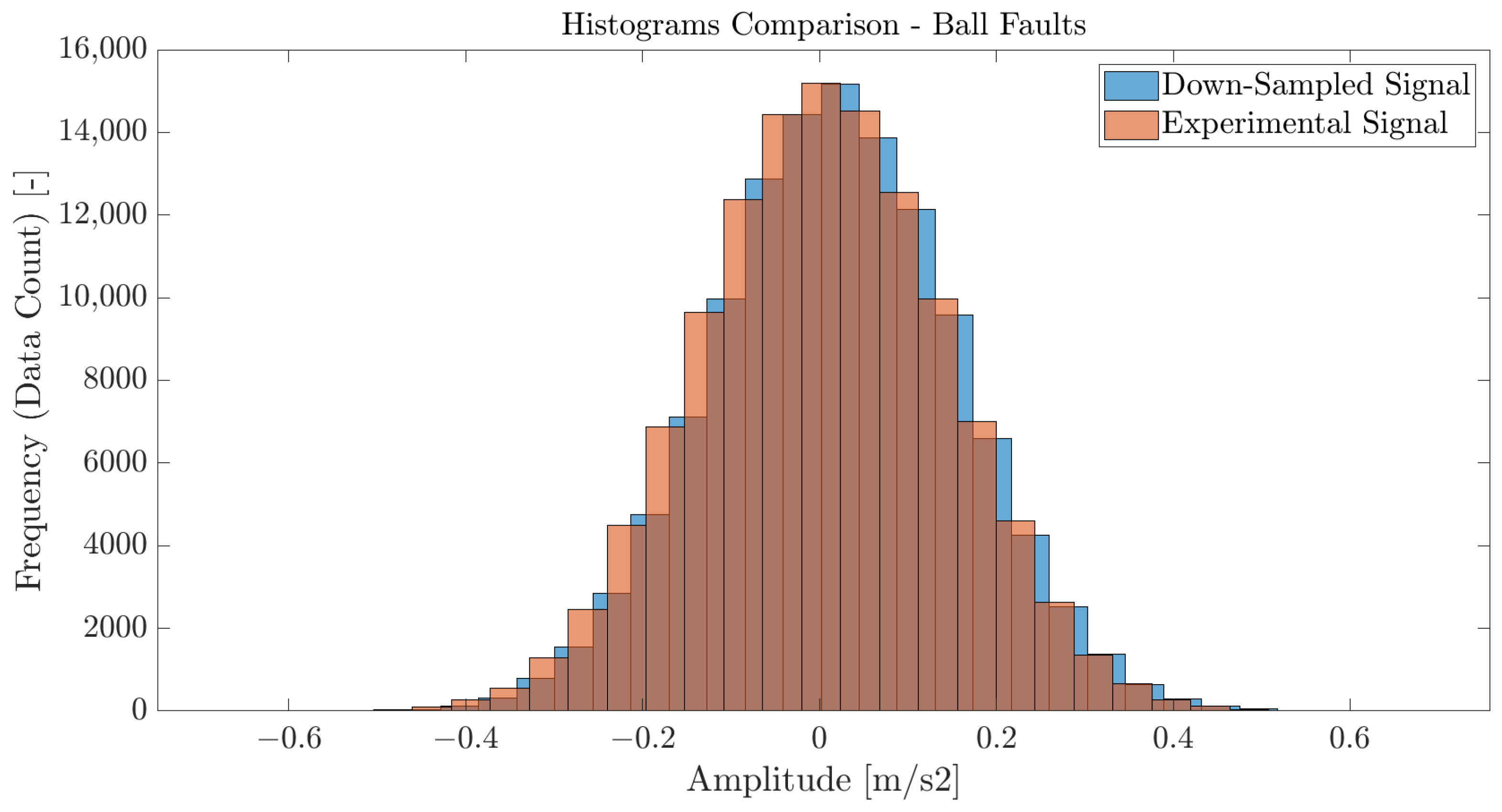
5.1. Evaluation and Verification of the Downsampling Method

The fractional resampling was performed using the integrated function of Matlab resample(x,p,q,n) which resamples the input time-series x, as the ratio p q of the original SR of x, through decimation and interpolation (see Figure 2), using Chebyshev anti-aliasing LPF of order 2 × n × max(p,q). For each fractional resampling, the integration and decimating parameters p and q were chosen such that the radio p q was an irreducible fraction.
In [33], the CWRU datasets contain vibration signals measured at two sampling rates: 12 kHz and 48 kHz. In the present work, the vibration signals acquired at a SR of 48 kHz were downsampled to 12 kHz and compared to the experimental measurements acquired at 12 kHz. This way of proceeding allowed verifying the approach of downsampling and its accuracy. This analysis was conducted for all faulty conditions, expect the healthy bearing conditions, as the CWRU dataset does not provide measurements under a healthy bearing condition at a SR of 12 kHz. In this section, the analysis of the downsampling method is shown for the vibration signal of a bearing having a 0.178 mm ball fault. This experimental comparison provides a consistent verification for other types of vibration signals, i.e., other IR, OR, and ball fault severities.
In order to quantify the difference between the experimental and downsampled signals of 12 kHz SR, it is worthwhile to study statistical features, as done in [53]:
Kurtosis = 1 N i = 1 N x i x ¯ σ 4 .
Variance = 1 N i = 1 N ( x i x ¯ ) 2 .
Skewness = 1 N i = 1 N x i x ¯ σ 3 .
Energy = i = 1 N ( x i ) 2 .
x ¯ is the mean of the signal x, σ x is its standard deviation, x ¯ is the mean of the experimental signal, and N is the number of datapoints. These quantities were chosen to evaluate the quality of the downsampled signals, as they are statistical features relaying on the quality of the probability distribution of the signals. For each of the signals, the kurtosis, variance, skewness, and energy are displayed in Table 3.
For each signal feature, a comparative interpretation is given.
  • Kurtosis: The kurtosis of a signal measures the sharpness of the peaks in a probability distribution; i.e., how often outliers stand in the signal. In the present case, the kurtosis values for both scenarios were close, with a difference of 0.05, which means that the tails of the two scenarios were fairly similar, yet slightly more pronounced in the downsampled signal;
  • Variance: The variance of a signal measures the spread of data points in a signal with respect to the mean value of this same signal. Here, the two cases share similar variance values, meaning that the dispersion of the data was consistent between the downsampled and experimental signals;
  • Skewness: The skewness measures the asymmetry of a probability distribution. In the two scenarios studied here, the skewness was very low, suggesting that the distributions were rather symmetrical, with a tendency towards positive skewness;
  • Energy: The energy is a measure of the total signal power. Here, the downsampled signal had a higher overall power compared to the experimental signal, but the values in the two cases only had a difference of 0.66%.
In addition to the signal features, histograms of the two signals have been plotted in Figure 5. Histograms are visual representations of the distribution of data values within a signal [54] and they allow the assessment of the signal’s central tendency, spread, and shape. In addition to that, histograms provide insight into the presence of outliers or unusual data points. In this case, the two analyzed vibration signals displayed nearly identical histogram distributions, with a slight x-axis shift, reflecting minor differences in data point distribution across vibration amplitudes and synchronization. However, the number of samples remained consistently similar in both signals, highlighting their strong correspondence in underlying data patterns.
Therefore, based on the signal features and the histograms analysis, it can be concluded that the downsampling procedure of vibration signals was experimentally verified for 12 kHz and could be generalized to other levels of resampling with the same method. As such, the study of the effect of the SF on the ML algorithms could be pursued.

5.2. ML Classifiers Performance

In this section, the training and testing performance of the ML classifiers on the multi-rate vibration signals is detailed for the three scenarios described in the methodology, Section 4.1.

5.2.1. Training and Evaluation at Respective SRs

Before delving into the results, it is crucial to elucidate the rationale behind the selection of the hyperparameters used for tuning the five ML algorithms. These hyperparameters were primarily chosen based on established practices found in the literature, such as [55,56]. However, they were also assessed through a firsthand experience of the authors with fault diagnosis schemes using AI, particularly with the scikit-learn library in Python. Consequently, SVM used the radial basis function, i.e., rbf, as kernel; the MNLR made use of ‘lbfgs’ solver, with a maximum iteration limit of 1000 chosen arbitrarily as trade-off between the computational efficiency and convergence of the algorithm. XGBoost was configured with parameters tailored for multi-class classification, i.e., “multi:softmax” objective function related to the softmax transformation and the log-likelihood loss [47]. Using Keras and Tensorflow, the MLP and LSTM architectures had two hidden layers, excluding input and output layers, which respectively comprised 128 and 64 layers each employing the rectified linear unit, i.e., ReLU, activation function [56]. Both employed an ADAM optimizer for optimization with cross-entropy loss. The batch size was set at 32 and the number of epochs at 50 epochs for MLP and LSTM algorithms. It is to be noted that a study about the influence of the epochs on the training and validation accuracies of the two ANN was also conducted. Throughout the three experiments, the data were scaled and the hyperparameters remained unchanged in the three scenarios. The accuracy metric was consistently used for the model evaluation.
Moreover, prior to presenting the results, it is also essential to describe the dataset used and how the training and evaluation datasets were formed. As a result of the preprocessing of the data described in Section 4.3, the dataset with vibrations sampled at 48 kHz contained 4678 samples, from which 80% were used for training and 20% for evaluation. As a consequence, for the same share of the data between training and evaluation, after pre-processing the data for the feature extractions, the signals sampled at 1 kHz contained much less data for training than the higher SR signals (Figure 6). One can easily perceive this in (6).
The training and evaluation accuracies for each signal for their respective SR are shown in Figure 7. In this case, the ML algorithms trained with signals sampled at a certain SF were also evaluated for the classification task of vibration signals sampled at the respective SFs.
Based on the results, an improvement in the accuracies was globally observed for signals sampled at higher frequencies, particularly for signals whose SR equaled or was higher than 12 kHz. However, training performances after this SF did not improve. Instead, there was rather a small drop in the training performances for higher SFs or, at most, a stagnant behavior. This observation shows that algorithms trained on vibrations acquired at a higher SF do not systematically imply better training, even if a higher SF allows for finer measurements. Particularly, a higher SF might involve the acquisition of more complex and noisier signals, which challenge the ML-algorithms in their performances. Each of the ML algorithms exhibited distinct characteristics in its behavior:
  • SVM and MNLR: The linear classifiers were able to classify bearing faults but showed a lower performance for signals sampled at 1 and 6 kHz. This means that for these SRs, these algorithms did not learn from the training dataset in order to define the decision boundaries between the classes;
  • XGBoost: XGBoost, as a tree based model, is the ML algorithm which was the least sensitive to the downsampling of the vibration data. Indeed, the training accuracy remained at its maximum value, despite the change in SR. It was able to learn well from lower sampled datasets, while maintaining a high performance. Based on theory (Section 3.2), the training procedure in XGBoost is inherently robust to variations in dataset size and distribution. It uses an ensemble of decision trees with features like gradient boosting and regularization, which allows it to adapt effectively to different data representations, ensuring a stable performance, even with a reduced sample density. During the evaluation, the highest performance of XGBoost was achieved at 24 kHz. This did not seem to imply anything or result from any specific feature of the dataset at this SF, especially as the evaluation performance remained in the same range as the other performances obtained, i.e., above 90% accuracy;
  • MLP and LSTM: As neural networks, MLP and LSTM are by definition more sensitive to the amount of samples [12,13]. The low SR lost fine-grained information about the health conditions of the bearing, which made it harder for these neural networks to learn patterns and achieve high performances. However, due to its architecture, LSTM can capture longer-term dependencies in sequential data and this provides some advantages in scenarios with limited data. Therefore, at a SR of 6 kHz, LSTM was already catching up with performance of the other ML algorithms and even surpassed the linear models. As far as the MLP is concerned, it seemed to globally lag behind compared to the other ML algorithms, no matter the SR. At a lower SR, MLP suffered from lack of qualitative information to learn correctly, but at high-frequency, MLP might not have been able to generalize higher dimensional spaces as well.
It is to be noted that the ML algorithm performances became roughly equivalent for data whose SR was above 18 kHz. Excepting the extreme stability of XGBoost, the training accuracy of the other ML algorithms seemed to slightly decrease above this value. This might have been due to the fact that a higher SR allows capturing more noise in the dataset and more peculiar phenomena, which might have complicated the pattern identification within the dataset.
As a trial to improve the performances of the neural networks for signals sampled at 1 kHz, the number of epochs during training was increased, while analyzing their respective performances. By definition, the number of epochs refers to the number of times the entire training dataset is passed forward and backward through an ANN during the training process [57]. Therefore, increasing the number of epochs in MLP and LSTM can potentially improve accuracy, particularly when the dataset is limited, as this enhances the training length. The results are shown in Figure 8.
As the number of epochs increased, the performance of the models globally increased. The models found more opportunities to learn, perceive the variations in the dataset, and adjust their weights accordingly, thus improving their performances during training and evaluation, while reducing their underfitting in the case of a lack of qualitative data. However, the number of epochs studied was high and the performances increased unstably, which might indicate overfitting, in addition to the fact that the evaluation accuracy was higher than the training accuracy above 350 epochs. Indeed, the models became too specific to the training set, and for a small dataset such as the one of 1 kHz, it was harder to strike a fair share of training and evaluation data, as there were fewer datapoints for the model to learn from and evaluate (see Figure 6).

5.2.2. Training at Lower SRs and Evaluation at 48 kHz

As a second part of the study, training was performed as for the previous section but now the evaluation was carried out on a dataset of signals acquired at a SR of 48 kHz. This way of proceeding assessed the robustness of the models trained at lower sampling rates and their ability to generalize to higher-frequency data. The results are gathered in Figure 9.
As shown, the ML models trained on signals with an SR equal or higher than 12 kHz performed well but MLP lagged behind, with an accuracy of 70% at this SR. However, from 30 kHz, it was able to catch up with the performances of the other ML algorithms, with an evaluation accuracy above 80%. This means that, in general, the ML models trained on signals sampled with an SR equal or higher than 12 kHz identified the patterns of the healthy and faulty conditions of the ball bearing well enough that they could classify complex and noisy signals sampled at 48 kHz case. Reducing the SF of a signal inevitably diminishes its resolution according to (5). Consequently, when ML algorithms are trained on signals sampled at lower SF, where finer details are less distinguishable, they may struggle to accurately recognize nuances and intricacies introduced by the higher SF. Conversely, as explained in Section 5.2.1, when these same algorithms are trained on a highly sampled signal, they might lack information from the evaluation set sampled at a lower frequency to recognize the very-detailed explanations they have been trained on. This interplay between the SF and the training set’s resolution highlights the importance of carefully considering signal characteristics in the development and evaluation of ML algorithms.
Additionally, as for the previous study, one can see that XGBoost remains the leading ML algorithm for such an application. Therefore, a confusion matrices for each test was plot in Figure 10, Figure 11, Figure 12 and Figure 13 to demonstrate that the improvement in the classification for the dataset with vibrations sampled at 48 kHz gradually increased along with the SR of the vibrations of the training sets. Based on these figures, it does not seem that there was any specific tendency for some faults to be classified better at a lower sampling rate. Therefore, only a generic increase in the classification improvement was concluded.
While the confusion matrices demonstrated a generic enhancement in classification, it is crucial to acknowledge that this improvement lacks empirical validation. Specifically, upon comparing Figure 11 and Figure 12, certain samples from signals recorded at 48 kHz exhibited superior classification when XGBoost was trained with vibrations sampled at 6 kHz, as opposed to being trained at 12 kHz. For instance, this was the case for labels 7 and 10. For this latter label, this might have come from an overfitting in the classification on label 10, as shown in Figure 10, where all labels collapsed on label 10. This might have resulted from the nature of XGBoost. Indeed, XGboost constructs an ensemble of decision trees, which relies on sequentially optimizing the model by correcting errors from the previous trees. This sequential nature makes XGBoost more prone to overfitting if no regularization parameter is applied [28]. Hence, although more samples were well-classified and the global evaluation accuracy increased, as shown in Figure 9, specific attention to each of the labels indicates that classification based on the depth of a faulty state of bearings is inherently difficult, even with an enhanced tree boosting method such as XGBoost. To overcome such an issue in the future and improve the fault diagnosis scheme, regularization parameters might be useful to control the complexity of this tree model, as discussed in Section 3.2 with the parameter α in (19). Additionally, studies like [47,58] can also help to understand XGBoost as a classifier and its limitations.
It is also noteworthy to discuss the challenges involved in practice when classifying vibration signals sampled at high SF. In Figure 13, at a SF of 48 kHz, the classifier consistently and accurately identified the healthy state (label 1), minimizing false positives. However, as the SF was reduced to 12 kHz, the inevitable trade-off between resolution and computational efficiency became evident. This reduction introduced some false positives and false negatives, as information loss occurred through the downsampling. Given the mixed nature of failure modes in bearings, the classifier might struggle to discern the fault severity or misinterpret the type of fault. Even with a higher SF, classification failures persisted, due to the inherent challenges posed by vibrations and bearing conditions. In practical terms, maintenance operators will invariably receive alarms signaling potential bearing failures. As such, one can see that achieving perfect classification with real signals is an almost impossible goal, especially when dealing with vibrations, which are inherently noisy signals that introduce complexities in extracting fault patterns.

5.2.3. Training at 48 kHz and Evaluation at Lower SR

As a third part of the study, the ML classifiers were trained on the experimental signals sampled at 48 kHz and evaluated on signals downsampled to lower SR levels. In order to do so, the total amount of samples of the downsampled datasets was used to evaluate the ML algorithms trained with the dataset sampled at 48 kHz. While doing so, the models were trained with more accurate data and a larger amount of data, while being tested on poorer quality ones. The results for the evaluation accuracy of the five ML algorithms are shown in Figure 14.
Based on the results, a few comments can be made:
  • SVM and MNLR: The two linear classifiers showed different trends before classification of signals with a SR below 18 kHz and a similar behavior above. Particularly, the SVM algorithm lagged behind in classifying the signals sampled at 12 kHz, while being trained with data sampled at 48 kHz. This might have been due to the fact that the SVM relied on maximizing the margin between different classes, which can be challenging when working with a low number of features;
  • XGBOOST: XGBoost was the best algorithm after 12 kHz. Before the SR of 12 kHz, the XGBoost performance decreased drastically. XGBoost has an enhanced training mechanism that excels at capturing intricate patterns and complex relationships within high-dimensional datasets. When trained with complex data and evaluated with signals sampled at or above 12 kHz, the feature space became more informative, allowing XGBoost to leverage its boosting learning techniques effectively;
  • MLP and LSTM: The two neural networks showed the same trends across all the SRs, with MLP slightly lagging behind for higher SRs, as was the case earlier.

6. Discussion

In this work, several aspects of signal quality were examined across various SRs, to identify ball bearing faults in IMs using supervised ML. The research was driven by the idea of optimizing the computational and economical costs related to the storage and acquisition of qualitative data acquired to perform AI-driven CM related to ball bearing failures in IMs. By training and comparing five ML algorithms with multi-rate vibration signals, this study made various findings.
First, XGBoost emerged as the most robust and adaptable ML algorithm for detecting bearing faults across different SRs, even when low sampled signals were used for training. Its ability to handle variations in SR makes it a promising choice for real-world applications, where the data quality and SR may vary. Second, the linear classifiers, such as SVM and MNLR, demonstrated the optimal performance when trained and evaluated on data sampled at a minimum of 12 kHz. These classifiers also exhibited robustness when evaluated on data sampled at 48 kHz, using the same training data. This suggests their suitability for scenarios where consistent performance across different SRs is required. Third, the ANN models such as LSTM and MLP appeared to be more sensitive to variations in the quality and quantity of the dataset. Their performance may degrade when confronted with higher SR data for which they were not explicitly trained. As a conclusion about these findings, it can be concluded that the relationship between algorithm accuracy and SR is not always proportional, especially after a SR of 12 kHz, and it depends particularly on the combination of SR and ML algorithm chosen for fault diagnosis.
Numerous future research initiatives could be developed based on the groundwork laid out in this study. First, it may be beneficial to explore strategies for enhancing the robustness of ANN models, e.g., through other DL methods such as transfer learning or more extensive data augmentation techniques when the SR of the acquisition software does not align with the ML algorithm available. Second, it is worth noting that the present study focused on time-domain features to train AI algorithms, deliberately avoiding the complexities related to frequency-domain analysis, such as spectral leakage issues. However, in many AI applications for data-driven CM, frequency-domain features are also employed to train AI algorithms for fault detection purposes. Consequently, as part of a future work, it would be worth studying the quality of these features similarly to in the present work and understanding their impact on the performance of these AI-algorithms. Similarly, the quality of the time-domain representation depends on various factors, which could also be explored along with the performance of ML algorithms developed for bearing fault detection. Third, and lastly, this study focused on a stationary state analysis for bearing fault detection in IMs, as this applies to various real-life applications, like electric trains or heating, ventilation, and air conditioning systems. However, many other applications operate under varying conditions, introducing complexities that may not be fully captured in a stationary state analysis. For instance, in a pumping system, the machine may undergo several transient states, and in the case of electric vehicles, the motor may operate at variable speeds. Therefore, a study about the quality of data relative to a non-stationary analysis approach would be worthwhile, as these time-varying conditions cause transient noise in the signal envelope, which means that the algorithm for fault detection has to be adjusted accordingly. All these topics would allow a better understanding of what the required data quality to progress with the exponential development of AI for CM.

Author Contributions

Conceptualization, N.E.B.; Methodology, N.E.B.; Software, N.E.B.; Validation, N.E.B. and D.M.-S.; Formal analysis, N.E.B. and D.M.-S.; Investigation, N.E.B.; Resources, N.E.B.; Data curation, N.E.B.; Writing—original draft, N.E.B.; Writing—review and editing, N.E.B., D.M.-S. and A.B.; Visualization, N.E.B. and D.M.-S.; Supervision, A.B.; Project administration, A.B.; Funding acquisition, A.B. All authors have read and agreed to the published version of the manuscript.

Funding

This research received funding from the Research Council of Finland (previously Academy of Finland) under the grants number 346438 and 330747.

Data Availability Statement

The data used in this work is public and published by the Case Western Reserve University. No additional data were created.

Conflicts of Interest

The authors declare no conflict of interest.

Abbreviations

The following abbreviations are used in this manuscript:
AIArtificial Intelligence
ANNArtificial Neural Network
CMCondition Monitoring
DLDeep Learning
FRFrequency Resolution
IMInduction Machine
IRInner Ring
LFPLow-Pass Filter
LSTMLong short-term memory
MLMachine Learning
MLPMultilayer Perceptron
MNLRMultinomial Logistic Regression
LPFLow-Pass Filter
OROuter Ring
RMSERoot Mean Square Error
RNNRecurrent Neural Network
SFSampling Frequency
SRSampling Rate
SVMSupport Vector Machines

References

  1. Desnica, E.; Ašonja, A.; Radovanović, L.; Palinkaš, I.; Kiss, I. Selection, Dimensioning and Maintenance of Roller Bearings. In Proceedings of the 31st International Conference on Organization and Technology of Maintenance (OTO 2022), Osijek, Croatia, 12 December 2022; pp. 133–142. [Google Scholar]
  2. Nandi, S.; Toliyat, H.A.; Li, X. Condition Monitoring and Fault Diagnosis of Electrical Motors—A Review. IEEE Trans. Energy Convers. 2005, 20, 719–729. [Google Scholar] [CrossRef]
  3. Leffler, J.; Trnka, P. Failures of Electrical Machines—Review. In Proceedings of the 8th International Youth Conference on Energy, Eger, Hungary, 6–9 July 2022; pp. 1–4. [Google Scholar]
  4. El Bouchikhi, E.H.; Choqueuse, V.; Benbouzid, M. Induction machine faults detection using stator current parametric spectral estimation. Mech. Syst. Signal Process. 2015, 52–53, 447–464. [Google Scholar] [CrossRef]
  5. Gupta, P.K. Dynamics of Rolling-Element Bearings—Part III: Ball Bearing Analysis. ASME J. Lubr. Technol. 1979, 101, 312–318. [Google Scholar] [CrossRef]
  6. Hadi, R.H.; Hady, H.N.; Hasan, A.M.; Al-Jodah, A.; Humaidi, A.J. Improved Fault Classification for Predictive Maintenance in Industrial IoT Based on AutoML: A Case Study of Ball-Bearing Faults. Processes 2023, 11, 1507. [Google Scholar] [CrossRef]
  7. Ni, Q.; Ji, J.C.; Feng, K.; Zhang, Y.; Lin, D.; Zheng, J. Data-driven bearing health management using a novel multi-scale fused feature and gated recurrent unit. Reliab. Eng. Syst. Saf. 2023, 242, 109753. [Google Scholar] [CrossRef]
  8. Mansouri, M.; Harkat, M.F.; Nounou, H.N.; Nounou, M.N. Data-Driven and Model-Based Methods for Fault Detection and Diagnosis; Elsevier: Amsterdam, The Netherlands, 2020; pp. 1–10. [Google Scholar]
  9. Khan, M.A.; Asad, B.; Kudelina, K.; Vaimann, T.; Kallaste, A. The Bearing Faults Detection Methods for Electrical Machines—The State of the Art. Energies 2022, 16, 296. [Google Scholar] [CrossRef]
  10. Heidari, M. Fault Detection of Bearings Using a Rule-based Classifier Ensemble and Genetic Algorithm. Int. J. Eng. 2017, 30, 604–609. [Google Scholar]
  11. Quinde, I.R.; Sumba, J.C.; Ochoa, L.E.; Vallejo Guevara, A., Jr.; Morales-Menendez, R. Bearing Fault Diagnosis Based on Optimal Time-Frequency Representation Method. IFAC-PapersOnLine 2019, 52, 194–199. [Google Scholar] [CrossRef]
  12. Zhang, S.; Wang, B.; Habetler, T.G. Deep Learning Algorithms for Bearing Fault Diagnostics—A Comprehensive Review. IEEE Access 2020, 8, 29857–29881. [Google Scholar] [CrossRef]
  13. Rezaeianjouybari, B.; Shang, Y. Deep learning for prognostics, and health management: State of the art, challenges and opportunities. Measurement 2020, 163, 107929. [Google Scholar] [CrossRef]
  14. Bouharrouti, N.E.B.; Martin, F.; Belahcen, A. Radial Lumped-parameter Model of a Ball Bearing for Simulated Fault Signatures. In Proceedings of the 14th International Symposium on Diagnostics for Electrical Machines, Power Electronics and Drives, Chania, Greece, 28–31 August 2023; pp. 403–409. [Google Scholar]
  15. Mishra, C.; Samantaray, A.K.; Chakraborty, G. Ball bearing defect models: A study of simulated and experimental fault signatures. J. Sound Vib. 2017, 400, 86–112. [Google Scholar] [CrossRef]
  16. Saberi, A.N.; Sandirasegaram, S.; Belahcen, A.; Vaimann, T.; Sobra, J. Multi-sensor fault diagnosis of induction motors using random forests and support vector machine. In Proceedings of the 2020 ICEM, Gothenburg, Sweden, 23–26 August 2020; pp. 1404–1410. [Google Scholar]
  17. Pandya, D.H.; Upadhyay, S.H.; Harsha, S.P. Fault diagnosis of rolling element bearing by using multinomial logistic regression and wavelet packet transform. Soft Comput. Fusion Found. Methodol. Appl. 2014, 18, 255–266. [Google Scholar] [CrossRef]
  18. Rojas, A.; Nandi, A.K. Detection and Classification of Rolling-Element Bearing Faults using Support Vector Machines. In Proceedings of the IEEE Workshop on Machine Learning for Signal Processing, Mystic, CT, USA, 28–30 September 2005; pp. 153–158. [Google Scholar]
  19. Qian, L.; Pan, Q.; Lv, Y.; Zhao, X. Fault Detection of Bearing by Resnet Classifier with Model-Based Data Augmentation. Machines 2022, 10, 521. [Google Scholar] [CrossRef]
  20. Kahr, M.; Kovács, G.; Loinig, M.; Brückl, H. Condition Monitoring of Ball Bearings Based on Machine Learning with Synthetically Generated Data. Sensors 2022, 22, 2490. [Google Scholar] [CrossRef] [PubMed]
  21. Kumar, P.; Raouf, I.; Kim, H.S. Review on prognostics and health management in smart factory: From conventional to deep learning perspectives. Eng. Appl. Artif. Intell. 2023, 126 Pt D, 107126. [Google Scholar] [CrossRef]
  22. Kankar, P.K.; Sharma, S.C.; Harsha, S.P. Fault diagnosis of ball bearings using machine learning methods. Expert Syst. Appl. 2011, 38, 1876–1886. [Google Scholar] [CrossRef]
  23. Patil, A.A.; Desai, S.S.; Patil, L.N.; Patil, S.A. Adopting Artificial Neural Network for Wear Investigation of Ball Bearing Materials Under Pure Sliding Condition. Appl. Eng. Lett. J. Eng. Appl. Sci. 2022, 7, 81–88. [Google Scholar] [CrossRef]
  24. Hotait, H.; Chiementin, X.; Rasolofondraibe, L. Intelligent Online Monitoring of Rolling Bearing: Diagnosis and Prognosis. Entropy 2021, 23, 791. [Google Scholar] [CrossRef]
  25. Brusa, E.; Delprete, C.; Di Maggio, L.G. Deep Transfer Learning for Machine Diagnosis: From Sound and Music Recognition to Bearing Fault Detection. Appl. Sci. 2021, 11, 11663. [Google Scholar] [CrossRef]
  26. Park, Y.-J.; Fan, S.-K.S.; Hsu, C.-Y. A Review on Fault Detection and Process Diagnostics in Industrial Processes. Processes 2020, 8, 1123. [Google Scholar] [CrossRef]
  27. Ru, X.; Gu, N.; Shang, H.; Zhang, H. MEMS Inertial Sensor Calibration Technology: Current Status and Future Trends. Micromachines 2022, 13, 879. [Google Scholar] [CrossRef] [PubMed]
  28. Aburakhia, S.A.; Myers, R.; Shami, A. A Hybrid Method for Condition Monitoring and Fault Diagnosis of Rolling Bearings with Low System Delay. IEEE Trans. Instrum. Meas. 2022, 71, 3519913. [Google Scholar] [CrossRef]
  29. Kim, D.W.; Lee, E.S.; Jang, W.K.; Kim, B.H.; Seo, Y.H. Effect of data preprocessing methods and hyperparameters on accuracy of ball bearing fault detection based on deep learning. Adv. Mech. Eng. 2022, 14, 16878132221078494. [Google Scholar] [CrossRef]
  30. Lessmeier, C.; Kimotho, J.K.; Zimmer, D.; Sextro, W. Condition Monitoring of Bearing Damage in Electromechanical Drive Systems by Using Motor Current Signals of Electric Motors: A Benchmark Data Set for Data-Driven Classification. In Proceedings of the European Conference of the Prognostics and Health Management Society, Bilbao, Spain, 5–8 July 2016. [Google Scholar]
  31. Nectoux, P.; Gouriveau, R.; Medjaher, K.; Ramasso, E.; Chebel-Morello, B. PRONOSTIA: An experimental platform for bearings accelerated degradation tests. In Proceedings of the IEEE International Conference on Prognostics and Health Management, Denver, CO, USA, 18–21 June 2012; pp. 1–8. [Google Scholar]
  32. Lee, J.; Qiu, H.; Yu, G.; Lin, J.; Rexnord Technical Services. Bearing Data Set. University of Cincinnati, NASA Prognostics Data Repository. Available online: https://www.nasa.gov/intelligent-systems-division/discovery-and-systems-health/pcoe/pcoe-data-set-repository/ (accessed on 10 October 2023).
  33. Case Western Reserve University. Bearing Data Center. Available online: https://engineering.case.edu/bearingdatacenter/welcome (accessed on 7 October 2023).
  34. Neupane, D.; Seok, J. Bearing Fault Detection and Diagnosis Using Case Western Reserve University Dataset With Deep Learning Approaches: A Review. IEEE Access 2020, 8, 93155–93178. [Google Scholar] [CrossRef]
  35. Liu, L.; Wei, Y.; Song, X.; Zhang, L. Fault Diagnosis of Wind Turbine Bearings Based on CEEMDAN-GWO-KELM. Energies 2023, 16, 48. [Google Scholar] [CrossRef]
  36. Smith, W.; Randall, R.B. Rolling Element Bearing Diagnostics Using the Case Western Reserve University Data: A Benchmark Study. Mech. Syst. Signal Process. 2015, 64–65, 100–131. [Google Scholar] [CrossRef]
  37. Wei, X.; Söffker, D. Comparison of CWRU Dataset-Based Diagnosis Approaches: Review of Best Approaches and Results. In Proceedings of the European Workshop on Structural Health Monitoring (EWSHM 2020), Palermo, Italy, 6–9 July 2020; Lecture Notes in Civil Engineering. Springer: Berlin/Heidelberg, Germany, 2021; Volume 127, p. 51. [Google Scholar]
  38. Xie, W.; Li, Z.; Xu, Y.; Gardoni, P.; Li, W. Evaluation of Different Bearing Fault Classifiers in Utilizing CNN Feature Extraction Ability. Sensors 2022, 22, 3314. [Google Scholar] [CrossRef]
  39. Wei, X.; Lee, T.; Söffker, D. A New Unsupervised Learning Approach for CWRU Bearing State Distinction. In Proceedings of the European Workshop on Structural Health Monitoring, Palermo, Italy, 4–7 July 2022; Springer International: Berlin/Heidelberg, Germany, 2023. [Google Scholar]
  40. Wei, J.; Huang, H.; Yao, L.; Hu, Y.; Fan, Q.; Huang, D. New imbalanced bearing fault diagnosis method based on Sample-characteristic Oversampling TechniquE (SCOTE) and multi-class LS-SVM. Appl. Soft Comput. 2021, 101, 107043. [Google Scholar] [CrossRef]
  41. Mohiuddin, M.; Islam, M.S.; Islam, S.; Miah, M.S.; Niu, M.-B. Intelligent Fault Diagnosis of Rolling Element Bearings Based on Modified AlexNet. Sensors 2023, 23, 7764. [Google Scholar] [CrossRef]
  42. Li, Y.; Zhang, X.; Chen, Z.; Yang, Y.; Geng, C.; Zuo, M.J. Time-frequency ridge estimation: An effective tool for gear and bearing fault diagnosis at time-varying speeds. Mech. Syst. Signal Process. 2023, 189, 110108. [Google Scholar] [CrossRef]
  43. AlShalalfeh, A.; Shalalfeh, L. Bearing Fault Diagnosis Approach under Data Quality Issues. Appl. Sci. 2021, 11, 3289. [Google Scholar] [CrossRef]
  44. de Jesus Romero-Troncoso, R. Multirate Signal Processing to Improve FFT-Based Analysis for Detecting Faults in Induction Motors. IEEE Trans. Ind. Inform. 2017, 13, 1291–1300. [Google Scholar] [CrossRef]
  45. Jung, A. Machine Learning: The Basics; Springer: Berlin/Heidelberg, Germany, 2023. [Google Scholar]
  46. Kerdsiri, T.; Gullayanon, R. Early Fault Detection based on Ball Bearing Vibration Analysis using Multinomial Logistic Regression. In Proceedings of the 2017 International Conference on Intelligent Systems, Metaheuristic & Swarm Intelligence, Hong Kong, China, 25–27 March 2017; Association for Computing Machinery: New York, NY, USA, 2017; pp. 152–156. [Google Scholar]
  47. Nielsen, D. Tree Boosting with XGBoost: Why Does XGBoost Win “Every" Machine Learning Competition? Department of Mathematical Sciences, Norwegian University of Science and Technology: Trondheim, Norway, 2016. [Google Scholar]
  48. Xie, J.; Li, Z.; Zhou, Z.; Liu, S. A Novel Bearing Fault Classification Method Based on XGBoost: The Fusion of Deep Learning-Based Features and Empirical Features. IEEE Trans. Instrum. Meas. 2021, 70, 3506709. [Google Scholar] [CrossRef]
  49. Xu, Y.; Cai, W.; Wang, L.; Xie, T. Intelligent Diagnosis of Rolling Bearing Fault Based on Improved Convolutional Neural Network and LightGBM. Shock Vib. 2021, 2021, 1205473. [Google Scholar] [CrossRef]
  50. Wei, C.; Xiang, C.; Ren, Z.; Shi, P.; Zhao, H. Data-Driven Fault Diagnosis for Rolling Bearing Based on DIT-FFT and XGBoost. Complexity 2021, 2021, 4941966. [Google Scholar]
  51. Tarek, K.; Abdelaziz, L.; Zoubir, C.; Kais, K.; Karim, N. Optimized multi-layer perceptron artificial neural network based fault diagnosis of induction motor using vibration signals. Diagnostyka 2021, 22, 65–74. [Google Scholar] [CrossRef]
  52. Sabir, R.; Rosato, D.; Hartmann, S.; Guehmann, C. LSTM Based Bearing Fault Diagnosis of Electrical Machines using Motor Current Signal. In Proceedings of the 18th IEEE International Conference on Machine Learning and Applications, Boca Raton, FL, USA, 16–19 December 2019; pp. 613–618. [Google Scholar]
  53. Martinez-Figueroa, G.D.J.; Morinigo-Sotelo, D.; Zorita-Lamadrid, A.L.; Morales-Velazquez, L.; Romero-Troncoso, R.D.J. FPGA-Based Smart Sensor for Detection and Classification of Power Quality Disturbances Using Higher Order Statistics. IEEE Access 2017, 5, 14259–14274. [Google Scholar] [CrossRef]
  54. Ross, S.M. Introductory Statistics, 4th ed.; Academic Press: Cambridge, MA, USA, 2017; pp. 17–63. [Google Scholar]
  55. Han, S.; Oh, S.; Jeong, J. Bearing Fault Diagnosis Based on Multiscale Convolutional Neural Network Using Data Augmentation. J. Sens. 2021, 2021, 6699637. [Google Scholar] [CrossRef]
  56. Doukim, C.A.; Dargham, J.A.; Chekima, A. Finding the number of hidden neurons for an MLP neural network using coarse to fine search technique. In Proceedings of the 10th International Conference on Information Science, Signal Processing and Their Applications (ISSPA 2010), Kuala Lumpur, Malaysia, 10–13 May 2010; pp. 606–609. [Google Scholar]
  57. Alzubaidi, L.; Zhang, J.; Humaidi, A.J.; Al-Dujaili, A.; Duan, Y.; Al-Shamma, O.; Santamaría, J.; Fadhel, M.A.; Al-Amidie, M.; Farhan, L. Review of deep learning: Concepts, CNN architectures, challenges, applications, future directions. J. Big Data 2021, 8, 53. [Google Scholar] [CrossRef]
  58. Wang, C.; Deng, C.; Wang, S. Imbalance-XGBoost: Leveraging weighted and focal losses for binary label-imbalanced classification with XGBoost. Pattern Recognit. Lett. 2020, 136, 190–197. [Google Scholar] [CrossRef]
Figure 1. Data-driven condition monitoring flowchart.
Machines 12 00017 g001
Figure 3. Flowchart of the approach developed in this paper to evaluate fault detection classifiers with vibration datasets acquired at different SRs.
Machines 12 00017 g003
Figure 4. CWRU Test bench scheme (more information and pictures related to the experimental test-bench are available in [33], in “Apparatus & Procedures”).
Machines 12 00017 g004
Figure 5. Histograms of the vibration signals for a ball fault of 0.178 mm at a SF of 12 kHz: in blue, the downsampled signal is presented, and in orange the signal acquired experimentally.
Machines 12 00017 g005
Figure 6. Number of samples for each dataset resampled from 48 kHz to 1 kHz.
Machines 12 00017 g006
Figure 7. Training and evaluation accuracy of ML classifiers for vibration signals sampled from 1 kHz to 48 kHz by step of 6 kHz.
Machines 12 00017 g007
Figure 8. Training and evaluation accuracy of the MLP and LSTM classifiers for vibration signals sampled at 1 kHz as a function of the number of epochs of these ANNs.
Machines 12 00017 g008
Figure 9. Evaluation accuracy of classifiers trained on vibration signals sampled from 1 to 48 kHz for classification of signals with SR of 48 kHz.
Machines 12 00017 g009
Figure 10. CM—Training SR 1 kHz and Test SR 48 kHz.
Machines 12 00017 g010
Figure 11. CM—Training SR 6 kHz and Test SR 48 kHz.
Machines 12 00017 g011
Figure 12. CM—Training SR 12 kHz and Test SR 48 kHz.
Machines 12 00017 g012
Figure 13. CM—Training SR 48 kHz and Test SR 48 kHz.
Machines 12 00017 g013
Figure 14. Evaluation accuracy of classifiers trained on vibration signals sampled at 48 kHz for classification of signals sampled from 1 to 48 kHz.
Machines 12 00017 g014
Table 1. Description of experimental conditions.
Faulty ComponentFault Diameter [mm]Label
None (Healthy)-1
Ball0.1782
Ball0.3563
Ball0.5334
IR0.1785
IR0.3566
IR0.5337
OR0.1788
OR0.3569
OR0.53310
Table 2. Time-domain features for vibration signals of bearing faults.
Time-Domain Features
T m a x = max( x i )T ave = 1 N i = 1 N x i
T r m s = i = 1 N ( x i ) 2 T p f = T max T m
T kurt = 1 1 N i = 1 N x i μ σ 4 T s f = T rms T ave
T skew = i = 1 N ( x i μ ) 3 N · σ 3 T c f = T rms T ave
T m i n = min( x i ) T peak T rms
T var = 1 1 N i = 1 N ( x i T min ) 2 T sra = 1 N i = 1 N ( x i ) 2
T p p = T var − T m i n T mf = T max T sra
T mad = 1 N i = 1 N x i x ¯ T sra = 1 N i = 1 N x i 2
T peak 2 rms = x 1 N i = 1 N x i T rss = i = 1 N | x | 2
T peak = max x T clf = T peak T sra
Legend: x i is the time-domain signal data point; N is the total number of data points.
Table 3. Signal Features—SR of 12 kHz.
12 kHz Down-Sampled12 kHz Experimental
Kurtosis3.012.96
Variance0.020.02
Skewness0.010.01
Energy2363.502348.02
Disclaimer/Publisher’s Note: The statements, opinions and data contained in all publications are solely those of the individual author(s) and contributor(s) and not of MDPI and/or the editor(s). MDPI and/or the editor(s) disclaim responsibility for any injury to people or property resulting from any ideas, methods, instructions or products referred to in the content.

