Modified Super-Twisting Algorithm-Based Model Reference Adaptive Observer for Sensorless Control of the Interior Permanent-Magnet Synchronous Motor in Electric Vehicles

Abstract

In this paper, the model reference adaptive system (MRAS) method has been employed to observe speed in sensorless field-oriented control (FOC) with flux weakening (FW) and maximum torque per ampere (MTPA) operations for the interior permanent-magnet synchronous motor (IPMSM). This paper focuses on the modified MRAS observer, which is based on the sigmoid function as a switching function and also the adaptive sliding mode coefficient. The sliding mode strategies are employed for the adaptation mechanism instead of the PI controller. The conventional PI-MRAS causes oscillations in rotor speed. To solve this problem, the modified adaptive super-twisting algorithm (STA)-based MRAS method is proposed by utilizing the sigmoid function. The proposed modified MRAS is compared to conventional methods. Additionally, it is examined for performance against the fast terminal sliding mode (FTSM), which is applied to the MRAS as an adaptation mechanism in terms of sliding mode strategies. The modified STA-MRAS is explored under the ECE and EUDC (Extra Urban Driving Cycle) drive cycles for electric vehicle applications. Finally, the obtained results show the validity and capability of the proposed adaptive STA-MRAS in terms of speed tracking.

1. Introduction

As of late, interior permanent-magnet synchronous motors (IPMSM) have been largely utilized in high-performance variable speed in numerous industrial applications because of their high efficiency, high power factor, high power density, wide speed range, high ratio of torque-to-inertia, quicker response, low vibration, low noise, and basic construction. The IPMSMs are utilized in electric vehicles (EVs), aerospace applications, power plants, marine applications, robotic applications, lift control, and modern servo drives. Especially, IPMSMs have been generally utilized in electric vehicle drive control due to the above-mentioned features [1,2].

The techniques used for the control of IPMSMs in electric vehicles can be counted as direct torque control (DTC) [3], maximum torque per ampere control (MTPA) [4], field-oriented control (FOC) [5], and model predictive control (MPC) [6]. One of the most distinguishing features of field-based control techniques is that they require an exact rotor position [7]. Mechanical position sensors have disadvantages such as high cost, lack of longevity, low reliability, and being mechanically cumbersome. Therefore, sensorless control of IPMSMs can remove mechanical sensors and prevent their deficiencies by assessing rotor position and speed data from electrical measurements with certain digital algorithms [8].

Recently, many model-based observer strategies have been studied for IPMSMs, such as the model reference adaptive system (MRAS) [9], the sliding mode observer (SMO) [10,11], the extended Kalman filter (EKF) [12], etc. The MRAS-based observer, which is used to estimate the position and speed of the motor, has a low computational burden and a simple algorithm [13]. The MRAS consists of an adaptation mechanism that produces the estimated speed with the error obtained by comparing adjustable and reference models. The design of the adaptation mechanism should ensure that the estimation speed converges to the actual speed. The PI regulator is employed as the adaptive mechanism for estimating the actual speed in the conventional MRAS. In [9], the MRAS has been utilized for sensorless IPMSM control. Further, the MRAS strategy shows lower oscillation than the SMO in a steady-state condition, and both techniques show similar speed responses in a transient state.

The PI-based MRAS methods, which are based on active power, reactive power, or fictitious quantity, were presented in the literature by the authors of [14,15,16]. These methods operate independently from machine parameters like inductance, resistance, or flux, depending on the strategy. However, the classical PI regulator was applied as an adaptation mechanism in these studies. Furthermore, the proposed methods need to be restructured to overcome instabilities in the regenerative mode. The PI regulator can be supplanted by different strategies, such as sliding mode and fuzzy logic, to ensure fast convergence and robustness in the system. The authors of [17] have presented a two-dimensional fuzzy controller that is used to supplant the conventional PI for high-speed region operations of the PMSM. However, the originality of the two-dimensional fuzzy logic controller against the PI regulator needs to be revealed for different speed ranges. The ANFIS architecture has been proposed as an adaptive mechanism of the MRAS for sensorless control of the PMSM in low-speed operations by the authors of [18]. This method, which exhibits superior performance and robustness compared to the SMO method, needs to be evaluated with MRAS methods, employing various adaptation mechanisms. The sliding mode strategies have been presented instead of the PI regulator in the literature. In [19,20], the SM-based MRAS has been applied to the induction motor driver as a speed estimator. The sliding mode structure used as an adaptation mechanism improves robustness. However, the traditional sliding mode suffers from the problem of chattering. Therefore, phase lag can occur in the sliding mode strategy, which requires a low-pass filter. Another study [21] has applied the SM-based MRAS, which utilizes the sigmoid function as a speed estimator for the IPMSM. Furthermore, the sigmoid function is employed instead of the signum function to reduce the chattering effect. In [22], the super-twisting algorithm (STA)-based MRAS has been studied as a speed estimator for the induction motor driver to test its robustness against load disturbances. The STA, which utilizes the signum function, has been developed to mitigate jitter in the sliding mode structure. In [23], an STA-based MRAS observer was proposed, where the inverse hyperbolic sine function was replaced with the signum function in the integral term of the super-twisting algorithm. In [24], the adaptation mechanism of the MRAS observer, which consists of fuzzy logic, sliding mode, and the STA, has been compared for speed estimation accuracy and the robustness of the wind energy conversion system. It has been reported that the single-input fuzzy controller and STA have shown superiority as adaptation mechanisms for the MRAS. Also, the terminal sliding mode (TSM) strategy, which also has a fast form, has been previously reported in various forms that used different equations [25]. Although these strategies are generally used as speed controllers [26], there are studies where they are used as observers; for instance, the fast terminal sliding mode (FTSM) is designed as a torque estimator [27].

In this paper, the adaptive STA technique and the FTSM are compared, and these strategies have been employed instead of the traditional PI controller in the adaptation mechanism. In addition, the FTSM strategy, which has been utilized as a speed controller in the literature, is presented and tested as a speed observer for the IPMSM. Also, one of the aims of the paper is to examine the adaptive STA strategy, which utilized the sigmoid function for suppressing the chattering effect of the sliding mode in different operating conditions, such as the steady-state performance and dynamic performance of the IPMSM in the MTPA control. On this basis, the modified MRAS speed estimator strategy is evaluated for the EV, which utilizes the IPMSM in the MTPA control under the ECE-15 drive cycle, which is combined with the EUDC drive cycle. The main contributions of this paper are as follows: A modified adaptive STA-based MRAS strategy instead of the conventional PI-MRAS for speed estimation of the IPMSM is proposed. The sigmoid function is replaced with the signum function to suppress the chattering effect in the STA. The $k_1$ coefficient of the STA is tuned according to the rotor speed, while the $k_2$ coefficient is selected at a large enough constant value to achieve good stability in a wide speed range. The effectiveness of the proposed speed observer has been verified by simulation results for the IPMSM, which is utilized in the EV, which is operated by the MTPA control.

The paper is structured as follows: The mathematical equations of the IPMSM, as well as the MTPA control strategy, are described in Section 2. The structure of the conventional and modified MRAS are introduced in Section 3. Section 4 presents the results of the simulation as a comparison of the conventional and sliding mode MRASs. Additionally, the modified MRAS, which utilizes an adaptive STA using the sigmoid function for EV application, is examined. Finally, conclusions are drawn in Section 5.

2. Mathematical Model of the IPMSM and MTPA Control Algorithm

The stator voltage equations of the IPMSM, which are shown in Figure 1, are defined in the rotating reference frame (dq−axis) as follows:

$$u_d=R_s{i}_d+L_d\frac{d}{dt}{i}_d-{\omega }_r{L}_q{i}_q$$

(1)

$$u_q=R_s{i}_q+L_q\frac{d}{dt}{i}_q+{\omega }_r\left(L_d{i}_d+{\lambda }_{pm}\right)$$

(2)

where $u_d$ and $u_q$ are the dq−axis components of stator voltage; $i_d$ and $i_q$ are the dq−axis components of stator current; $L_d$ and $L_q$ is the dq−axis inductances; $R_s$ is the stator resistance; ${\omega }_r$ is the rotor electrical speed; ${\lambda }_{pm}$ is the permanent-magnet flux linkage. The electromagnetic torque and the mechanical equations of the IPMSM are expressed by

$$T_e=(3/2)P\left[{\lambda }_{pm}{i}_q+\left(L_d-L_q\right)i_d{i}_q\right]$$

(3)

$$T_e=T_L+B{\omega }_m+J(d{\omega }_m/dt)$$

(4)

$${\omega }_r=P{\omega }_m$$

(5)

where P is the number of pole pairs; $T_e$ and $T_L$ are the electromagnetic torque and motor load torque; J and B are the inertia of the rotor and the viscous friction coefficient; ${\omega }_m$ is the rotor’s mechanical speed.

The electromagnetic torque of the IPMSM consists of excitation torque and reluctance torque due to its rotor having a saliency ${(L}_d<L_q)$. Thus, the IPMSM is suitable for a wide-speed operation range with the MTPA and FW control methods, which are applied in the constant torque region and the constant power region, respectively [28].

The curve of the MTPA can be calculated to ensure minimum current consumption per maximum torque in the constant torque region, which represents operation below the rated speed. Then, the dq−axis currents can be formulated considering the stator current $i_s$ constraint in the MTPA control [29].

$$i_d=\frac{{\lambda }_{pm}}{4\left(L_q-L_d\right)}-\sqrt{\frac{{\lambda }_{pm}^2}{16{\left(L_q-L_d\right)}^2}+\frac{i_s^2}{2}}$$

(6)

$$i_q=\sqrt{i_s^2-i_d^2}$$

(7)

The flux-weakening control is applied in the constant power area, which represents operation above the rated speed. The limiting ellipse of the stator voltage decreases as the rotor speed increases, on the condition that the center of the ellipse continues as before. The equations of the stator current limiting circle and the stator voltage limiting ellipse that will restrict the MTPA trajectory are defined as

$$i_d^2+i_q^2\le i_{\max }^2$$

(8)

$$u_d^2+u_q^2\le u_{\max }^2$$

(9)

where $u_{\max }$ and $i_{\max }$ are the maximum value of the stator voltage and the stator current, respectively. Hence, the voltage constraints can be derived as

$${\left(L_q{i}_q\right)}^2+{\left(L_d{i}_d+{\lambda }_{pm}\right)}^2\le \left(u_{\max }^2/{\omega }_r^2\right)$$

(10)

Considering the above equations, the dq−axis currents of the flux-weakening control region for the possible maximum torque corresponding can be derived as

$$i_d=\frac{-{\lambda }_{pm}{L}_d+\sqrt{{\left({\lambda }_{pm}{L}_d\right)}^2-\left(L_d^2-L_q^2\right)\left({\lambda }_{pm}^2+L_q^2{i}_{\max }^2-\left(u_{\max }^2/{\omega }_r^2\right)\right)}}{\left(L_d^2-L_q^2\right)}$$

(11)

$$i_q^2=\sqrt{i_{\max }^2-i_d^2}$$

(12)

The equation of the PI speed controller in the MTPA can be stated as

$$i_q^{\ast }=k_P\mathsf{\Delta }{\omega }_r+k_I\int \mathsf{\Delta }{\omega }_r$$

(13)

where $k_P$ and $k_I$ are the proportional and integral coefficients, respectively.

The cross-coupling effect is the mutual inductance between the d-axis and q-axis of the IPMSM. The cross-coupling inductance may distort the motor voltage and current and cause ripples in torque. IPMSMs have the dominant cross-coupling effects due to having a relatively large inductance. Therefore, the dq−axis currents cannot be controlled independently by $u_d$ and $u_q$ such as ${\omega }_r{\lambda }_d$ and ${\omega }_r{\lambda }_q$ in $u_d$ and $u_q$ expressions. The current regulator should be designed with feedforward compensation to cancel the cross-coupling effect, which increases as speed increases [29]. The current controller equations with the PI controller are presented as

$$u_d^{\ast }=\left(k_P\left(i_d^{\ast }-i_d\right)+k_I{\displaystyle \int \left(i_d^{\ast }-i_d\right)}\right)-{\omega }_r{\lambda }_q$$

(14)

$$u_q^{\ast }=\left(k_P\left(i_q^{\ast }-i_q\right)+k_I{\displaystyle \int \left(i_q^{\ast }-i_q\right)}\right)+{\omega }_r{\lambda }_d$$

(15)

where ${\lambda }_d=(L_d{i}_d+{\lambda }_{pm})$ and ${\lambda }_q=\left(L_q{i}_q\right)$. ${\lambda }_d$ are ${\lambda }_q$ the d and q stator flux linkage components, respectively.

3. Structure of MRAS Observer

The MRAS method, which consists of a reference model, an adjustable model, and an adaptation mechanism, is designed to estimate the dq−axis stator currents and the rotor speed. The reference model is utilized to express the actual states, while the adjustable model is utilized to provide the estimated values. The error between the adjustable and reference models is delivered to the adaptation mechanism. The adaptation mechanism that generates the estimated speed adjusts the adaptive model according to the estimated rotor speed [13]. The structure of the MRAS method is depicted in Figure 2.

The dq−axis stator currents are calculated using the reference model of the IPMSM. The reference model is obtained as

$$\frac{d}{dt}\left[\begin{array}{l}{i}_d\hfill \\ i_q\hfill \end{array}\right]=\left[\begin{array}{cc}-\frac{R_s}{L_d}& \frac{L_q}{L_d}{\omega }_r\\ -\frac{L_d}{L_q}{\omega }_r& -\frac{R_s}{L_q}\end{array}\right]\left[\begin{array}{c}{i}_d\\ i_q\end{array}\right]+\left[\begin{array}{cc}\frac{1}{L_d}& 0\\ 0& \frac{1}{L_q}\end{array}\right]\left[\begin{array}{c}{u}_d\\ u_q\end{array}\right]+\left[\begin{array}{c}0\\ \frac{-{\lambda }_{pm}}{L_q}{\omega }_r\end{array}\right]$$

(16)

According to the reference model, the state space equations of the adjustable model of the IPMSM with estimated values are defined as

$$\frac{d}{dt}\left[\begin{array}{l}{\widehat{i}}_d\hfill \\ {\widehat{i}}_q\hfill \end{array}\right]=\left[\begin{array}{cc}-\frac{R_s}{L_d}& \frac{L_q}{L_d}{\widehat{\omega }}_r\\ -\frac{L_d}{L_q}{\widehat{\omega }}_r& -\frac{R_s}{L_q}\end{array}\right]\left[\begin{array}{l}{\widehat{i}}_d\hfill \\ {\widehat{i}}_q\hfill \end{array}\right]+\left[\begin{array}{cc}\frac{1}{L_d}& 0\\ 0& \frac{1}{L_q}\end{array}\right]\left[\begin{array}{l}{u}_d\hfill \\ u_q\hfill \end{array}\right]+\left[\begin{array}{c}0\\ \frac{-{\lambda }_{pm}}{L_q}{\widehat{\omega }}_r\end{array}\right]$$

(17)

where ${\widehat{\omega }}_r$ is the estimated rotor electrical speed; ${\widehat{i}}_d$ and ${\widehat{i}}_q$ are the estimated d-axis and q-axis current, respectively. The error matrix of the dq−axis stator currents and the error of the rotor speed are given as

$$e=\left[\begin{array}{c}{e}_d\\ e_q\end{array}\right]=\left[\begin{array}{c}{i}_d-{\widehat{i}}_d\\ i_q-{\widehat{i}}_q\end{array}\right]$$

(18)

$$\mathsf{\Delta }{\omega }_r={\omega }_r-{\widehat{\omega }}_r$$

(19)

The difference between the reference and the adjustable models, which represent the state error, is expressed as follows:

$$\frac{d}{dt}\left[\begin{array}{l}{e}_d\hfill \\ e_q\hfill \end{array}\right]=\left[\begin{array}{cc}-\frac{R_s}{L_d}& \frac{L_q}{L_d}{\widehat{\omega }}_r\\ -\frac{L_d}{L_q}{\widehat{\omega }}_r& \frac{-R_s}{L_q}\end{array}\right]\left[\begin{array}{c}{e}_d\\ e_q\end{array}\right]+\left[\begin{array}{cc}0& \frac{L_q}{L_d}\\ -\frac{L_d}{L_q}& 0\end{array}\right]\left[\begin{array}{l}{i}_d^{\ast }\hfill \\ i_q^{\ast }\hfill \end{array}\right]\mathsf{\Delta }{\omega }_r$$

(20)

where:

$$i_d^{\ast }=i_d+\left({\lambda }_{\mathrm{pm}}/L_d\right)$$

(21)

$$i_q^{\ast }=i_q$$

(22)

Popov’s inequality criterion is shown as in [30].

$$\eta \left(0,t_1\right)={\displaystyle {\int }_0^{t_1}{v}^{T}Wdt}\ge -{\gamma }_0^{-2}$$

(23)

where ${\gamma }_0$ is any finite positive constant. Also, $v^T$ and $W$ are defined as follows, respectively.

$$v^T=\left[e_d\hspace{1em}{e}_q\right]$$

(24)

$$W=\left[\begin{array}{cc}0& L_q/L_d\\ -L_d/L_q& 0\end{array}\right]\left[\begin{array}{c}{i}_d^{\ast }\\ i_q^{\ast }\end{array}\right]$$

(25)

Hence, it is possible to find an error between the reference and the adjustable models.

$$\epsilon =\frac{L_q}{L_d}{i}_q{e}_d-\frac{L_d}{L_q}{i}_d{e}_q-\frac{{\lambda }_{pm}}{L_q}{e}_q$$

(26)

Thus, the speed estimation algorithm can be obtained by

$${\widehat{\omega }}_r=k_P\epsilon +k_I{\displaystyle \int \epsilon dt}$$

(27)

Finally, the value of the estimated rotor angular position is acquired by combining the estimated rotor electrical speed. Furthermore, the estimated mechanical speed can be calculated using Equation (5).

$${\widehat{\theta }}_r={\displaystyle \int {\widehat{\omega }}_{r}dt}$$

(28)

4. Sliding Mode-Based MRAS Observer

Traditionally, a PI controller is utilized to set the adjustable model in the adaptation mechanism. Additionally, the error, which is the output of the reference model and the adjustable model, can be used as a sliding surface to observe the speed by using the sliding mode technique. Thus, the sliding mode can be used as the adaptation mechanism for the modified MRAS observer. The target of the adaptation mechanism that is modified is to design the MRAS to ensure fast and accurate estimating of the actual speed even in any speed and load variations. For this reason, the STA strategy and the FTSM, which are sliding mode strategies, are utilized to design the adaptive mechanism for estimating the position and speed of the rotor in this paper.

4.1. The Super-Twisting Algorithm

The first-order sliding mode can cause a chattering problem at an estimated speed. In order to suppress the chattering for the estimated speed, high-order sliding mode strategies can be used, which do not compromise robustness [31]. The STA is a high-order sliding mode strategy that reduces the chattering problem in first-order sliding mode strategies, as proposed by Levant in [32]. The basic equations of the STA with perturbation terms are given as

$$\frac{d{x}_1}{dt}=-k_1{\left|{\tilde{x}}_1\right|}^{0.5}\mathrm{sgn}\left({\tilde{x}}_1\right)+x_2+{\rho }_1\left(x_1,t\right)$$

(29)

$$\frac{d{x}_2}{dt}=-k_2\mathrm{sgn}\left({\tilde{x}}_1\right)+{\rho }_2\left(x_2,t\right)$$

(30)

where $x_i$ and ${\tilde{x}}_i$ represent the state variables and the error between the estimated and the actual state variables, respectively. Also, $k_i$, ${\rho }_i$, and sgn(.) are sliding mode coefficients, perturbation terms, and signum function, respectively. Therefore, the switching function is redesigned for speed observer and it can be expressed by

$${\widehat{\omega }}_r=-k_1{|\epsilon |}^{0.5}\mathrm{sgn}(\epsilon )-k_2{\displaystyle \int \mathrm{sgn}(\epsilon )dt}+{\rho }_1(\epsilon ,t)$$

(31)

The Lyapunov stability of the STA has been proven in [33]. According to [33], the STA observer is stable when the sliding mode coefficients $k_1$ and $k_2$ satisfy Equations (32) and (33), and the perturbation terms are bounded. The system can converge to the origin in a finite time when the STA satisfies the following condition:

$$k_1>2{\delta }_1,k_2>k_1\frac{5{\delta }_1{k}_1+4{\delta }_1^2}{2\left(k_1-2{\delta }_1\right)}$$

(32)

$$\left|{\rho }_1\right|\le {\delta }_1|\epsilon {|}^{0.5},{\rho }_2=0$$

(33)

where ${\delta }_1$ is any positive constant.

Sliding mode coefficients should be large enough to ensure stability at high speeds. However, these coefficients could lead to perturbation at low speeds. Conversely, the coefficients may cause instability when selected too small at a high-speed range [10]. In this study, to enhance the performance of speed estimation in a wide-speed range, the $k_1$ coefficient is tuned according to the estimated rotor speed in the STA just to satisfy the stability condition. $k_2$ is applied as a constant coefficient because it is selected large enough. Then, the adaptive $k_1$ coefficient can be adopted as

$$k_1=l{\widehat{\omega }}_r$$

(34)

$l$ is the adaptive coefficient. The adaptive sliding mode coefficient $k_1$ is initiated with a fixed value based on the existing stable conditions in (32). Also, a sigmoid function is applied as a substitution of a signum function for the purpose of eliminating the chattering problem as a switching function. The sigmoid function is given as

$$F(\epsilon )=\left(2/\left(1+e^{-as}\right)\right)-1$$

(35)

where $a$ is the constant parameter of the sigmoid function for regulating the slope.

4.2. Fast Terminal Sliding Mode

As mentioned in [25], the differential equation form of the FTSM, which can achieve faster and finite-time convergence and higher steady-state tracking precision, can be redesigned for the speed observer by the following equation:

$${\widehat{\omega }}_r=\frac{d\epsilon }{dt}+{\mu }_1\epsilon +{\mu }_2{\left|\epsilon \right|}^{\sigma }\mathrm{sgn}(\epsilon )$$

(36)

where ${\mu }_1$, ${\mu }_2$ > 0 and 0 < σ < 1 are constants. When the system dynamic is distant from $\epsilon =0$, the convergence speed is fast as the equation can be roughly as $(d\epsilon /dt)=-{\mu }_1\epsilon$. The equation is around $(d\epsilon /dt)=-{\mu }_2{\left|\epsilon \right|}^{\sigma }\mathrm{s}\mathrm{g}\mathrm{n}\left(\epsilon \right)$, which is a terminal attractor when close to $\epsilon =0$. The error $\epsilon$ can achieve 0 within a finite time with decently chosen ${\mu }_1$, ${\mu }_2$, and $\sigma$.

To satisfy the stability of the observer, the Lyapunov function $V=\left(s^2/2\right)>0$ and the derivative of the Lyapunov function to achieve the reference speed at a finite time to provide the stability criterion following equation can be defined as follows [26]:

$$\frac{dV}{dt}=s\frac{ds}{dt}\le 0$$

(37)

where s represents the sliding mode which indicates the error signal $\epsilon$.

$$s=s\left(\epsilon \right)=\frac{L_q{i}_q}{L_d}{e}_d-\left(\frac{L_d{i}_d}{L_q}+\frac{{\lambda }_{pm}}{L_q}\right)e_q=\frac{{\lambda }_q}{L_d}\left(i_d-{\widehat{i}}_d\right)-\frac{{\lambda }_d}{L_q}\left(i_q-{\widehat{i}}_q\right)$$

(38)

The sliding motion is asymptotically stable when the system slips to $ds\left(\epsilon \right)/dt=0$ [23]. The differential equation of sliding variable s is as follows:

$$\frac{ds}{dt}\left(\epsilon \right)=\frac{1}{L_d}(\frac{d{\lambda }_q}{dt}{i}_d+{\lambda }_q\frac{d{i}_d}{dt}-\frac{d{\lambda }_q}{dt}{\widehat{i}}_d-{\lambda }_q\frac{d{\widehat{i}}_d}{dt})-\frac{1}{L_q}(\frac{d{\lambda }_d}{dt}{i}_q+{\lambda }_d\frac{d{i}_q}{dt}-\frac{d{\lambda }_d}{dt}{\widehat{i}}_q-{\lambda }_d\frac{d{\widehat{i}}_q}{dt})$$

(39)

As a result, by substituting (39) into (37), (37) is rewritten, and the equation can be simplified as $\left({\omega }_r-{\widehat{\omega }}_r\right)f_1+f_2=0$. When the system reaches the sliding mode surface $s\left(\epsilon \right)=ds\left(\epsilon \right)/dt=0$, the estimated electrical speed term can be derived as follows:

$${\widehat{\omega }}_r={\omega }_r+\frac{f_2}{f_1}$$

(40)

Thus, the electrical speed converges to the reference speed as the estimated current tends to the actual current.

5. Electric Vehicle Model

There are reacting forces on a vehicle that can cause it to resist its movement while the vehicle is along moving, as shown in Figure 3. These resistance forces generally involve aerodynamic drag, rolling resistance, and grading resistance when considering two-dimensional movement. Hence, the traction force can be expressed as follows:

$$F_t=0.5\rho A_f{C}_d{\left(v\pm v_w\right)}^2+f_r{m}_{v}g\cos \theta +m_{v}g\sin \theta +m_{v}a$$

(41)

where $F_t$ is total traction force, $m_v$ is the total mass of the vehicle, $a$ is the acceleration, $g$ is the gravitational acceleration, $\rho$ is the air mass density, $A_f$ is the frontal area of the vehicle, $C_d$ is the aerodynamic drag coefficient, $v$ is the vehicle velocity, $v_w$ is the wind speed, $f_r$ is the rolling resistance coefficient, and $\theta$ is the road angle. The wind speed sign changes to positive or negative with the vehicle’s moving direction [34].

The vehicle velocity is related to the circumferential speed of the tire and the gear train between the motor and the axle.

$$v=r_w{\omega }_w=r_w\left(\frac{{\omega }_r}{g_{dr}}\right)$$

(42)

where $r_w$ is the radius of the wheel, $g_{dr}$ is the gear ratio, ${\omega }_w$ and ${\omega }_r$ are the angular velocities of the wheel and rotor, respectively. Therefore, the vehicle traction power can be expressed as

$$P_t=T_w{\omega }_w=T_w\left(\frac{{\omega }_r}{g_{dr}}\right)=T_L{\omega }_r{\eta }_{dr}$$

(43)

where ${\eta }_{dr}$ is the powertrain efficiency; $T_L$ and $T_w$ are the load torque and the wheel axle torque, respectively. Finally, the total traction force can be calculated by dividing (43) by (42). Therefore, the load torque can be expressed as

$$F_t=\frac{P_t}{v}=\frac{T_L{\omega }_r{g}_{dr}}{r_{\omega }}$$

(44)

6. Simulation Results

The simulation model is performed to validate the performance of the modified MRAS strategy by using the IPMSM for EVs in the Matlab/Simulink platform according to Figure 4. The parameters of the IPMSM are itemized in

Table 1. Three-phase IPMSM parameters.

Symbol	Parameter	Value
P	number of pole pairs	2
Ld	d-axis inductance	0.312 mH
Lq	q-axis inductance	0.606 mH
Rs	stator resistance	16.9 mΩ
λpm	permanent-magnet flux linkage	0.099 Wb
Is	maximum current	176.7 A (rms)
P	maximum power	70 kW
UDC	DC link voltage	360 V

[35]. The switching frequency of the inverter is 10 kHz.

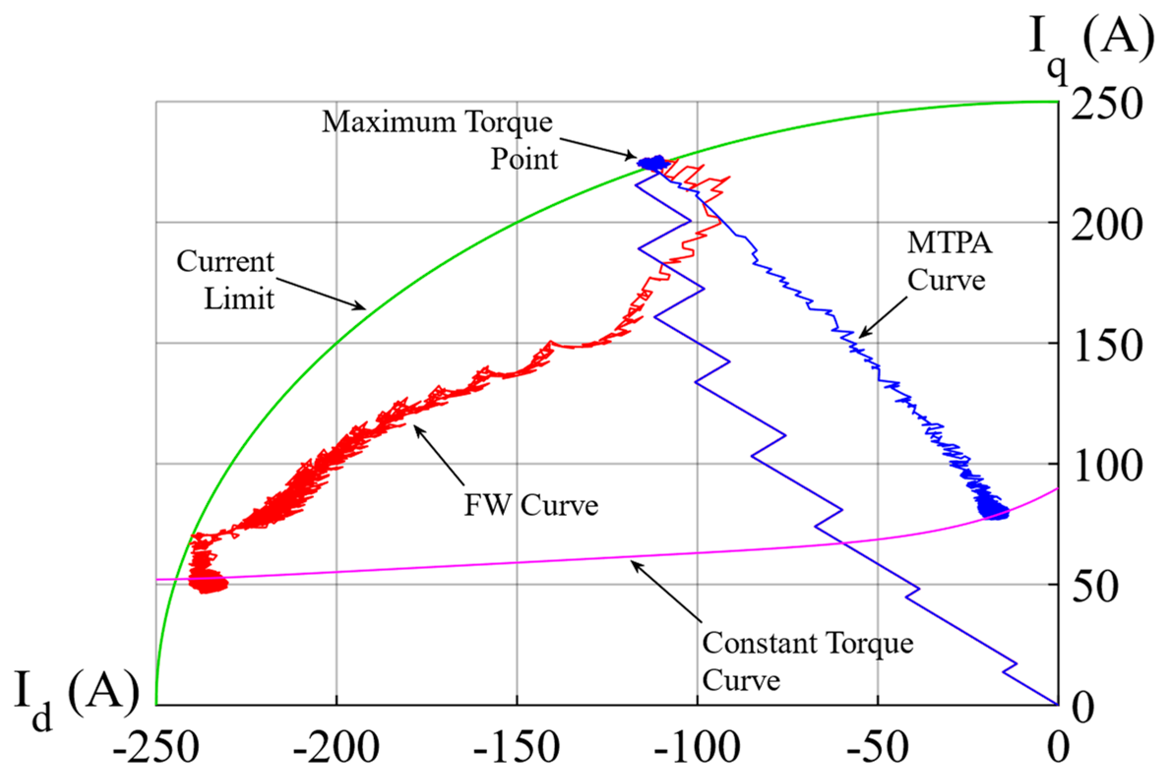
Figure 5 demonstrates the MTPA curve of the dq−axis current trajectories of the step response of the IPMSM in an MTPA control when the motor speed is increased from a standstill to 3500 rpm under a 50 Nm load for this sample case. The motor is operated along the MTPA curve until it reaches the base speed. The dq−axis currents of the motor reach the MTPA point, which intersects with the constant torque curve of the motor at a 50 Nm load in the steady-state point. Thus, the MTPA curve provides the minimum current to achieve the desired torque. Therefore, the motor’s efficiency is increased because the copper losses are minimized. Afterward, the motor speed is increased to 8000 rpm. The operation type of the motor goes from MTPA to FW at the maximum torque point. Similarly, the dq−axis currents of the motor reach the FW point, which intersects with the constant torque curve of the motor at a 50 Nm load at the steady-state point. As a result, a wide speed range can be obtained through the FW control for the IPMSM.

To verify the performance of the proposed adaptive STA-MRAS strategy, it is compared to the TSM-based MRAS, which uses a sliding mode strategy, and the conventional PI-MRAS. The above three strategies are performed at the same parameters of speed and the current controller in an MTPA. The parameters of the adaptive STA-MRAS are designed as $k_1\left(0\right)=3.5$, $k_2=500$, $a=2$, and $l=$ 0.02; the TSM-MRAS parameters are ${\mu }_1=0.2$, ${\mu }_2=1.25$, and $\sigma =0.95$; PI parameters are $k_P=2.2$ and $k_I=0.5$.

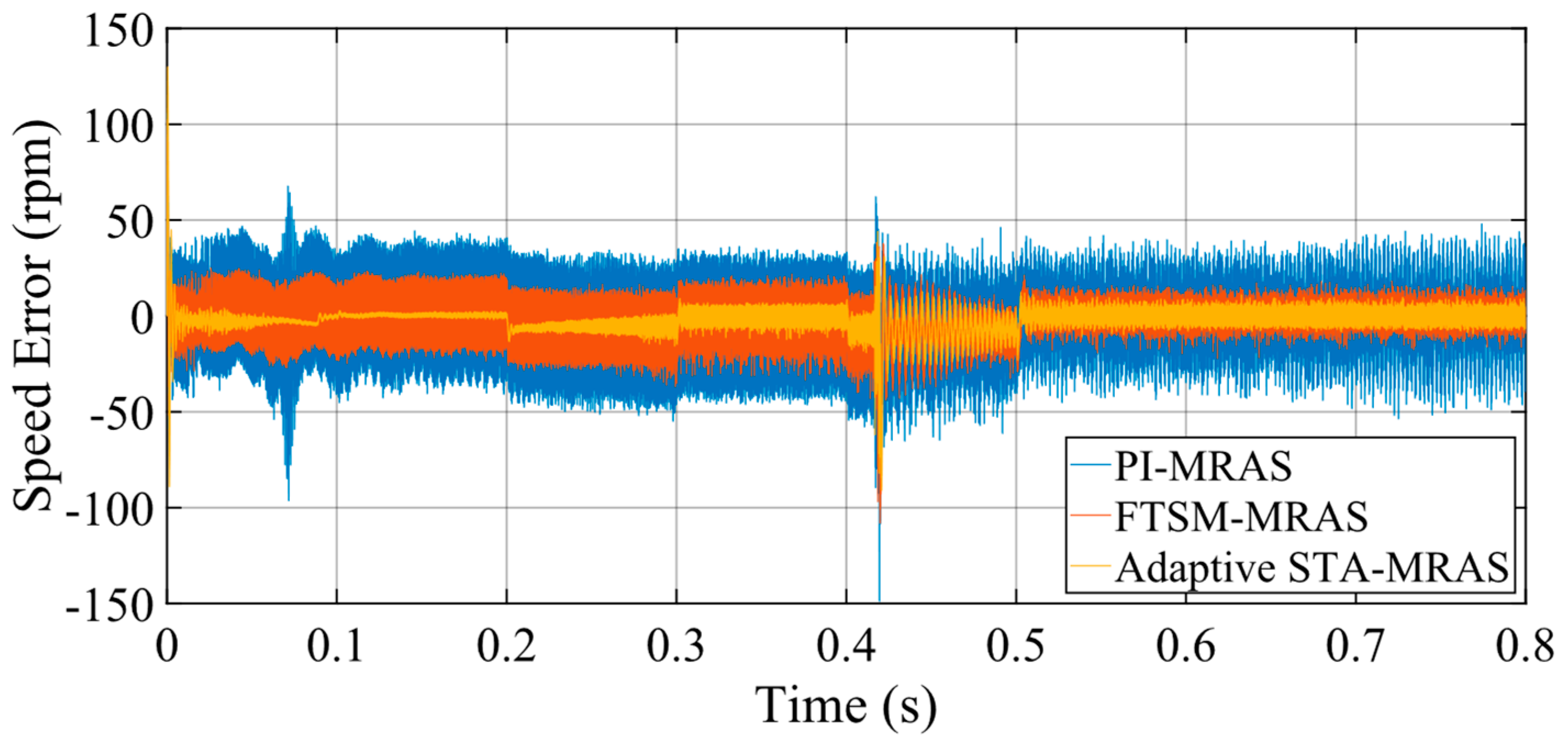
In order to analyze the steady-state and dynamic condition performance of the MRAS methods, the reference speed command is given as follows: it is increased from 0 to 500 rpm for the low-speed condition, then changed from 500 to 3000 rpm for the MTPA control region, and finally raised from 3000 to 6000 rpm for the FW control region. In all cases, the motor was operated at a load torque of 50 Nm. Figure 6 illustrates the response and fluctuations of the rotor speed in the conventional PI-MRAS, FTSM-MRAS, and proposed adaptive STA-MRAS.

The speed errors, which are between the actual and estimated speed for the conventional PI-MRAS, FTSM-MRAS, and proposed adaptive STA-MRAS, are depicted in Figure 7. The range of speed fluctuation is ±2 rpm, ±20 rpm, and ±36 rpm at 500 rpm under the adaptive STA-MRAS, FTSM-MRAS, and PI-MRAS, respectively. The errors of the three methods are around ±6 rpm, ±20 rpm, and ±36 rpm at 3000 rpm, respectively. Finally, the adaptive STA-MRAS considerably reduces the speed error compared with the other MRAS strategies by ±7 rpm at 6000 rpm. The speed error is ±10 rpm in the FTSM-MRAS at 6000 rpm. Additionally, the maximum speed error is ±33 at 6000 rpm when the PI-MRAS is implemented.

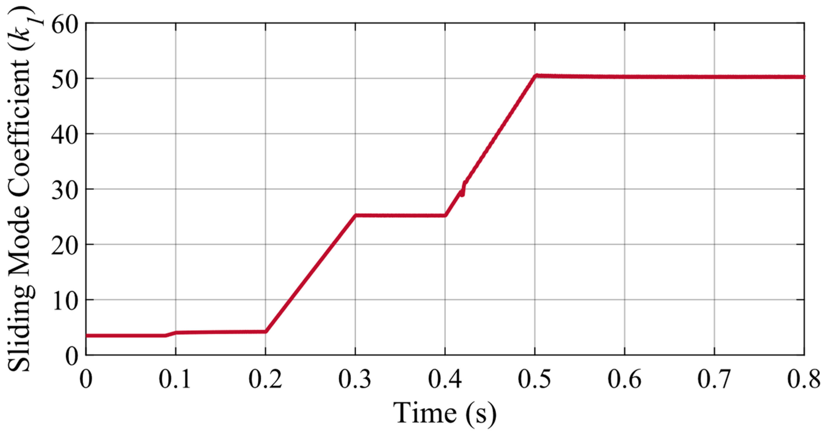
The proposed adaptive STA-MRAS causes less position estimation error than the STA-MRAS with a constant sliding mode coefficient [36]. To suppress the chattering effect in both the low-speed range and the high-speed range, the $k_1$ coefficient is adjusted according to the rotor speed. The sliding mode coefficient $k_1$ has a constant value of approximately 7% of the rated speed. In other words, $k_1$ has a positive initial value $k_1=l{\widehat{\omega }}_r+k_1\left(0\right)$. That is because the coefficient $k_1$ is initialized with a fixed value to prevent the rotor speed from becoming unstable due to the system, which may be unstable at the starting condition. It is obvious that the adaptive STA-MRAS works well, as shown in Figure 6 and Figure 7. Additionally, Figure 8 demonstrates the sliding mode coefficient $k_1$, which varies with the rotor speed of the proposed adaptive STA-MRAS according to the conditions as presented in Figure 6. Additionally, it can be seen that the estimated speed oscillates along at a time of transition from the MTPA to FW control region due to its control algorithm for all observers, between 0.415 s and 0.425 s, as depicted in Figure 6c.

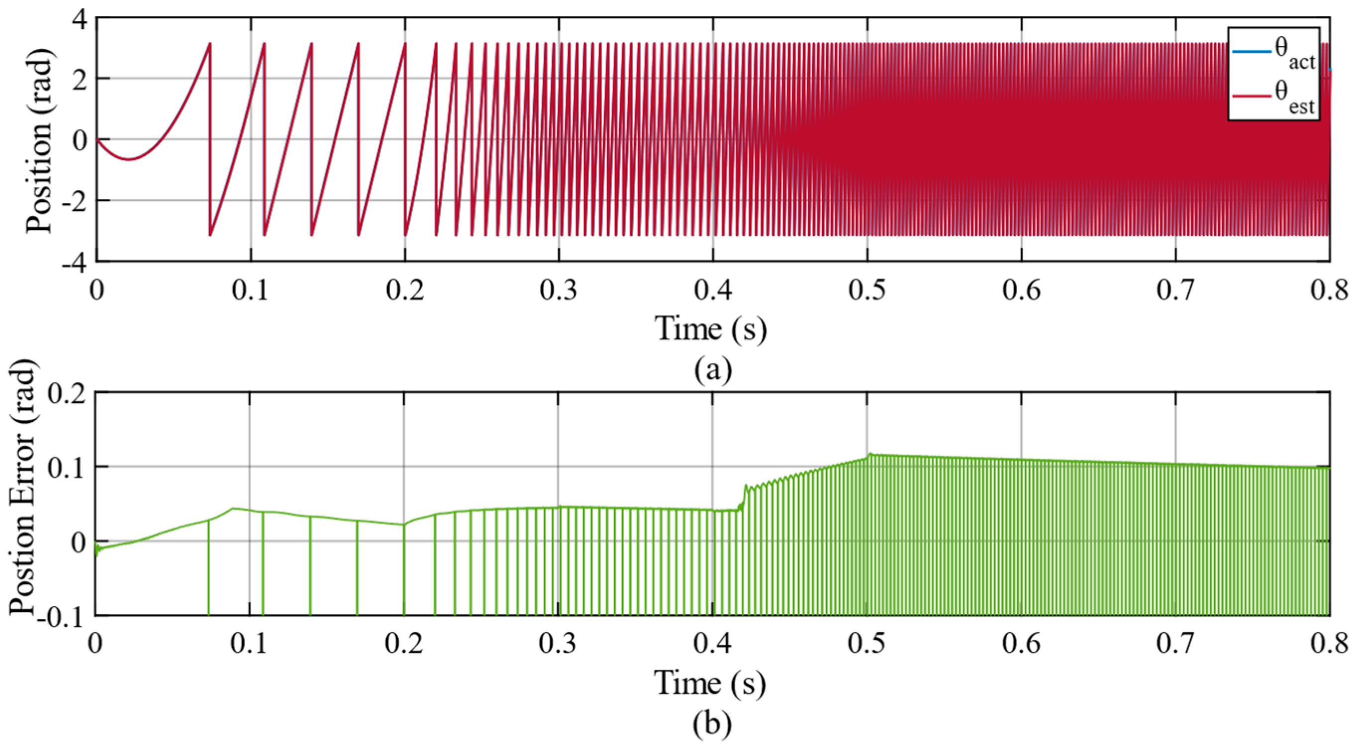
The position estimation error of the proposed adaptive STA-MRAS is depicted in Figure 9. The position error increases as the motor speed increases, especially in the FW region for all observer strategies. The maximum position error oscillates around 0.1 rad at 6000 rpm for the adaptive STA-MRAS from 0.5 s to 0.8 s. Figure 10 displays the position estimation error of the FTSM-MRAS, which is within around 0.15 rad at 6000 rpm from 0.5 s to 0.8 s. Furthermore, the position error is about 0.05 rad at 6000 rpm from 0.5 s to 0.8 s for PI-MRAS, as illustrated in Figure 11. The adaptive STA-MRAS has a smaller chattering effect than the FTSM-MRAS for the rotor position estimation in sliding mode methods. In addition, the PI has a smaller deviation in the estimation of the rotor position than the others. However, the adaptive STA-MRAS, which estimates the rotor position as smoother and more stable when tracking the actual position, increases the performance of the IPMSM, such as by reducing current harmonics, torque ripple, etc.

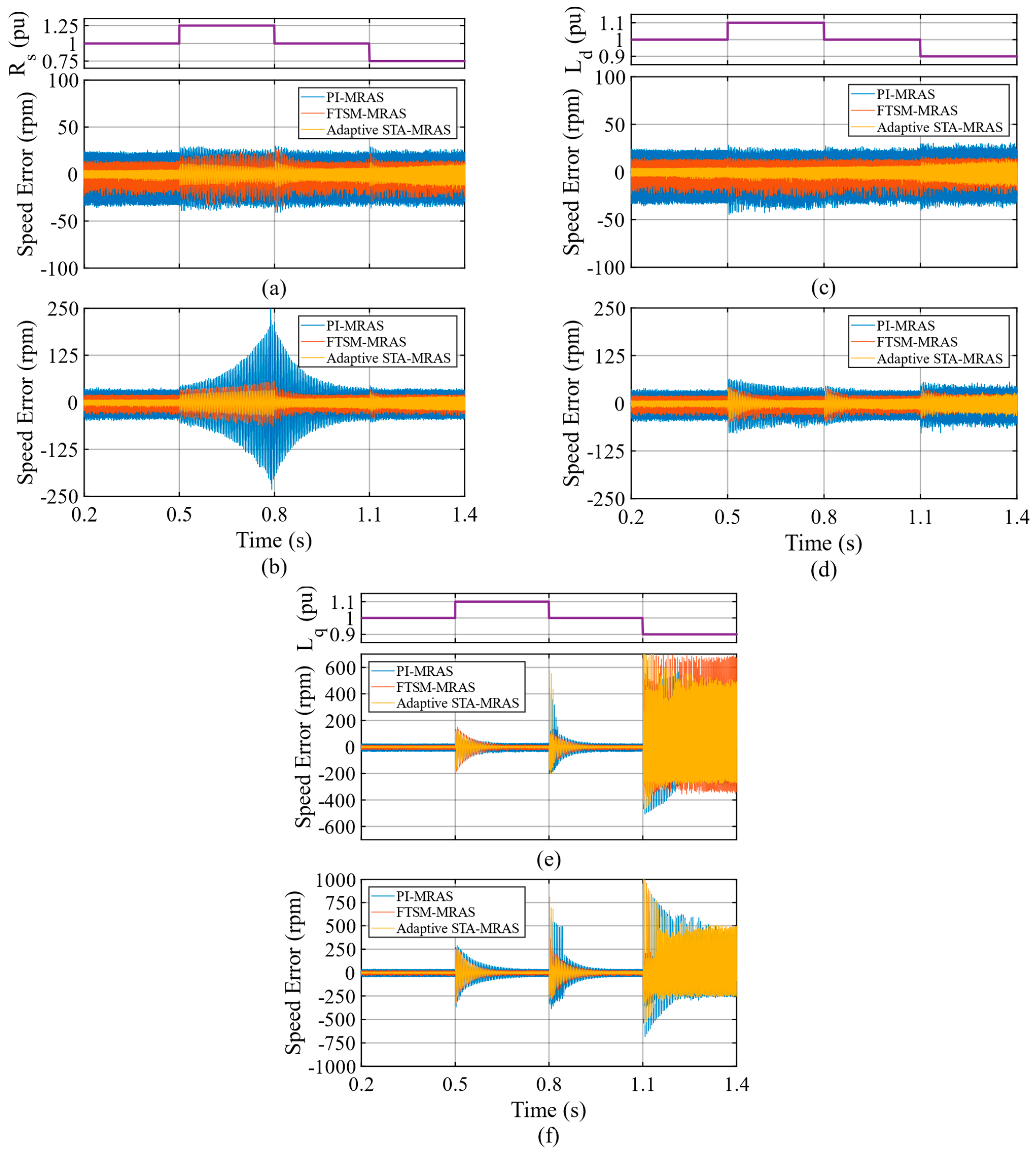
The mismatch between motor and observer parameters causes a rotor position estimation error. Figure 12 depicts the performance of the MRAS observers under model mismatches at 3000 rpm under both 25 Nm and 50 Nm load torque. The stator resistance $R_s$ varies between 0.75 and 1.25 pu. Furthermore, the dq−axis inductances vary within 10% of the original values. The MRAS observers can retain strong robustness during the variation of the $R_s$ without online estimation of the stator resistance. In particular, the adaptive STA-MRAS converges faster to the steady state while the speed error is in a more acceptable range than the other methods during the stator resistance parameter changes. However, the accuracy of the q-axis inductance $L_q$ is required for the MRAS observers in this study. The estimation performance varies with respect to the variation of $L_q$. The MRAS observers can partially maintain their performance when the $L_q$ and $L_d$ parameter values are increased. However, the estimated rotor speed becomes unacceptable when $L_q$ is decreased, unlike $L_d$. When the load torque is increased, as seen in Figure 12b,d,f, the convergence time of the incorrectly estimated rotor speed to the actual rotor speed becomes longer due to the step change in the parameters. Furthermore, the speed fluctuations increase with parameter changes under increasing load torque. Generally, compared to PI-MRAS and FTSM-MRAS, the adaptive STA-MRAS performs with better robustness towards inductance and resistance variation. Therefore, online parameter estimation is necessary to enhance speed accuracy and system stability.

The simulation results demonstrate that the proposed STA-MRAS strategy exhibits reducing speed ripples for an IPMSM controlled in a wide-speed range. The following simulation analyzes the performance of the adaptive STA-MRAS when the motor speed is adjusted by considering the electric vehicle velocity and its transmission system in the drive cycles, which have dynamic load and speed conditions. Therefore, the ECE-15 and EUDC drive cycles (Extra Urban Driving Cycle) have been employed for examining the performance of the proposed adaptive STA-MRAS in electric vehicle (EV) applications. A simplification is made by neglecting the headwind blows and accepting the slope angle as 0°.

Table 2. Parameters of the electric vehicle.

Symbol	Parameter	Value
$m_v$	Vehicle total mass	1313 kg
$A_f$	Vehicle frontal area	1.746 m2
$g_{dr}$	Gear ratio	5
$\rho$	Air mass density	1.225 kg/m3
${\eta }_{dr}$	Transmission efficiency	0.95
$r_w$	Radius of the wheels	0.29 m
$C_d$	Aerodynamic drag coefficient	0.3
$f_r$	Rolling resistance coefficient	0.009
$g$	Gravitational acceleration	9.8 m/s2

illustrates the vehicle parameters utilized in the simulation [34].

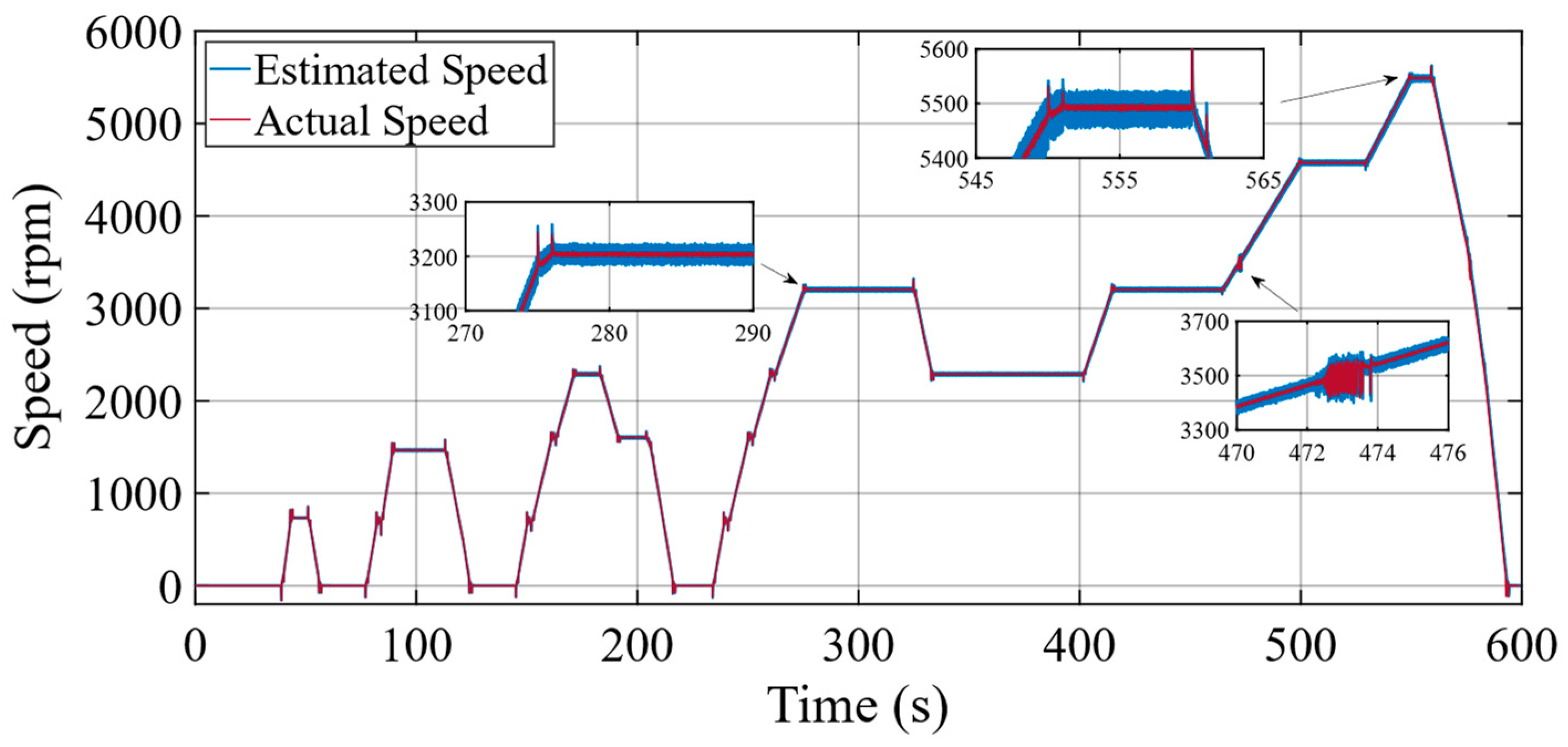
In this paper, the IPMSM operates under MTPA control up to the nominal speed of the motor, which corresponds to 77 km/h of vehicle velocity. Above the nominal speed, FW control is employed. Furthermore, the maximum speed of the EUDC is 120 km/h, which is equal to almost 5500 rpm for the IPMSM.

Figure 13, Figure 14 and Figure 15 demonstrate the rotor speed, developed electromagnetic torque, and dq−axis current obtained by the adaptive STA-MRAS, respectively. Furthermore, the rotor speed fluctuated during the transition from the MTPA to the FW control region operation and vice versa because the reference speed oscillated around the base speed, from time 472 s to 474 s, as illustrated in Figure 13. Moreover, the dq−axis current, which oscillates, causes torque ripples in transient states, as shown in Figure 14 and Figure 15. The absolute value of the d-axis component increases quickly when entering the FW region. For this reason, the torque fluctuation will be bigger for the IPMSM above the base speed. Also, the estimation errors of the adaptive STA-MRAS for different conditions in the drive cycle are summarized in

Table 3. Performance of the adaptive STA-MRAS for MTPA and FW control in steady-state conditions.

Operating Condition	Torque				Speed Error	${\mathbf{I}}_{\mathbf{d}\_\mathbf{A}\mathbf{v}\mathbf{g}}$	${\mathbf{I}}_{\mathbf{d}\_\mathbf{R}\mathbf{i}\mathbf{p}\mathbf{p}\mathbf{l}\mathbf{e}}$	${\mathbf{I}}_{\mathbf{q}\_\mathbf{A}\mathbf{v}\mathbf{g}}$	${\mathbf{I}}_{\mathbf{q}\_\mathbf{R}\mathbf{i}\mathbf{p}\mathbf{p}\mathbf{l}\mathbf{e}}$
	Max. Value	Min. Value	Mean Value	MAPE
3200 rpm, 14.5 Nm (in MTPA)	18.65 Nm	11.84 Nm	15.27 Nm	6.88%	35 rpm	−1.29 A	1.92 A	25.61 A	1.56 A
5500 rpm, 28.9 Nm (in FW)	36.38 Nm	25.02 Nm	30.46 Nm	6.74%	60 rpm	−211.42 A	2.47 A	31.51 A	1.93 A

. Table 3 reports torque performances such as max, min, mean values, and mean absolute percentage error (MAPE) alongside speed and current performance for the modified STA-based MRAS. The MTPA control region is more stable than the FW region for the IPMSM in terms of ripple of speed, torque, and current. Nevertheless, the modified STA-MRAS gives almost the same performance in terms of the mean absolute percentage error of the torque for both operating conditions.

7. Conclusions

This article presents the MRAS strategy, which is based on the adaptive STA approach for sensorless control of the IPMSM operating under the MTPA control algorithm. The proposed adaptive STA-MRAS is compared with both the conventional PI-MRAS and the FTSM-MRAS. Hereby, the FTSM-MRAS is utilized to compare with the adaptive STA-MRAS as a method using the sliding mode strategy. The results demonstrate the adaptive STA-MRAS can be provided with speed estimation accuracy and robustness of the system under parameter variation to other strategies without the online estimation of motor parameters. Additionally, the simulation results conclude that the proposed STA-MRAS has reduced the chattering effect, and the estimated rotor speed is more accurate in both dynamic and steady-state conditions.

Moreover, the performance of the modified STA-MRAS has been examined in the traction drive of the electric vehicle under the combined ECE and EUDC drive cycles. The simulation tests have confirmed that the proposed strategy exhibits acceptable estimation errors and has accurate estimation capability under different speed and load conditions.

References

1. Liu, J.; Gong, C.; Han, Z.; Yu, H. IPMSM Model Predictive Control in Flux-Weakening Operation Using an Improved Algorithm. IEEE Trans. Ind. Electron. 2018, 65, 9378–9387. [Google Scholar] [CrossRef]
2. Guo, L.; Parsa, L. Model Reference Adaptive Control of Five-Phase IPM Motors Based on Neural Network. IEEE Trans. Ind. Electron. 2012, 59, 1500–1508. [Google Scholar] [CrossRef]
3. Bıçak, A.; Gelen, A. Sensorless Direct Torque Control Based on Seven-Level Torque Hysteresis Controller for Five-Phase IPMSM Using a Sliding-Mode Observer. Eng. Sci. Technol. Int. J. 2021, 24, 1134–1143. [Google Scholar] [CrossRef]
4. Lin, F.J.; Liao, Y.H.; Lin, J.R.; Lin, W.T. Interior Permanent Magnet Synchronous Motor Drive System with Machine Learning-Based Maximum Torque per Ampere and Flux-Weakening Control. Energies 2021, 14, 346. [Google Scholar] [CrossRef]
5. Foo, G.; Rahman, M.F. Sensorless Vector Control of Interior Permanent Magnet Synchronous Motor Drives at Very Low Speed without Signal Injection. IET Electr. Power Appl. 2010, 4, 131–139. [Google Scholar] [CrossRef]
6. Justo, J.J.; Mwasilu, F.; Kim, E.K.; Kim, J.; Choi, H.H.; Jung, J.W. Fuzzy Model Predictive Direct Torque Control of IPMSMs for Electric Vehicle Applications. IEEE/ASME Trans. Mechatron. 2017, 22, 1542–1553. [Google Scholar] [CrossRef]
7. Liang, D.; Li, J.; Qu, R. Sensorless Control of Permanent Magnet Synchronous Machine Based on Second-Order Sliding-Mode Observer With Online Resistance Estimation. IEEE Trans. Ind. Appl. 2017, 53, 3672–3682. [Google Scholar] [CrossRef]
8. Wu, S.; Zhang, J.; Chai, B. Adaptive Super-Twisting Sliding Mode Observer Based Robust Backstepping Sensorless Speed Control for IPMSM. ISA Trans. 2019, 92, 155–165. [Google Scholar] [CrossRef] [PubMed]
9. Abo-Khalil, A.G.; Eltamaly, A.M.; Alsaud, M.S.; Sayed, K.; Alghamdi, A.S. Sensorless Control for PMSM Using Model Reference Adaptive System. Int. Trans. Electr. Energy Syst. 2021, 31, e12733. [Google Scholar] [CrossRef]
10. Chen, J.; Chen, S.; Wu, X.; Tan, G.; Hao, J. A Super-Twisting Sliding-Mode Stator Flux Observer for Sensorless Direct Torque and Flux Control of IPMSM. Energies 2019, 12, 2564. [Google Scholar] [CrossRef]
11. Li, L.; Zhou, W.; Bi, X.; Shi, X. Speed Estimation of PMSM Based on a Super-Twisting Slide Mode Observer. Machines 2022, 10, 681. [Google Scholar] [CrossRef]
12. Cao, R.; Jiang, N.; Lu, M. Sensorless Control of Linear Flux-Switching Permanent Magnet Motor Based on Extended Kalman Filter. IEEE Trans. Ind. Electron. 2020, 67, 5971–5979. [Google Scholar] [CrossRef]
13. Khlaief, A.; Boussak, M.; Châari, A. A MRAS-Based Stator Resistance and Speed Estimation for Sensorless Vector Controlled IPMSM Drive. Electr. Power Syst. Res. 2014, 108, 1–15. [Google Scholar] [CrossRef]
14. Badini, S.S.; Verma, V. Parameter Independent Speed Estimation Technique for PMSM Drive in Electric Vehicle. Int. Trans. Electr. Energy Syst. 2021, 31, e13071. [Google Scholar] [CrossRef]
15. Verma, V.; Chakraborty, C. New Series of MRAS for Speed Estimation of Vector Controlled Induction Motor Drive. In Proceedings of the IECON Proceedings (Industrial Electronics Conference), Dallas, TX, USA, 29 October–1 November 2014; Institute of Electrical and Electronics Engineers Inc.: Piscataway, NJ, USA, 2014; pp. 755–761. [Google Scholar]
16. Ravi Teja, A.V.; Verma, V.; Chakraborty, C. A New Formulation of Reactive-Power-Based Model Reference Adaptive System for Sensorless Induction Motor Drive. IEEE Trans. Ind. Electron. 2015, 62, 6797–6808. [Google Scholar] [CrossRef]
17. He, Y.; Wang, J.; Wang, Z.; Wang, H.; Wang, Q.; Wei, D.; Zeng, Z. Speed Observation of High-Speed Permanent Magnet Synchronous Motor Based on Fuzzy MRAS. In Proceedings of the 39th Chinese Control Conference, Shenyang, China, 27–29 July 2020; pp. 3550–3555. [Google Scholar]
18. Jain, M.; Singh, M.; Chandra, A.; Williamson, S.S. Sensorless Control of Permanent Magnet Synchronous Motor Using ANFIS Based MRAS. In Proceedings of the 2011 IEEE International Electric Machines and Drives Conference, IEMDC, Niagara Falls, ON, Canada, 15–18 May 2011; pp. 599–606. [Google Scholar]
19. Azza, H.B.; Zaidi, N.; Jemli, M.; Boussak, M. Development and Experimental Evaluation of a Sensorless Speed Control of SPIM Using Adaptive Sliding Mode-MRAS Strategy. IEEE J. Emerg. Sel. Top. Power Electron. 2014, 2, 319–328. [Google Scholar] [CrossRef]
20. Comanescu, M.; Xu, L. Sliding-Mode MRAS Speed Estimators for Sensorless Vector Control of Induction Machine. IEEE Trans. Ind. Electron. 2006, 53, 146–153. [Google Scholar] [CrossRef]
21. Gabbi, T.S.; Gründling, H.A.; Vieira, R.P. Sliding Mode MRAS Speed Observer Applied to Permanent Magnet Synchronous Motor with Decoupled Current Control. In Proceedings of the IECON Proceedings (Industrial Electronics Conference), Florence, Italy, 23–26 October 2016; IEEE Computer Society: Piscataway, NJ, USA, 2016; pp. 2929–2934. [Google Scholar]
22. Kouriche, L.; Messlem, Y. MRAS-Super Twisting Sliding Mode Observer for Speed Sensorless Vector Control of Induction Motor Drive. Prz. Elektrotech. 2021, 97, 121–127. [Google Scholar] [CrossRef]
23. Feng, W.; Bai, J.; Zhang, J. Full-Order Adaptive Observer for Interior Permanent-Magnet Synchronous Motor Based on Novel Fast Super-Twisting Algorithm. Meas. Control 2023, 56, 93–113. [Google Scholar] [CrossRef]
24. Soufyane, B.; Abdelhamid, R.; Smail, Z. Adaptation Mechanism Techniques for Improving a Model Reference Adaptive Speed Observer in Wind Energy Conversion Systems. Electr. Eng. 2020, 102, 1621–1637. [Google Scholar] [CrossRef]
25. Yu, S.; Yu, X.; Shirinzadeh, B.; Man, Z. Continuous Finite-Time Control for Robotic Manipulators with Terminal Sliding Mode. Automatica 2005, 41, 1957–1964. [Google Scholar] [CrossRef]
26. Huang, H.; Tu, Q.; Pan, M.; Jiang, C.; Xue, J. Fast Terminal Sliding Mode Control of Permanent Magnet In-Wheel Motor Based on a Fuzzy Controller. Energies 2020, 13, 188. [Google Scholar] [CrossRef]
27. Wang, B.; Luo, C.; Yu, Y.; Wang, G.; Xu, D. Antidisturbance Speed Control for Induction Machine Drives Using High-Order Fast Terminal Sliding-Mode Load Torque Observer. IEEE Trans. Power Electron. 2018, 33, 7927–7937. [Google Scholar] [CrossRef]
28. Li, L.; Liu, Q. Research on IPMSM Drive System Control Technology for Electric Vehicle Energy Consumption. IEEE Access 2019, 7, 186201–186210. [Google Scholar] [CrossRef]
29. Morimoto, S.; Sanada, M.; Takeda, Y. Wide-Speed Operation of Interior Permanent Magnet Synchronous Motors with High-Performance Current Regulator. IEEE Trans. Ind. Appl. 1994, 30, 920–926. [Google Scholar] [CrossRef]
30. Wagg, D.J. Adaptive Control of Nonlinear Dynamical Systems Using a Model Reference Approach. Meccanica 2003, 38, 227–238. [Google Scholar] [CrossRef]
31. Wang, B.; Shao, Y.; Yu, Y.; Dong, Q.; Yun, Z.; Xu, D. High-Order Terminal Sliding-Mode Observer for Chattering Suppression and Finite-Time Convergence in Sensorless SPMSM Drives. IEEE Trans. Power Electron. 2021, 36, 11910–11920. [Google Scholar] [CrossRef]
32. Levant, A. Sliding Order and Sliding Accuracy in Sliding Mode Control. Int. J. Control 1993, 58, 1247–1263. [Google Scholar] [CrossRef]
33. Moreno, J.A.; Osorio, M. A Lyapunov Approach to Second-Order Sliding Mode Controllers and Observers. In Proceedings of the 2008 47th IEEE Conference on Decision and Control, Cancun, Mexico, 9–11 December 2008; pp. 2856–2861. [Google Scholar]
34. Nam, K.H. AC Motor Control and Electric Vehicle Applications; CRC Press: Boca Raton, FL, USA, 2018. [Google Scholar]
35. Jung, S.Y.; Hong, J.; Nam, K. Current Minimizing Torque Control of the IPMSM Using Ferrari’s Method. IEEE Trans. Power Electron. 2013, 28, 5603–5617. [Google Scholar] [CrossRef]
36. Liang, D.; Li, J.; Qu, R.; Kong, W. Adaptive Second-Order Sliding-Mode Observer for PMSM Sensorless Control Considering VSI Nonlinearity. IEEE Trans. Power Electron. 2018, 33, 8994–9004. [Google Scholar] [CrossRef]
Figure 1. Equivalent circuit model of IPMSM (a) d-axis circuit (b) q-axis circuit.
Machines 11 00871 g001
Figure 2. The MRAS speed observer.
Machines 11 00871 g002
Figure 3. Acting forces on a vehicle moving uphill.
Machines 11 00871 g003
Figure 4. The scheme of the sensorless MTPA control with the MRAS strategy.
Machines 11 00871 g004
Figure 5. The dq−axis current components loci based on step response.
Machines 11 00871 g005
Figure 6. The speed response of MRAS observers at various speed conditions under fixed load and (ad) zoomed view of speed responses.
Machines 11 00871 g006aMachines 11 00871 g006b
Figure 7. Error between the estimated speed and actual speed.
Machines 11 00871 g007
Figure 8. The varying of the sliding mode coefficient of the adaptive STA.
Machines 11 00871 g008
Figure 9. The simulation results of the proposed adaptive STA−MRAS strategy. (a) The actual and the estimated rotor electrical position, and (b) the error waveform of the rotor position.
Machines 11 00871 g009
Figure 10. The simulation results of FTSM−MRAS strategy. (a) The actual and the estimated rotor electrical position, and (b) the error waveform of the rotor position.
Machines 11 00871 g010
Figure 11. The simulation results of PI−MRAS strategy. (a) The actual and the estimated rotor electrical position, and (b) the error waveform of the rotor position.
Machines 11 00871 g011
Figure 12. Results of the MRAS observers under model mismatches at 3000 r/min (a) ±25% variation of the stator resistance at 25 Nm, (b) ±25% variation of the stator resistance at 50 Nm, (c) ±10% variation of the d−axis inductance at 25 Nm, (d) ±10% variation of the d−axis inductance at 50 Nm, (e) ±10% variation of the q−axis inductance at 25 Nm, and (f) ±10% variation of the q−axis inductance at 50 Nm.
Machines 11 00871 g012
Figure 13. Mechanical rotor speed under ECE and EUDC drive cycles.
Machines 11 00871 g013
Figure 14. Electromagnetic torque under ECE and EUDC drive cycles.
Machines 11 00871 g014
Figure 15. The dq−axis current components under ECE and EUDC drive cycles.
Machines 11 00871 g015