Article

Robust Nonlinear Trajectory Controllers for a Single-Rotor UAV with Particle Swarm Optimization Tuning

by
Patricia Portillo
1,
Luis E. Garza-Castañón
1,*,
Luis I. Minchala-Avila
2,
Adriana Vargas-Martínez
1,
Vicenç Puig Cayuela
3 and
Pierre Payeur
4
1
School of Engineering and Sciences, Tecnologico de Monterrey, Eugenio Garza Sada 2501, Monterrey 64849, Mexico
2
Department of Electrical Engineering, Electronics and Telecommunications, Universidad de Cuenca, Cuenca 010101, Azuay, Ecuador
3
Supervision, Safety and Automatic Control Research Center (CS2AC), Universitat Politécnica de Catalunya (UPC), Rambla Sant Nebridi, 22, 08222 Terrassa, Barcelona, Spain
4
School of Electrical Engineering and Computer Science, University of Ottawa, 800 King Edward, Ottawa, ON K1N 6N5, Canada
*
Author to whom correspondence should be addressed.
Machines 2023, 11(9), 870; https://doi.org/10.3390/machines11090870
Submission received: 4 July 2023 / Revised: 23 August 2023 / Accepted: 25 August 2023 / Published: 29 August 2023
(This article belongs to the Special Issue Robust Control of Robotic and Complex Mechatronic Systems)

Abstract

:
This paper presents the utilization of robust nonlinear control schemes for a single-rotor unmanned aerial vehicle (SR-UAV) mathematical model. The nonlinear dynamics of the vehicle are modeled according to the translational and rotational motions. The general structure is based on a translation controller connected in cascade with a P-PI attitude controller. Three different control approaches (classical PID, Super Twisting, and Adaptive Sliding Mode) are compared for the translation control. The parameters of such controllers are hard to tune by using a trial-and-error procedure, so we use an automated tuning procedure based on the Particle Swarm Optimization (PSO) method. The controllers were simulated in scenarios with wind gust disturbances, and a performance comparison was made between the different controllers with and without optimized gains. The results show a significant improvement in the performance of the PSO-tuned controllers.

1. Introduction

During the last decade, we have seen the presence of unmanned aerial vehicles (UAVs) in different applications, whether in the commercial industry or high-end application fields such as the military, avionics, and artificial intelligence [1]. A UAV is a pilotless aircraft with the ability to fly and stay in a hover state without any human interaction. They are piloted remotely through control commands from a ground station [2].
In general, depending on the characteristics of the UAV, its application, speed, weight, and operation vary. UAVs are generally divided into four categories: fixed wing, fixed-wing hybrid, multirotor, and single rotor. Fixed-wing UAVs are vehicles based on wings, a main body, a motor, and a propeller. This type of UAV requires unique and extensive training to pilot them. One of its main advantages is the flight time of several hours. However, this vehicle is not able to perform a backward flight, hover, or rotate. The next type is the fixed-wing hybrid, which combines automated and manual gliding. Although that is an advantage, this type of UAV could be better at forward flight and hovering. Multirotor vehicles are the most common in the industry. There are different types of multirotors, and they are generally classified by the number of rotors or propellers they have. There are tricopters, quadcopters, hexacopters, and octocopters. The most used are quadcopters since they have a vertical landing, small size, and simple structure [2,3]. The last one is the single-rotor UAV, which has a single rotor as its name mentions. This type of UAV is less developed than the others since it is complex to design. Nevertheless, they have distinct advantages, like a heavy payload, a mixture of hovering with long endurance, and fast forward flight [4].
In recent years, it has been concluded that UAVs are no longer sufficient to fly autonomously, and more advanced technologies are needed to bring innovations and improvements to achieve more complex goals. While UAVs excel in speed and flight duration, innovative solutions are imperative to address their limited robustness, a pivotal consideration for large-scale deployment and diverse task completion [2].
It is common to assume that a single-rotor system resembles a conventional helicopter; however, this assumption only holds partially. The fundamental distinction lies in their dynamic configuration and weight-handling approaches [5]. Unlike helicopters, which employ a primary rotor and tail rotor to counteract asymmetry and reaction torque, single-rotor systems rely on fins or control surfaces to achieve stability and direction [4].
Helicopter dynamics revolve around the lift and control generated by the main rotor, counteracted by tail-rotor reaction torque [6]. Conversely, single-rotor systems employ fins and control surfaces to manipulate airflow, enabling precise aircraft control. Furthermore, single-rotor systems, generally lighter than traditional helicopters, leverage more efficient configurations and sophisticated control systems, compensating for dynamic and weight differences [4].

1.1. Single-Rotor UAV

Single-rotor UAVs only have one propeller, and although it could be seen as a disadvantage since it would lose maneuverability, in reality, the energy use also decreases. Using only one rotor increases the flight efficiency, reduces energy consumption, and allows for an important feature: the VTOL (vertical take-off and landing) [7]. Different single-rotor UAV designs have been introduced over the years. A single rotor composed of two fixed-wing airplanes was analyzed in [8], in which two attached rotating airplanes can be modeled and controlled. Another variation studied is the single-rotor aerial vehicle, which features a model with a single rotor and a tail rotor [9]. In [4], a different approach based on the design of a single-rotor VTOL is presented. This design is based on thrust vectoring through a single propeller and four deflecting fins actuated by small motors. In that work, the process design is simplified to obtain lower costs and an increase in the number of applications.
Path following and trajectory tracking constitute primary control challenges for UAVs [10]. The PID (Proportional Integral Derivative) controller is commonly used in UAVs [11] due to its versatility and applicability to various UAV variants. However, the PID has limitations in handling complex systems, uncertainties, disturbances, and nonlinearities, making more robust control techniques desirable. The PID does not require a mathematical model of the system but has limitations when systems are complex. Changes in the system parameters can affect the stability and performance of the control if the parameters are not tuned properly. In addition, the PID is not efficient for handling uncertainties and disturbances compared to other more robust controllers. Because the PID is designed on linear assumptions, it has difficulties controlling nonlinear systems. The elimination of steady-state errors is also a limitation that reduces the control performance [12]. For this reason, more robust nonlinear control techniques are considered in this work to deal with such issues.
This work explores robust nonlinear control techniques such as the Adaptive Sliding Mode (ASM) and Super Twisting (ST) for single-rotor UAVs. ST is a control technique used for nonlinear dynamic systems based on the theory of sliding mode and trajectory tracking to zero. Several approaches have been used in the literature to quantify the position control of small-rotor UAVs. In [13], it is demonstrated that ST control is one of the most powerful second-order sliding mode controllers for systems with a relative degree equal to one. The main contribution of this work is the robust ST control for solving the attitude-tracking problem of a quadrotor subject to perturbations. Limitations in the controller are also observed. The main one is the presence of chattering [14]. Although the controller is shown to be robust, it has limitations with regard to working with uncertainties, requiring extensive knowledge for tuning [15].
Sliding mode techniques have also been applied in the control of UAVs. For instance, [16] presents a bond graph (BG) model and a robust cascaded controller for a twin-rotor system. The BG model accounts for all the energetic and dynamical couplings. An adaptive integral backstepping sliding mode controller is used in an outer loop to control the yaw and pitch dynamics. Although the proposed controller was able to obtain less chatter and lower the following error than the others during experiments, it did so at the expense of an increased response time, which implies a trade-off between accuracy and speed. In [17], a robust and fault-tolerant controller is designed to determine the position and attitude dynamics by using a higher-order integral dynamic sliding mode controller. The proposed method requires redundant actuators, which increases the cost of implementation. Here, the performance of finite-time disturbance observers used to estimate the combined effects of parametric uncertainty, external disturbances, and actuator faults is satisfactory, but the estimators start deteriorating after intermittent faults. Additionally, in [18], the attitude-position tracking control of fully actuated multirotor aerial vehicles equipped with fixed rotors and subject to matched model uncertainties and disturbances is presented. Here, a joint geometric attitude-position control law is designed by using a multi-input smooth second-order sliding mode strategy. The simulations show that the proposed method reduces the chattering and improves the tracking performance in comparison with Super Twisting and second-order sliding mode controllers, but it still presents oscillatory behavior, which is mainly caused by the unmodeled rotor dynamics. Finally, ref. [19] presents the development of a terminal sliding mode attitude-position quaternion-based control of a quadrotor unmanned aerial vehicle (UAV). The dynamics of the UAV are split into an attitude and position loop to design independent control laws. The control law implemented for each loop is the hybrid terminal sliding mode and quaternion controller. The results obtained in simulations showed better performance when compared with a higher-order sliding mode controller, but like the other previously mentioned works, they did not test the method with sustained wind gust disturbances as we did in our work.
Another nonlinear control technique for complex dynamic systems is the Adaptive Sliding Mode [20]. It also has the ability to handle uncertainties in the system model. It is based on the theory of bringing the system’s state to a sliding surface controlled by a linear controller [21]. The ASM has the ability to provide smooth and precise control, but the outstanding feature of the ASM is its ability to reduce the chattering effect. This effect is an unwanted vibration in the ST controller under certain conditions. The ASM has an inherent disturbance rejection capability to compensate for disturbances without requiring additional control action [22].
Regarding the implementation of the ASM in the SR-UAV, it is beneficial due to the nonlinear complexity of the system and the variable perturbations it faces in different flight conditions. The adaptive capability of the ASM is presented as a prosperous solution for controlling a nonlinear system such as the SR-UAV [23]. However, the limitation of the complexity of the ASM implementation must be kept in mind, as well as the requirement for the selection of the controller parameters and the detailed knowledge of the system model [24].
To deal with uncertainty and external disturbances in UAVs, there have been previous works; for instance, ref. [25] addresses the design of a robust controller based on nonlinear estimators for a quadrotor. This controller ensures the tracking of desired references even with parameter variations and external disturbances. It uses high-order sliding mode estimators to estimate the disturbances, which can then be canceled by the controller, thus improving the dynamic behavior of the controlled system. However, experiments to show the performance of the proposed controller in more complex trajectories, as the helical route we use in our testing, are missing. Another type of perturbation implementation is based on the Von Karman wind model [26]. This model allows one to understand and characterize different types of wind, such as steady wind, turbulent flow, wind speed variations, and a propulsor vortex. By combining this model with the mathematical representation of the UAV, the motion of the UAV in a wind field can be illustrated from three different perspectives: speed, force, and energy.

1.2. Particle Swarm Optimization

One of the main problems found in UAV controllers is the tuning process over which the controller gains are adjusted by trial-and-error to minimize the settling time and the corresponding oscillations of the closed-loop system. Many gains need to be adjusted depending on the number and the type of controllers in the system. Each set of gains represents a new possible scenario to obtain the best conditions for the experiment, which can make tuning rather long, tedious, and costly. Particle Swarm Optimization is a global metaheuristic optimization method that belongs to the family of algorithms based on the swarm intelligence concept introduced by Kennedy and Eberhart [27]. This method is based on the concept of swarming, which is inspired by the collective behavior of social animals, especially bird flocks and fish schools. A swarm is a population of agents which perform tasks by interacting locally with each other and with an environment. There is no central control, and their behavior arises from stochastic local self-organization and interaction. These swarm individuals could be more satisfied with limited capabilities; the goal is achieved by exchanging information obtained through the behavioral and interaction parameters [28]. Specifically, this type of optimization is suitable for solving problems where the optimal solution is a point in a multidimensional parameter space. Each particle is evaluated to determine its fitness value. At each iteration, a fitness value is calculated and compared with the previous value to obtain the best one. This social interaction is direct, which means that each particle is influenced by its memory (the best solution so far) and by those of the other agents. Individual and global best positions are updated, where if a stop criterion is not met, the velocity and position are updated to create a new swarm. The two fundamental operations are the velocity and position update. The actual velocity depends on the old velocity, the individual particle’s experience, and the whole swarm’s experience. Each term has an associated weight constant [29].
PSO has been used in the control of UAVs due to the difficulty of adjusting the parameters of the controllers. For instance, the camera-position control on a UAV is presented in [30]. The designed PID controller keeps the camera stable. Traditional fitting methods and evolutionary/bioinspired algorithms such as PSO are discussed in this article. It is highlighted that PSO is used due to its stable convergence, both in terms of its dynamic and static performance and its good computational efficiency, which allows for improving the system performance through error minimization. The research concluded that the PSO-tuned PID controller offers accuracy and convergence stability, which makes it the preferred option. In [30], PSO is applied to camera-position control, offering stable convergence and improved system performance compared to manual tuning. The approach proposed in [31] is the modified PSO (MOPSO), which optimizes the gains of a PID controller for an AR drone quadcopter. The MOPSO algorithm demonstrates the efficient adjustment of the PID parameters, resulting in no overshoot, zero steady-state errors, and a short rise time. Similarly, in [32], PSO is used to optimize parameters in a four-rotor PID controller, achieving a shorter tuning time and reduced overshoot. However, despite these achievements, there is limited research on using PSO in UAV control with nonlinear methods. For instance, in [33], PSO is employed to tune the gains of three nonlinear control strategies for quadrotor attitude control and trajectory tracking. The GTNC controller stands out as it consistently converges to the desired attitude and effectively reduces the position error and basin of attraction to zero, making it more reliable at high speeds. However, it requires more processing time compared to other controllers. In [34], a control strategy is proposed for a quadrotor with a sliding mode controller (SMC) that will use the gains obtained from Lyapunov stability analysis and PSO. The controller is shown to be stable with the gains obtained from PSO. A PID controller is also added to the SMC control law when a fault is detected to stabilize it. The results show that this control technique meets the desired requirements given the gains obtained by the PSO algorithm.
The main contributions of this paper strengthen our existing knowledge in two aspects:
  • First, in this research, robust nonlinear controllers are used. To the best of our knowledge, none of these approaches have been applied before with single-rotor UAVs. We show that these controllers are effective in improving SR-UAV performance, especially under wind gusts disturbances.
  • Second, we prove that the gain values obtained with the PSO algorithm satisfy Lyapunov stability conditions for Super Twisting and Adaptive Sliding Mode controllers.
In addition, to address the challenging and laborious task of tuning the multiple controller parameters, we used an evolutionary PSO method. This automated tuning approach has allowed us to find the optimal parameter values for the PID and the other two nonlinear controllers. The results obtained in simulation scenarios, with the presence of significant wind disturbances, have demonstrated the superiority of the PSO-tuned controllers compared to the controllers tuned by the traditional trial-and-error method. Also, we have to mention that corrections were made to the original mathematical model obtained in [4].
It is important to note that a simulation is an initial and fundamental stage in the process of developing and evaluating the proposed method. At this initial stage of the project, simulations provide an opportunity to explore and validate the operation of the controllers virtually. The validation of a method is an iterative and gradual process [35]. Once the controllers have been validated and optimized through simulation, the next stage may involve testing in a controlled laboratory environment or even on a physical prototype if the necessary resources are available at later stages of the project. In this way, the proposed approach is strengthened as validation progresses and more experimental evidence is acquired.
This paper is organized as follows: Section 2 presents the design and mathematical model of a single-rotor unmanned aerial vehicle. Section 3 proposes three different controller methods assuming hovering flight conditions. In Section 4, a PSO algorithm for the tuning process is presented. The results of the experiments are presented and discussed in Section 5. Section 6 presents the comparative study of the performance of the three controllers, and finally, Section 7 concludes and presents future work.

2. Single-Rotor UAV Dynamics and Von Karman Wind Model

The single-rotor UAV propulsion design consists of a single rotor and four control fins that are placed symmetrically in the lower part of the aircraft and directly below the propeller, as shown in Figure 1. The distance between O and C is the length L, between C and A i ( i = 1 , 2 , 3 , 4 ) is the length r, and between B and E is the length R. Each control fin is directly attached to a servo, producing a surface that deflects the air propelled by the rotor and then obtaining a torque that produces the translational movement [4]. The control system comprises five outputs: the main one is the thrust of the main rotor, and the other four regulate the movement of the control fins. The required directional torque is generated by using the four fin controls to maintain both positive and negative angle of attack (AoA) behavior.
This section introduces the mathematical modeling analysis based on [4]. The UAV kinematics were calculated in Euler angles for drone motion. There are two three-dimensional coordinated inertial frames: one called the body frame ( X 0 , Y 0 , and Z 0 ) , which is the one that is attached to the center of mass of the SR-UAV, and the second inertial frame ( X 1 , Y 1 , and Z 1 ) that is placed at a point of escape, as shown in Figure 2.
According to the laws of mechanics, the forces and moments in a body frame where the origin coincides with the center of mass of the drone [36] are given by
F B f = m υ ˙ B f + ω B f × m υ B f
T B f = J B f ω ˙ B f + ω B f × J B f ω B f
where the notation ( ) B f indicates a vector in the body frame, the point indicates differentiation with respect to time, υ B f is the velocity of the center of mass of the UAV with respect to the inertial frame, ω B f is the angular velocity of the body frame with respect to the inertial frame, m is the mass of the UAV, and J B f is the constant inertia in the body frame. F B is the sum of the forces acting on the UAV, and T B is the sum of the moments of those forces at the center of mass. The inertia matrix J is established as
1 J x x 0 0 0 1 J y y 0 0 0 1 J z z
The kinematics express the change in time of the velocity of the center of the UAV mass and the angular velocity with respect to the inertial frame (given in the body frame). Therefore, to recalculate the position and attitude of the UAV based on time, the following equations are used:
O ˙ = R B I υ B f
where O = [ x , y , x ] T is the position of the UAV center of mass (inertial frame), υ B f = ( u , v , w ) , and R B I is the rotation matrix that passes from the body frame to the inertial frame given by
R B I = c ψ c θ c ψ s ϕ s θ c ϕ s ψ s ψ s ϕ + c ψ c ϕ s θ c θ s ψ c ψ c ϕ + s ψ s ϕ s θ c ϕ s ψ s θ c ψ s ϕ s θ c θ s ϕ c ϕ c θ
where c and s are the cosine and sine of the angles, respectively, and [ ϕ , θ , ψ ] are the roll, pitch, and yaw angles, respectively. Then, we have the following equation for the angular velocity:
a ˙ = R ˙ B I ω B f
where a ˙ = [ ϕ , θ , ψ ] is the attitude of the SR-UAV and ω B f = [ p , q , r ] is the angular velocity. R ˙ B I is the simplified matrix of the kinematics of the Euler angles, obtained by differentiating R B I with respect to time:
R ˙ B I = 1 s ϕ t θ c ϕ t θ 0 c ϕ s ϕ 0 s ϕ c θ c ϕ c θ
Furthermore, the torques generated are defined in vector τ = [ τ ϕ , τ θ , τ ψ ] T as follows:
τ ϕ τ θ τ ψ = ( s θ 2 + s θ 4 ) L K f o r c e u 2 ( s θ 4 s θ 3 ) L K f o r c e u 2 ( K t + s θ 1 r s θ 2 r s θ 3 r + s θ 4 r ) K f o r c e u 2
where s θ 1 , 2 , 3 , 4 is sin θ 1 , 2 , 3 , 4 , L and r are the lengths, K f o r c e is the maximum force generated by the propeller, and u is the motor´s input.
The linear and angular dynamics of the model are shown below:
Linear dynamics
x ¨ y ¨ z ¨ = ( s θ 2 + s θ 4 ) K f o r c e u 2 m + R G ( 1 ) + ξ x ( t ) m ( s θ 1 + s θ 3 ) K f o r c e u 2 m + R G ( 2 ) + ξ y ( t ) m K f o r c e u 2 m + R G ( 3 ) + ξ z ( t ) m
R G = R 1 0 0 9.81
F p = K f o r c e u 2
Angular dynamics
ϕ ¨ θ ¨ ψ ¨ = 1 J x x 0 0 0 1 J y y 0 0 0 1 J z z τ ϕ + ( J y y J z z ) θ ˙ ψ ˙ τ θ + ( J z z J x x ) ϕ ˙ ψ ˙ τ ψ + ( J x x J y y ) ϕ ˙ θ ˙
where [ x ¨ , y ¨ , z ¨ ] are the linear accelerations, s θ i is s i n ( θ i ) , and R G is the matrix of gravity. In relation to the angular dynamics, the angular acceleration vector [ ϕ ¨ , θ ¨ , ψ ¨ ] is associated with the inertia matrix J, represented by [ J x x , J y y , J z z ] . The terms ξ x , y , z refer to external disturbances in the form of turbulent wind gusts, which with the following equations are expressed as drag forces [37]:
ξ x = 1 2 ρ B x h x ( x ˙ η I f x ) 2 s i g n ( x ˙ η I f x )
ξ y = 1 2 ρ B y h y ( y ˙ η I f y ) 2 s i g n ( y ˙ η I f y )
ξ z = 1 2 ρ B z h z ( z ˙ η I f z ) 2 s i g n ( z ˙ η I f z )
where ρ is the air density, B is the drag coefficient, h is the area of the SR-UAV in each axis plane, and η I f is the wind velocity in the inertial frame as
η I f x = η ¯ I f x + ϵ u
η I f y = η ¯ I f y + ϵ v
η I f z = η ¯ I f z + ϵ w
where η ¯ I f is the mean wind velocity while ϵ u , ϵ v , and ϵ w are wind deviations determined by the Von Karman wind turbulence model.
In this study, certain assumptions have been made to simplify the system’s analysis and design. These assumptions are as follows:
  • The system is in a hover state; i.e., it maintains a stable position in the air. This assumption has been considered because the main objective of this study is to analyze the behavior of the flaps in static conditions. By assuming this condition, it allows us to focus exclusively on the analysis of the effects of flap movements without the interference of other factors, such as the displacement of the system in a three-dimensional space. Furthermore, the evaluation of the flaps in a hover state provides a fundamental understanding of their operation, which lays the foundation for future investigations in more complex flight situations.
  • The range of movement of the flaps is limited to a maximum angle of +15 degrees and −15 degrees. This assumption is based on the technical specifications of the system design under study. By restricting the range of flap movement within these limits, the aim is to evaluate the system behavior in a configuration that is technically feasible and easily implementable. As well, wider angles could lead to control and stability problems, while narrower angles could limit the effectiveness of the flaps in maneuverability and system performance.
The wind turbulence model uses the Von Karman spectral representation to add turbulence to the specified model by passing the white band noise through the appropriate filters. The mathematical representation is implemented per the Military Handbook MIL-HDBK-1797 [38]. According to military references, turbulence is a stochastic process based on the velocity spectrum [39]. The transfer functions are shown below [40]:
ϵ u ( S ) P u ( S ) = P u 2 π L u V ( 1 + 0.25 L u V S ) 1 + 1.357 L u V S + 0.1987 ( L u V ) 2 S 2
ϵ v ( S ) P v ( S ) = P v 1 π 2 L v V ( 1 + 2.7478 2 L v V S + 0.3398 ( 2 L v V ) 2 S 2 ) 1 + 2.9958 2 L v V S + 1.9754 ( 2 L v V ) 2 S 2 + 0.1539 ( 2 L v V ) 3 S 3
ϵ w ( S ) P w ( S ) = P w 1 π 2 L w V ( 1 + 2.7478 2 L w V S + 0.3398 ( 2 L w V ) 2 S 2 ) 1 + 2.9958 2 L w V S + 1.9754 ( 2 L w V ) 2 S 2 + 0.1539 ( 2 L w V ) 3 S 3
V = ( d ˙ x η I f x ) 2 + ( d ˙ y η I f y ) 2 + ( d ˙ z η I f z ) 2
where P u , P v , and P w are noise signals, and the parameters for a low altitude are given by [40]
L w = z
L u = L v = z ( 0.177 + 0.000823 z ) 1.2
P w = 0.1 W 20
P u = P v = P w ( 0.177 + 0.000823 z ) 0.4
where L u , L v , and L w refer to the turbulence scale lengths. The white noise signals are given by W 20 , which, according to the MIL-HDBK-1797 [38], shows the wind speed at the height of 6 m with a turbulence intensity light at W 20 = 15 knots.

3. Control System

This section will present three different controllers applied to the SR-UAV, considering a translational vector ( x , y , z ) and attitude ( ϕ , θ , ψ ) to control the six degrees of freedom.

3.1. PID

There are two controllers in the SR-UAV system: the translational and the attitude control. The PID controller is the most dominating form of control feedback used in the industry [41]. It assures satisfactory performances with a simple algorithm. The desired state can be obtained by adjusting the gains. Although using the trial-and-error tuning method might provide an accurate solution, finding optimal controller parameters is a long and sometimes extensive process for complex systems [42].
The PID controller is governed by the following equation:
m = K P e + K I e + K D e ˙
where K P , K I , and K D are the proportional, integral, and derivative gains, respectively; m is the manipulation signal; and e is the error signal [43].
In this case, a PID controller is used, as shown in Figure 3. There are three PID controllers, each with different inputs and outputs. The corresponding inputs are the coordinates x, y, and z, identified with index i, and three outputs are obtained from the PID controllers: F p , which is the manipulation signal from the PID controller for the main motor (position z) and is used as a direct input to the plant (SR-UAV) as F p . The other two outputs are ϕ d e s and θ d e s , which act as inputs to the P-PI cascade controllers.
Additionally, for attitude control, a set of three independent P-PI-type controllers is employed. Their inputs are ϕ d e s , θ d e s , and ψ z r e f , and three different outputs are obtained: U 1 , U 2 , and U 3 . These outputs, in turn, enter the angle mixer (AM) block to obtain the θ angles for each of the fins.
Figure 4 shows the structure of the P-PI cascade controller with the AM to generate the angles of attack for the four control fins. As a result of the output of the P-PI, we have controller outputs U 1 , U 2 , and U 3 that enter directly into the block AM. This block subsequently obtains the four angles of the fins, which enter directly into the dynamics of the SR-UAV. The four angles of the fins are used to generate a counterbalance force. These fins are placed under the main rotor. They are adjusted with the angles to provide the necessary torque balance. They generate a force that counteracts the main rotor’s torque. Balancing the torque that the main rotor generates is crucial to maintain stability and control during flight.
The P controller uses the references for ϕ , θ d e s , and ψ r e f to produce a reference for the p , q , and r that the PI controller uses, respectively. The block AM is a mixer of the signals obtained from the manipulation signals coming from P-PI ( U 1 , U 2 , U 3 ) used to generate the angles for the UAV propellers as follows:
θ 1 = U 1 + U 3
θ 2 = U 2 U 3
θ 3 = U 1 U 3
θ 4 = U 2 + U 3
For the simulation of the described SR-UAV, the parameters used were extracted from [4] for the evaluation. The simulation of this novel concept is restricted to small roll and pitch angles to limit speed and keep the SR-UAV fenced in a hover state.

3.2. Super Twisting

UAVs are affected by different external disturbances. Moreover, the physical model has inaccurate parameters and nonmodeled effects. More advanced controllers are needed to deal with these uncertainties, such as the sliding mode, which provides robustness against uncertainties and disturbances. This control technique is based on defining an internal function called the sliding variable, intending to design a control law that forces this variable to zero and maintains it around this value despite the disturbances and modeling uncertainties [44]. Discontinuous control from the SM has a chattering effect, a high-frequency change in the control signal. Chattering is an SM undesired behavior since it can cause actuator damage. One of the advanced techniques to mitigate chattering is Super-Twisting control, a branch of the sliding mode. The UAV model can be rewritten with the Super-Twisting method as follows [45]:
x ¨ = f ( x ) + g ( x ) u
where x is the system state and u is the control input. f ( x ) and g ( x ) are nonlinear continuous functions. Then, defining a classic linear sliding surface as
s = e ˙ + λ e
where e is the error, e = x d x , x d is the desired state, and λ is a constant greater than zero.
The sliding variable is differentiated as
s ˙ = e ¨ + λ e ˙
leading to
s ˙ = x ¨ d x ¨ + λ e ˙
Using (32), it follows that
s ˙ = x ¨ d ( f ( x ) + g ( x ) u ) + λ e ˙
The control law is defined as
u = g ( x ) 1 ( x d ¨ f ( x ) + λ e ˙ u a )
such that the behavior of the controller is described by
u a = k 1 | s | 1 / 2 s i g n ( s ) + v
υ ˙ = k 2 s i g n ( s )
where k 1 , k 2 > 0 . Once the equations that govern the Super-Twisting controller were applied to the mathematical modeling of the SR-UAV system, it was implemented to substitute the PID in the translational control. The translational dynamics of the SR-UAV are underactuated, so feedback linearization cannot be conducted directly [46]. Therefore, a virtual auxiliary controller is used:
U v x U v y U v z = F p m ( C ϕ S θ C ψ + S ϕ S ψ ) F p m ( C ϕ S θ S ψ S ϕ C ψ ) F p m ( C ϕ C θ ) + g
where the virtual control U v where = x , y , z is performed by the following Super-Twisting control law:
U v = k 1 | s | 1 / 2 s i g n ( s ) + v
υ ˙ = k 2 s i g n ( s )
Subsequently, to meet the desired trajectories of x and y, the desired roll and pitch rotations are obtained from the following equations:
ϕ d r o l l = s i n 1 ( m F p ( S ψ d U v x C ψ d U v y ) ) , θ d p i t c h = s i n 1 ( m F p U v x S ψ d S ϕ d C ψ d C ϕ d )
On the other hand, the dynamics of z are stabilized by the input control:
F p = m C ϕ C θ ( U v 3 g ) + z ¨ d λ f p ( z ˙ z d ˙ )
Figure 5 presents the Super Twisting in a cascade with a P-PI for translation and attitude control. There are three Super-Twisting controllers, one for each of the position signals x , y , and z with indices 1 , 2 , and 3. The following controller P-PI is connected in a cascade and remains the same as in the previous controller design.
Stability is crucial to ensure that the controlled system converges to a desired state quickly and accurately. ST stability refers to the ability of the algorithm to keep the controlled system within acceptable limits over time, avoiding excessive oscillations or divergence. The finite-time stability of the ST is presented below with Equations (32)–(39).
For an equation to be a Lyapunov candidate, it must be that V x 0 and V ( 0 ) = 0 . Next, modifications to the variables will be introduced as follows [46]:
x = [ | s | 1 / 2 s i g n ( s ) , V ] T
Therefore, it remains that
x ˙ 1 = 1 2 | s | 1 / 2 [ K 1 x 1 + x 2 ]
x ˙ 2 = 1 2 | s | 1 / 2 [ K 2 x 1 ]
The system is left as follows:
x ˙ = 1 2 | s | 1 / 2 [ A x 1 x 2 ]
where
A = k 1 1 k 2 0
To verify the stability, the values obtained by PSO were taken for the variables x , y , and z, corresponding to the coefficients k 1 and k 2 . It is important to note that these values of the A matrices are obtained from PSO; i.e., the gains provided by PSO in the context of the system’s stability. Subsequently, by using MATLAB with the PSO values, the “lyap” function was used to obtain the P matrices, representing solutions of the Lyapunov equation. Given these gains, the matrix A for each linear degree of freedom is defined as
A x = 2.5 1 0.01 0
A y = 1.7 1 0.01 0
A z = 2.5 1 1.5 0
Therefore, the following Lyapunov function is proposed for the stability analysis:
V ( x ) = x T P x
where P is a 2 × 2 positive definite matrix. The derivative of V is given by
V ˙ ( x ) = x T P x ˙ + x ˙ T P x = x T ( P A + A T P ) x = x T Q x
where Q ϵ I is a symmetric matrix, defined as follows:
P A + A T P = Q
The positive definite matrices P x , P y , and P z were obtained by using the lyap function of MATLAB:
P x = 1 2 19.8000 50.0000 50.0000 124.8020
P y = 1 2 29.1176 50.0000 50.0000 84.7088
P z = 1 2 0.0667 0.3333 0.3333 0.9333
Each of these P matrices can be a solution to the Lyapunov equation, without a loss of generality:
V ˙ ( X ) = 1 2 | s | 1 / 2 x T Q x

3.3. Adaptive Sliding Mode Control

As mentioned above, different control techniques contribute to eliminating chattering and guaranteeing the desired trajectories of UAVs in disturbed environments. The Adaptive Sliding Mode is a second-order controller that can adapt the varying system parameters to obtain the best control effects. This controller is based on Lyapunov theory, where the switching gains increase monotonically to remove the upper limit of uncertainty and never decrease due to the control structure [47]. The adaptive law allows for the proper adjustment of the switching gains, depending on the magnitude of the sliding variable [48]. The previously proposed nonlinear system from (32) and the control law from (33) are used. The equations that govern the controller are the following:
υ a = k 1 | s | 1 2 s i g n ( s ) k 2 s
where k 2 > 0 and the adaptive law is
k ˙ 1 = k a s i g n ( | s | μ ) , i f k 1 > k m i n k m i n , i f k 1 k m i n
Figure 6 presents the ASM in a cascade with a P-PI for translation and attitude control. There are three ASM controllers, one for each of the position signals x , y , and z with the indices 1 , 2 , and 3. The following controller P-PI is in a cascade and remains the same as in the previous controller design.
Achieving stability in ASM control is very important, ensuring the system will operate safely and predictably under various conditions. Lyapunov stability theory provides a systematic approach to analyzing the stability of dynamic systems and design controllers that ensure stability. Using the Lyapunov equation, stability conditions can be established that guide the design of ASM control. The following Lyapunov equation is considered [48]:
V = 1 2 s 2 + 1 2 ( k 1 k b ) 2
The inequality k b > ( 1 / | s | 1 / 2 ( k 2 ) > 0 represents an unknown upper bound for the gain, while ( k 1 k b ) < 0 and > 0 represent unknown perturbations, subject to the constraint | | | | H . Therefore, taking the derivative of Equation (62) as stated in [49] and assuming that k 1 > k m i n yields
V ˙ ( s ) = s s ˙ + ( k 1 k b ) k ˙ 1
| s | ( k 1 | s | 1 / 2 k 2 | s | + H ) + ( k 1 k b ) k a s i g n ( | s | μ )
k 1 | s | 3 / 2 + k b | s | 3 / 2 k b | s | 3 / 2 k 2 s 2 + H | s | + ( k 1 k b ) k a s i g n ( | s | μ )
| s | ( k b | s | 1 / 2 k 2 | s | + H ) + ( k 1 k b ) ( k a s i g n ( | s | μ ) | s | 3 / 2
Under the assumption that ι s and ι k are positive, the term ι s = k b | s | 1 / 2 + k 2 | s | H can be simplified, resulting in
V ˙ ι s | s | ι k | k 1 k b | + ι k | k 1 k b | + ( k 1 k b ) ( k a s i g n ( | s | μ ) | s | 3 / 2 )
ι s | s | ι k | k 1 k b | + ( k a s i g n ( | s | μ ) + | s | 3 / 2 + ι k ) | k 1 k b |
ι s 2 | s | 2 ι k 2 | k 1 k b | 2 + ( k a s i g n ( | s | μ ) + | s | 3 / 2 + ι k ) | k 1 k b |
m i n { ι s 2 , ι k 2 } ( | s | 2 + | k 1 k b | 2 ) + ( k a s i g n ( | s | μ ) + | s | 3 / 2 + ι k ) | k 1 k b |
It is worth noting that the system can be reformulated as follows:
V ˙ ι V a +
where ι = m i n { ι s 2 , ι k 2 } , a = 1 2 , and = ( k a s i g n ( | s | μ ) + | s | 3 / 2 + ι k | k 1 k b | . The control is of practical finite time, and thus it is necessary to ensure that > 0 . To this end, the following analysis is provided:
Case 1: If 0 < ( k a s i g n ( | s | μ ) + | s | 3 / 2 + ι k | k 1 k b | < , the system is practical finite-time stable (PFTS).
Case 2: If | s | μ , ( k a s i g n ( | s | μ ) + | s | 3 / 2 + ι k | k 1 k b | > 0 if k a + | s | 3 / 2 + ι k > 0 . Afterward, one can select ι k > k a | μ | 3 / 2 .
Case 3: If | s | < μ , k a + | s | 3 / 2 + ι k > 0 , therefore, ( k a s i g n ( | s | μ ) + | s | 3 / 2 + ι k | k 1 k b | > 0 .
Case 4: If k 1 k m i n , the following inequality is chosen: ι k > k m i n | μ | 3 / 2 , in order to satisfy ( k a s i g n ( | s | μ ) + | s | 3 / 2 + ι k | k 1 k b | > 0 .
Since s i has been proven to be PFTS, the stability of the ASM is directly related to the gains provided by PSO, which in this case are k 1 , k a , and μ and Equation (71). When substituting the obtained values of PSO in the condition of ι k > k m i n | μ | 3 / 2 , using the value of μ obtained from PSO, one sets a lower bound for the adaptive gain of the controller. This is essential to ensure that the p a r t i a l term in the stability equation is positive, which in turn contributes to the stability of the system.

4. Particle Swarm Optimization Tuning

Modern heuristics, such as Particle Swarm Optimization, can improve the capacity of traditional trial-and-error techniques. PSO is a stochastic optimization technique that provides a population-based search procedure based on particles that change their position over time [50]. In this approach, particles fly in a multidimensional search environment. Each particle adjusts its position according to its own experience and the experience of the particle next to it, searching for an optimal solution (the best parameters for controllers). The algorithm is initialized with a population of random solutions, updating generations until the optimum is found [51]. The PSO algorithm used in this paper was based on the one introduced in [52] as a modification of the original, adding a new parameter: inertia weight, as well as the adaptive Particle Swarm Optimization of [53]. The inertial weight decreases linearly during the iteration.
The PSO algorithm is based on the principles of natural selection and the search algorithm, where individuals are particles that evolve by the exchange of information and the competition between them through generations. Each particle represents a possible solution to the problem. These particles update their trajectory according to their own experience and that of others. Each particle is treated as a point in a D-dimensional space, and p a is the particle. The representation of a particle is given by X I = ( x p a , 1 , x p a , 2 , , x p a , D ) as the position. The best position found by the particle is represented as x b e s t . The best position found in the entire swarm is represented as x W b e s t . The particle’s velocity p a is represented as v [54]. The particles are updated according to the following equations:
v p a , d q + 1 = w v p a , d q + K 1 r n d ( ) ( x p a , d b e s t x p a , d q ) + K 2 r n d ( ) ( x d W b e s t x p a , d q )
x p a , d q + 1 = x p a , d q + v p a , d q + 1
where d is the search direction; K 1 and K 2 are the cognition and social parameters, respectively, that in [53] both have a value of 1.494 ; w is the inertial weight; and r n d ( ) is a random number with uniform distribution in the range of [ 0 , 1 ] . Equation (72) represents the new speed of the particle according to its previous speed and the distance of its current position from its original position and the best global position. As a result, the particle is directed towards a new position according to Equation (73). The performance of each particle is obtained according to a predefined aptitude, which is related to the problem to be solved. The inertial weight proposed by Clerc is w = 0.729 , which balances the global and local search capability [54].
The PSO algorithm can be applied to adjust the controller gains in order to ensure that the heuristic tuning process is eliminated, as well as to ensure an optimal control performance. PSO was used for the gains of the three types of controllers: the PID, ST, and ASM. Table 1 shows the parameters and gains of each of the controllers. In the table, the C in the abbreviations Translation C and Attitude C refer to the controller. The first column shows the gains that need to be optimized for the PID variant in both the translation and attitude P-PI controller, resulting in 18 gains. For the second variant, which is the ST controller, there are 19 gains. The third variant is the ASM controller, which requires 24 gains to be optimized. By displaying the gains in this way, it can be seen that there are too many gains to be adjusted, which is why a method like PSO is adequate for saving time and simulation costs, but mostly to find the optimal parameters of controllers which provide robustness against disturbances.
Once the limits of the control parameters are defined, the particle population is initialized. For this case, there is a size swarm of N = 650 , which is the number of seekers. We have N i t e r = 100 , which is the number of iterations, and N d , which is the number of dimensions, which will depend on the number of gains of the PID, ST, and ASM controllers. The swarm size is sufficient to find a set of gains where the solution with the minimum RMSE is obtained since the simulations were tested with different sizes. Increasing the swarm size did not provide better solutions. For the search engine parameters, we have c 1 = 1.5 and c 2 = 0.5 . Different values were tested during simulations, and those are considered the best for the three control schemes. In matters of the inertial weight, there is the initial and the final where w 0 = 0.9 and w f = 0.9 , respectively, which was also varied and determined to be the best value for the three cases. The initial value for the RMSE was defaulted to 1000.
The PSO algorithm generates values for the controllers’ gains; then, simulations are performed using these values. The metric for comparing and evaluating performance is the RMSE. The error in the trajectory is stated as follows:
R M S E E t = 1 N t T 2
where N represents the total number of points in the trajectory and T represents the difference between the desired value and the actual value in each trajectory sample. The objective is to find the best values to minimize the R M S E E t and find the optimal values for the controller parameters.
In every iteration, PSO computed a set of parameters for the controllers, then a trajectory was simulated, and the RMSE was calculated. The RMSE was sent back to PSO to adjust the search, and the process started again in the next iteration. This process was repeated 5 to 7 times, since sometimes good parameters were not found. Repeating the whole search more than seven times did not provide better results.
There are computational limitations in the PSO algorithm when implementing it in real time on onboard computers [55], especially under conditions of low processing power. However, it is essential to note that PSO is run offline, so it is not expected to run in real time. Therefore, computational limitations must be considered during the driver tuning phase, as real-time implementation on low-power devices might require simplifying the models or reducing the number of particles in the search.

5. Simulation Results

The closed-loop system presented in Section 3 was simulated to obtain a preliminary evaluation of the proposed design’s behavior and to compare the three proposed controllers: PID-PPI, ST-PPI, and ASM-PPI. The performance of the proposed controllers is tested with computer simulations on Simulink/MATLAB software. All the simulations include wind gust disturbances exerted on the SR-UAV while executing a helicoidal trajectory given by
x d ( t ) = 3 sin ( 1 15 π t ) + 2
y d ( t ) = 10 cos ( 1 30 π t ) 12
z d ( t ) = 0.3 t + 5
where ψ r e f = 0 rad. The external disturbances in the simulation correspond to a moderate turbulent wind field described by the Von Karman wind model in Equations (13)–(15). The Von Karman wind model is applied throughout the simulation with the following parameters: η ¯ w x , w y , w z is applied with a Sampled Gaussian noise of F r e q u e n c y ( H z ) = 2 and S t a n d a r d D e v i a t i o n = 2 , with W 20 = 15 knots and an air density ρ = 1.225 Kg m 3 . The parameters of the SR-UAV are presented in Table 2. The initial conditions are O = [ x , y , x ] T = [ 0 , 0 , 2 ] T and a ˙ = [ ϕ , θ , ψ ] = [ 0 , 0 , 0 ] T r a d . All the simulations have a duration of 150 s.
The controller simulation implementation in this part is divided into two subsections. The first section involves implementing the simulation with the trial-and-error method to adjust the controller parameters. The trial-and-error method is an iterative process in which different parameter values are tried until a good system response performance is achieved [56]. This method starts from random gain values; in this case, all the controllers’ initial gains started from one. Through an iterative process, the gains were varied until an RMSE value within acceptable limits was obtained. The RMSE is defined as follows [57]:
R M S E = 1 n i = 1 n ( y i y i ^ ) 2
where n is the total number of observations, y i is the desired value of the UAV trajectory at position i, and y i ^ is the achieved value i. The validity of the obtained RMSE value was established by comparison with other RMSE values obtained in similar simulations, which were carried out with the same model conditions and parameters. The process of optimizing the optimal gains took approximately 110 h for each of the controllers. The computer used was a laptop with an Intel i7 processor @ 2.8 GHz and 16 GB RAM.
The gains for this first part of the simulations were obtained with the trial-and-error method shown in Figure 7. This method was used in 18 gains of the PID-PPI, 23 gains and parameters of the ST-PPI, and 23 gains and parameters of the ASM-PPI.
As for parameter tuning, we start with initial values based on a specific reference. From there, we iteratively adjust the parameters until the desired RMSE is achieved and then leave them fixed. The gain parameters for the PID controller are presented in Table 3. The gains of the attitude control P-PI are presented in Table 4.
The simulation of the ST-PPI controller is presented with the parameters in Table 5. The gains for the ST controller are presented in Table 6. The gains for the P-PI controller were used as above and are shown in Table 7.
The ASM-PPI controller is simulated with the parameters in Table 8. The values were established through a methodical trial-and-error process. Testing different decimal values showed that several variations produced similar outcomes in system performance. Consequently, the most representative values were chosen, balancing practicality and effectiveness. Additionally, the gains for the ST controller are presented in Table 9. The gains for the P-PI controller were used as above and are shown in Table 10.
From the PSO implementation, the best combination of gains for each of the controllers concerning the minimum RMSE was obtained (shown in Figure 8). The gains obtained for the PID controller by the PSO algorithm can be seen in Table 11. The gains obtained for attitude control (P-PI) by the PSO algorithm are shown in Table 12.
The PSO algorithm and the ST-PPI controller were implemented, and the following parameters and gains were obtained. The parameters are shown in Table 13. The gains obtained for the ST controller by PSO can be seen in Table 14. The gains obtained for the P-PI controller are shown in Table 15.
The parameters obtained for the ASM controller by PSO can be seen in Table 16. The gains obtained for the ASM controller and attitude control (P-PI) by PSO are shown in Table 17 and Table 18.

6. Comparative Study

This section presents the performance comparison of the three control strategies by using the trial-and-error method for the tuning of the parameters. Also, a comparison is presented when PSO was used for the parameter adjustment of each controller. Figure 9a–c show the different trajectories of the traditional PID, ST, and ASM tuning along with the reference trajectory from Equations (75)–(77). All three controllers have oscillations with large amplitudes that stabilize on the helicoidal trajectory as z increases. To observe the trajectories in more detail, a 2D close up was performed, which can be seen in Figure 10a–c. In addition, in Figure 11a–c, the servomotor signals are presented as the helicoidal trajectory is followed. The previous results have a direct effect on the control effort of the components. The control effort refers to the level of effort or energy applied to control a system. In this case, the amount of energy or input signal is sent to the motors [58]. Table 19 shows the control efforts of the simulated motor moving in direction z, which are indicated as | τ | z . In addition, the table shows the values of the SR-UAV fin angles that are controlled by servomotors, which are represented by | θ | 1 to | θ | 4 . This table shows that the motor control effort for the three controllers | τ | z oscillates between 480–490. The RMSE of the ASM-PPI controller is the lowest of the three, as it is shown in Table 19. In the same way, a significant change is presented in the control effort of the servomotor signals with the implementation of the sliding mode controller compared to the classic PID controller. These responses show that the SR-UAV can follow trajectories when the three proposed control schemes are used. The controllers used the classical trial-and-error tuning process in these simulations and showed a significant deviation error in the desired trajectory. The scheme that presents the minimum error is the ASM-PPI control.
Subsequently, the proposed control strategy based on PSO was implemented. In Figure 12a–c, the helicoidal trajectory is shown. A comparison between the simulation with the trajectory specified by Equations (75)–(77) and tuning by using PSO was made. Figure 13a–c show the two-dimensional trajectory. The trajectory presents oscillations with amplitudes at the beginning of the trajectory, but the three controllers stabilize quickly compared to the classic tuning. In Figure 14a–c, the fin angles are presented. The trajectory stabilizes, and the angles are within the expected range with an average of 0.0741 , 0.0731 , and 0.1051 (rad) for the PID, ST, and ASM, respectively. The curves exhibit seemingly abrupt angle changes, but the majority of variations actually fall within a range of about ±6 degrees. Hence, while the visual representation might suggest abrupt shifts, most angular deviations remain within a more moderate span. This effect could stem from the graphical presentation, underscoring the importance of considering both graphical appearance and precise data for an accurate understanding of angular variation.
In Figure 15, Figure 16, Figure 17 and Figure 18, we present phase plots ( e ˙ vs. e) that offer comprehensive insight into the finite-time convergence dynamics of our system. These phase plots are instrumental in comprehending how the controllers behave over time. Sliding surface convergence is a vital aspect of control systems’ evaluation. Figure 15a shows the initial swirling pattern that corresponds to the adaptive response to initial conditions, indicating rapid error reduction as the pattern converges toward the origin. However, lower excursions are shown in Figure 16a, corresponding to the behavior of a Super-Twisting controller tuned with PSO. The patterns observed in Figure 15b and Figure 16b are quite similar, although a quicker convergence to zero is observed in the later stage. In the z axis, Figure 16c shows a more concentrated pattern near the origin than Figure 15c. In summary, the PSO-tuned ST controller exhibits better convergence properties than the ST tuned with the trial-and-error method. A less prominent swirl suggests that the system in Figure 16 may have experienced less initial oscillation or adaptation compared to Figure 15. Most notably, the faster convergence towards zero indicates that the system reaches the desired state more swiftly compared to the system outlined in Figure 15, which could be interpreted as a more efficient control response and faster finite-time convergence. Figure 17a–c present the performance of ASM controllers without PSO gain tuning. These results offer insights into the inherent capabilities of ASM for SR-UAV control. In contrast, Figure 18a–c illustrate the behavior of ASM controllers with PSO-guided gain adjustments. Notably, in Figure 18b, rapid convergence to zero is evident, while the behavior observed in Figure 18a,c in terms of the convergence time and magnitude is slightly better than the performance shown in Figure 17a,c. The different responses between the ASM controllers without and with PSO gain tuning emphasize the impact of automated parameter optimization in enhancing the SR-UAV control performance. Figure 19a–c present the evolution of gain parameters in an ASM controller without PSO tuning, and Figure 20a–c show the same parameter with PSO tuning. Figure 19 shows minimal fluctuations in the gain values. Conversely, Figure 20 tells a different story. Particularly, in Figure 20c, we witness substantial variations in the gain parameters. These fluctuations are a direct consequence of PSO’s ability to guide the controller closer to the gains that confer superior attributes. It continuously refines these gains to minimize errors, as illustrated by the pronounced changes observed. The previous results reveal that the SR-UAV can perform well when using any of the three controller schemes.
Table 20 shows the control effort in the primary motor | τ | z and the control efforts from the fin angles related to the servomotors. Here, the best performance for each of the indices is highlighted.

7. Conclusions

In this work, we extend and improve the work presented in [4]. We correct the mathematical model, design robust nonlinear controllers, and test their performance in scenarios with strong wind disturbances. Because the number of parameters on each controller makes tuning by hand difficult, we used the PSO method to obtain optimal parameters. Additionally, we proved that ST and ASM controller parameters, obtained with the PSO algorithm, satisfy Lyapunov stability conditions. The first controller used a PID scheme, for comparison purposes, while the other two controllers employed sliding mode techniques. Even though the simulation results showed that the controllers tuned with PSO achieved higher accuracy and robustness, they require extensive offline simulations to obtain the optimal parameters. The training scenarios included weak and strong wind gust disturbances.
According to the summary in Table 20, the ST controller showed the best performance and minimum errors, although it also exhibited more abrupt changes in the angles of the controlled fins. The ASM controller was the second-best controller regarding the accuracy of positioning and showed less-abrupt changes in the angle of fins than the ST controller. Finally, even though the PID controller was less efficient than the ASM and ST controllers, it demonstrated lower abrupt changes in the angle of fins than the other two controllers. Overall, this study highlighted the advantages and disadvantages of each controller and gain-tuning method, emphasizing the importance of considering specific system characteristics and control requirements when selecting the appropriate approach.
In future work, we aim to implement advanced attitude controllers to compare their performance against the one used in this work (P-PI). Additionally, we are in the process of building an SR-UAV physical prototype to carry out an implementation of the controllers and evaluate their performance under realistic conditions. Also, the use of other schemes such as Nonlinear Predictive control (NMPC) and Reinforcement Learning (RL) will be investigated to improve reference tracking, system stability, and the ability to compensate for external disturbances. Investigating these techniques would provide a broader understanding of SR-UAV behavior and allow for the development of more efficient and accurate solutions.

Author Contributions

Conceptualization, L.E.G.-C., L.I.M.-A., A.V.-M., V.P.C. and P.P. (Pierre Payeur); data curation, P.P. (Patricia Portillo); formal analysis, L.E.G.-C.; investigation, P.P. (Patricia Portillo); methodology, L.E.G.-C. and V.P.C.; project administration, L.E.G.-C.; software, P.P. (Patricia Portillo); supervision, L.E.G.-C.; validation, P.P. (Patricia Portillo), L.I.M.-A., A.V.-M. and P.P. (Pierre Payeur); visualization, P.P. (Patricia Portillo); writing—original draft, P.P. (Patricia Portillo); writing—review and editing, L.E.G.-C., L.I.M.-A., A.V.-M., V.P.C. and P.P. (Pierre Payeur). All authors have read and agreed to the published version of the manuscript.
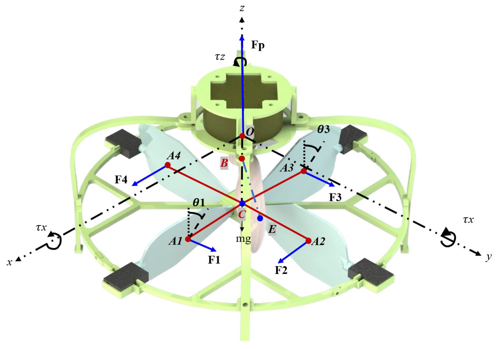
Funding

This research received no external funding.

Data Availability Statement

Data sharing is not applicable to this article.

Conflicts of Interest

The authors declare no conflict of interest.

Abbreviations

The following abbreviations are used in this manuscript:
( ) B f Body frame
ω B f Angular velocity of the center of mass of the UAV
υ B f Velocity of the center of mass of the UAV
[ ϕ ¨ , θ ¨ , ψ ¨ ]           Angular acceleration vector
[ x ¨ , y ¨ , z ¨ ] Linear accelerations
[ ϕ , θ , ψ ] Roll, pitch, and yaw angles
A M Angles mixer
A o A Angle of attack
A S M Adaptive Sliding Mode
BDrag coefficient
cCosine
c 1 , c 2 Engine parameters
D O F Degrees of freedom
eError
ϵ u , ϵ v , ϵ w Wind deviations determined by the Von Karman wind turbulence model
F B Sum of the forces acting on the UAV
hArea of the SR-UAV
JInertia matrix
K f o r c e Maximum force generated by the propeller
λ Constant
mMass of the UAV
NSize swarm
N d Number of dimensions
N i t e r Number of iterations
O = [ x , y , x ] T Is the position of the UAV center of mass (i.f.)
P u , P v , P w Noise signals
p a Particle
P I D Proportional Integral Derivative
P P I Proportional–proportional integral
P S O Particle Swarm Optimization
r n d ( ) A random number
R B I The rotation matrix
R G Matrix of gravity
[ ρ ] Air density
R M S E Root Mean Square Error
[ η ¯ I f ] Mean wind velocity
[ ξ x , y , z ] External disturbances in the form of turbulent wind gusts
[ η I f ] Wind velocity in the inertial frame
sSine
S R Single rotor
T B Sum of the moments of those forces at the center of mass
U A V Unmanned aerial vehicle
uMotor´s input
vVelocity of the particle p a
V T O L Vertical take-off and landing
wInertial weight
x b e s t Best position found by the particle
x W b e s t Best position found of the entire swarm
( X 0 , Y 0 , Z 0 ) Body frame x , y , z
( X 1 , Y 1 , Z 1 ) Inertial Frame x , y , z
i . f Inertial frame

References

  1. Alexis, K.; Nikolakopoulos, G.; Tzes, A. Model predictive control scheme for the autonomous flight of an unmanned quadrotor. In Proceedings of the 2011 IEEE International Symposium on Industrial Electronics, Gdansk, Poland, 27–30 June 2011; pp. 2243–2248. [Google Scholar]
  2. Mohsan, S.A.H.; Khan, M.A.; Noor, F.; Ullah, I.; Alsharif, M.H. Towards the unmanned aerial vehicles (UAVs): A comprehensive review. Drones 2022, 6, 147. [Google Scholar] [CrossRef]
  3. Singhal, G.; Bansod, B.; Mathew, L. Unmanned aerial vehicle classification, applications and challenges: A review. Preprints 2018, 2018110601. [Google Scholar] [CrossRef]
  4. Carholt, O.; Fresk, E.; Andrikopoulos, G.; Nikolakopoulos, G. Design, modelling and control of a single rotor UAV. In Proceedings of the 2016 24th Mediterranean Conference on Control and Automation (MED), Athens, Greece, 21–24 June 2016; pp. 840–845. [Google Scholar]
  5. Hu, Y.; Yang, Y.; Li, S.; Zhou, Y. Fuzzy controller design of micro-unmanned helicopter relying on improved genetic optimization algorithm. Aerosp. Sci. Technol. 2020, 98, 105685. [Google Scholar] [CrossRef]
  6. Shen, S.; Xu, J. Adaptive neural network-based active disturbance rejection flight control of an unmanned helicopter. Aerosp. Sci. Technol. 2021, 119, 107062. [Google Scholar] [CrossRef]
  7. Moon, J.S.; Kim, C.; Youm, Y.; Bae, J. UNI-Copter: A portable single-rotor-powered spherical unmanned aerial vehicle (UAV) with an easy-to-assemble and flexible structure. J. Mech. Sci. Technol. 2018, 32, 2289–2298. [Google Scholar] [CrossRef]
  8. Bautista-Medina, J.A.; Lozano, R.; Osorio-Cordero, A. Modeling and Control of a Single Rotor Composed of Two Fixed Wing Airplanes. Drones 2021, 5, 92. [Google Scholar] [CrossRef]
  9. Qi, X.; Qi, J.; Theilliol, D.; Zhang, Y.; Han, J.; Song, D.; Hua, C. A review on fault diagnosis and fault tolerant control methods for single-rotor aerial vehicles. J. Intell. Robot. Syst. 2014, 73, 535–555. [Google Scholar] [CrossRef]
  10. Rubí, B.; Pérez, R.; Morcego, B. A survey of path following control strategies for UAVs focused on quadrotors. J. Intell. Robot. Syst. 2020, 98, 241–265. [Google Scholar] [CrossRef]
  11. Susanto, T.; Setiawan, M.B.; Jayadi, A.; Rossi, F.; Hamdhi, A.; Sembiring, J.P. Application of Unmanned Aircraft PID Control System for Roll, Pitch and Yaw Stability on Fixed Wings. In Proceedings of the 2021 International Conference on Computer Science, Information Technology, and Electrical Engineering (ICOMITEE), Banyuwangi, Indonesia, 27–28 October 2021; pp. 186–190. [Google Scholar]
  12. Zhang, B.; Zhang, W.; Mou, J.; Yang, R.; Zhang, Y. Fuzzy PID Controller for UAV Based on Reinforcement Learning. In Proceedings of the 2022 International Conference on Autonomous Unmanned Systems (ICAUS 2022), Xi’an, China, 23–25 September 2023; pp. 1724–1732. [Google Scholar]
  13. Kahouadji, M.; Mokhtari, M.R.; Choukchou-Braham, A.; Cherki, B. Real-time attitude control of 3 DOF quadrotor UAV using modified super twisting algorithm. J. Frankl. Inst. 2020, 357, 2681–2695. [Google Scholar] [CrossRef]
  14. Lee, D.; Jin Kim, H.; Sastry, S. Feedback linearization vs. adaptive sliding mode control for a quadrotor helicopter. Int. J. Control. Autom. Syst. 2009, 7, 419–428. [Google Scholar] [CrossRef]
  15. Swikir, A.; Utkin, V. Chattering analysis of conventional and super twisting sliding mode control algorithm. In Proceedings of the 2016 14th International Workshop on Variable Structure Systems (VSS), Nanjing, China, 1–4 June 2016; pp. 98–102. [Google Scholar]
  16. Srinivasarao, G.; Arun, K.; Samantaray, S.K.G. Cascaded adaptive integral backstepping sliding mode and super-twisting controller for twin rotor system using bond graph model. ISA Trans. 2022, 1, 516–532. [Google Scholar] [CrossRef] [PubMed]
  17. Sanwale, J.; Dahiya, S.; Trivedi, P.; Kothari, M. Robust fault-tolerant adaptive integral dynamic sliding mode control using finite-time disturbance observer for coaxial octorotor UAVs. Control. Eng. Pract. 2023, 1, 1–14. [Google Scholar] [CrossRef]
  18. Ricardo, J.A., Jr.; Santos, D.A. Smooth second-order sliding mode control for fully actuated multirotor aerial vehicles. ISA Trans. 2022, 1, 169–178. [Google Scholar] [CrossRef]
  19. Serrano, F.; Castillo, O.; Alassafi, M.; Alsaadi, F.; Ahmad, A. Terminal sliding mode attitude-position quaternion based control of quadrotor unmanned aerial vehicle. Adv. Space Res. 2023, 1, 3855–3867. [Google Scholar] [CrossRef]
  20. Mofid, O.; Mobayen, S. Adaptive sliding mode control for finite-time stability of quad-rotor UAVs with parametric uncertainties. ISA Trans. 2018, 72, 1–14. [Google Scholar] [CrossRef]
  21. Huang, T.; Huang, D.; Wang, Z.; Shah, A. Robust tracking control of a quadrotor UAV based on adaptive sliding mode controller. Complexity 2019, 2019, 7931632. [Google Scholar] [CrossRef]
  22. Eltayeb, A.; Rahmat, M.F.; Basri, M.A.M.; Eltoum, M.M.; El-Ferik, S. An improved design of an adaptive sliding mode controller for chattering attenuation and trajectory tracking of the quadcopter UAV. IEEE Access 2020, 8, 205968–205979. [Google Scholar] [CrossRef]
  23. Zhen, Z.; Tao, G.; Xu, Y.; Song, G. Multivariable adaptive control based consensus flight control system for UAVs formation. Aerosp. Sci. Technol. 2019, 93, 105336. [Google Scholar] [CrossRef]
  24. Altan, A.; Aslan, Ö.; Hacıoğlu, R. Model reference adaptive control of load transporting system on unmanned aerial vehicle. In Proceedings of the 2018 6th International Conference on Control Engineering & Information Technology (CEIT), Istanbul, Turkey,, 25–27 October 2018; pp. 1–5. [Google Scholar]
  25. Bianchi, D.; Di Gennaro, S.; Di Ferdinando, M.; Acosta Lùa, C. Robust Control of UAV with Disturbances and Uncertainty Estimation. Machines 2023, 11, 352. [Google Scholar] [CrossRef]
  26. Wang, B.H.; Wang, D.B.; Ali, Z.A.; Ting Ting, B.; Wang, H. An overview of various kinds of wind effects on unmanned aerial vehicle. Meas. Control 2019, 52, 731–739. [Google Scholar] [CrossRef]
  27. Kennedy, J.; Eberhart, R. Particle swarm optimization. In Proceedings of the ICNN’95-International Conference on Neural Networks, Perth, WA, Australia, 27 November–1 December 1995; Volume 4, pp. 1942–1948. [Google Scholar]
  28. Marini, F.; Walczak, B. Particle swarm optimization (PSO). A tutorial. Chemom. Intell. Lab. Syst. 2015, 149, 153–165. [Google Scholar] [CrossRef]
  29. Kachitvichyanukul, V. Comparison of three evolutionary algorithms: GA, PSO, and DE. Ind. Eng. Manag. Syst. 2012, 11, 215–223. [Google Scholar] [CrossRef]
  30. Rajesh, R.; Ananda, C. PSO tuned PID controller for controlling camera position in UAV using 2-axis gimbal. In Proceedings of the 2015 International Conference on Power and Advanced Control Engineering (ICPACE), Bengaluru, India, 12–14 August 2015; pp. 128–133. [Google Scholar]
  31. Mac, T.T.; Copot, C.; Duc, T.T.; De Keyser, R.A.R. Drone UAV control parameters tuning based on particle swarm optimization algorithm. In Proceedings of the 2016 IEEE International Conference on Automation, Quality and Testing, Robotics (AQTR), Bengaluru, India, 12–14 August 2016; pp. 1–6. [Google Scholar]
  32. Jing, X.; Wang, X. PSO algorithm tuning PI_ PID controller parameters of quad-rotor UAV. J. Phys. Conf. Ser. 2022, 2228, 012017. [Google Scholar] [CrossRef]
  33. Rendón, M.A.; Martins, F.F. Unmanned quadrotor path following nonlinear control tuning using particle swarm optimization. In Proceedings of the 2018 Latin American Robotic Symposium, 2018 Brazilian Symposium on Robotics (SBR) and 2018 Workshop on Robotics in Education (WRE), Joao Pessoa, Brazil, 6–10 November 2018; pp. 509–514. [Google Scholar]
  34. Khatiwada, S.; McCormack, J.; Thein, M.W. Particle swarm optimization tuning of fault tolerant sliding mode control for quadrotor. In Proceedings of the Dynamic Systems and Control Conference, American Society of Mechanical Engineers, Atlanta, GA, USA, 30 September–3 October 2018; Volume 51913, p. V003T37A003. [Google Scholar]
  35. Bélanger, J.; Venne, P.; Paquin, J.N. The what, where and why of real-time simulation. Planet Rt 2010, 1, 25–29. [Google Scholar]
  36. Dalamagkidis, K. Handbook of Unmanned Aerial Vehicles; Valavanis, K.P., Vachtsevan, G.J., Eds.; Springer: Berlin/Heidelberg, Germany, 2015; p. 44. [Google Scholar]
  37. Feng, Y.; Zhou, M.; Han, Q.L.; Han, F.; Cao, Z.; Ding, S. Integral-type sliding-mode control for a class of mechatronic systems with gain adaptation. IEEE Trans. Ind. Inform. 2019, 16, 5357–5368. [Google Scholar] [CrossRef]
  38. Stroe, G.; Andrei, I.C. Analysis Regarding the Effects of Atmospheric Turbulence on Aircraft Dynamics. INCAS Bull. 2016, 8, 123. [Google Scholar]
  39. Puig-Navarro, J.; Ackerman, K.; Hovakimyan, N.; Cotting, M.C.; Duke, D.J.; Carrera, M.J.; McCaskey, N.C.; Esposito, D.; Peterson, J.M.; Tellefsen, J.R. An L1 adaptive stability augmentation system designed for MIL-HDBK-1797 level 1 flying qualities. In Proceedings of the AIAA SciTech 2019 Forum, San Diego, CA, USA, 7–11 January 2019; p. 1083. [Google Scholar]
  40. Liu, X.; Abà, A.; Capone, P.; Manfriani, L.; Fu, Y. Atmospheric Disturbance Modelling for a Piloted Flight Simulation Study of Airplane Safety Envelope over Complex Terrain. Aerospace 2022, 9, 103. [Google Scholar] [CrossRef]
  41. Åström, K.J.; Hägglund, T. The future of PID control. IFAC Proc. Vol. 2000, 33, 19–30. [Google Scholar] [CrossRef]
  42. Salih, A.L.; Moghavvemi, M.; Mohamed, H.A.; Gaeid, K.S. Flight PID controller design for a UAV quadrotor. Sci. Res. Essays 2010, 5, 3660–3667. [Google Scholar]
  43. Rao, P.G.K.; Subramanyam, M.; Satyaprasad, K. Study on PID controller design and performance based on tuning techniques. In Proceedings of the 2014 International Conference on Control, Instrumentation, Communication and Computational Technologies (ICCICCT), Kanyakumari, India, 10–11 July 2014; pp. 1411–1417. [Google Scholar]
  44. Shtessel, Y.; Edwards, C.; Fridman, L.; Levant, A. Sliding Mode Control and Observation; Springer: Berlin/Heidelberg, Germany, 2014; Volume 10. [Google Scholar]
  45. Levant, A. Sliding order and sliding accuracy in sliding mode control. Int. J. Control 1993, 58, 1247–1263. [Google Scholar] [CrossRef]
  46. Castañeda, H.; Salas-Peña, O.S.; de León-Morales, J. Extended observer based on adaptive second order sliding mode control for a fixed wing UAV. ISA Trans. 2017, 66, 226–232. [Google Scholar] [CrossRef]
  47. Baek, J.; Kwon, W. Practical adaptive sliding-mode control approach for precise tracking of robot manipulators. Appl. Sci. 2020, 10, 2909. [Google Scholar] [CrossRef]
  48. Castañeda, H.; Rodriguez, J.; Gordillo, J.L. Continuous and smooth differentiator based on adaptive sliding mode control for a quad-rotor MAV. Asian J. Control 2021, 23, 661–672. [Google Scholar] [CrossRef]
  49. Plestan, F.; Shtessel, Y.; Bregeault, V.; Poznyak, A. New methodologies for adaptive sliding mode control. Int. J. Control. 2010, 83, 1907–1919. [Google Scholar] [CrossRef]
  50. Schwaab, M.; Biscaia, E.C., Jr.; Monteiro, J.L.; Pinto, J.C. Nonlinear parameter estimation through particle swarm optimization. Chem. Eng. Sci. 2008, 63, 1542–1552. [Google Scholar] [CrossRef]
  51. Chu, H.J.; Chang, L.C. Applying particle swarm optimization to parameter estimation of the nonlinear Muskingum model. J. Hydrol. Eng. 2009, 14, 1024–1027. [Google Scholar] [CrossRef]
  52. Zhang, Q.L.; Li, X.; Tran, Q.A. A modified particle swarm optimization algorithm. In Proceedings of the 2005 International Conference on Machine Learning and Cybernetics, Guangzhou, China, 18–21 August 2005; Volume 5, pp. 2993–2995. [Google Scholar]
  53. Clerc, M. The swarm and the queen: Towards a deterministic and adaptive particle swarm optimization. In Proceedings of the Proceedings of the 1999 Congress on Evolutionary Computation-CEC99 (Cat. No. 99TH8406), Washington, DC, USA, 6–9 July 1999; Volume 3, pp. 1951–1957. [Google Scholar]
  54. Solihin, M.; Tack, L.; Moey, L.K. Tuning of PID Controller Using Particle Swarm Optimization (PSO). In Proceedings of the International Conference on Advanced Science, Engineering and Information Technology, Seoul, Republic of Korea, 27–29 September 2011. [Google Scholar]
  55. Nayeem, G.M.; Fan, M.; Akhter, Y. A time-varying adaptive inertia weight based modified PSO algorithm for UAV path planning. In Proceedings of the 2021 2nd International Conference on Robotics, Electrical and Signal Processing Techniques (ICREST), Khaka, Bangladesh, 5–7 January 2021; pp. 573–576. [Google Scholar]
  56. Chehadeh, M.S.; Boiko, I. Design of rules for in-flight non-parametric tuning of PID controllers for unmanned aerial vehicles. J. Frankl. Inst. 2019, 356, 474–491. [Google Scholar] [CrossRef]
  57. Karunasingha, D.S.K. Root mean square error or mean absolute error? Use their ratio as well. Inf. Sci. 2022, 585, 609–629. [Google Scholar] [CrossRef]
  58. Ju, C.; Son, H.I. Multiple UAV systems for agricultural applications: Control, implementation, and evaluation. Electronics 2018, 7, 162. [Google Scholar] [CrossRef]
Figure 1. Acting force diagram of the SR-UAV body frame.
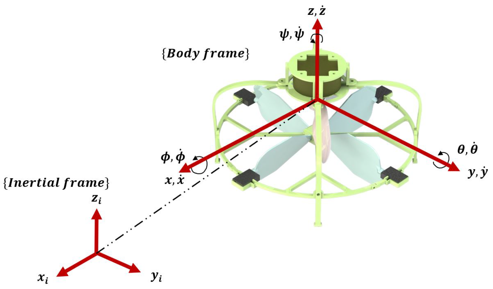
Machines 11 00870 g001
Figure 2. Inertial and body frame of the SR-UAV.
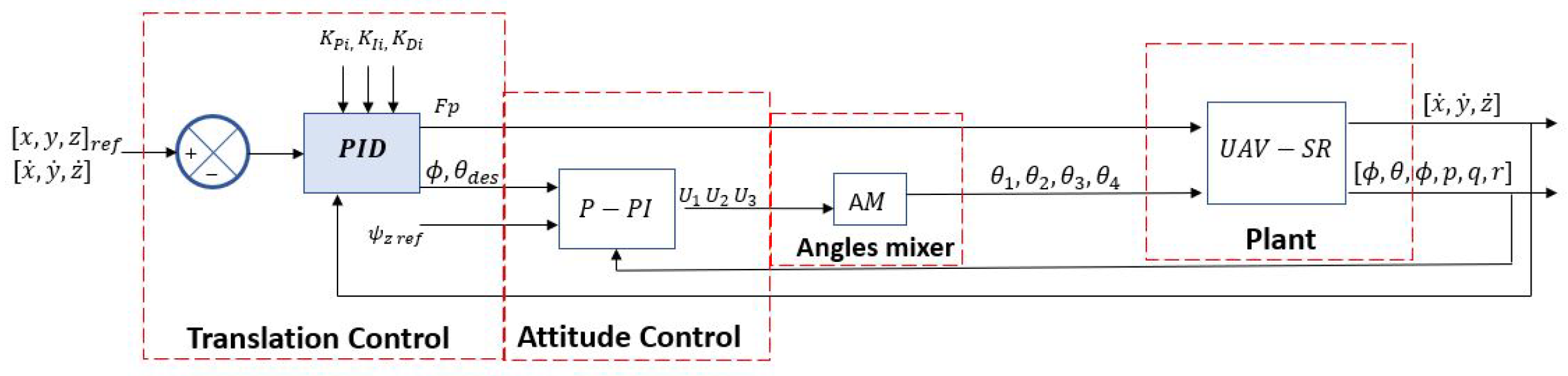
Machines 11 00870 g002
Figure 3. PID in cascade with a P-PI for translation and attitude control.
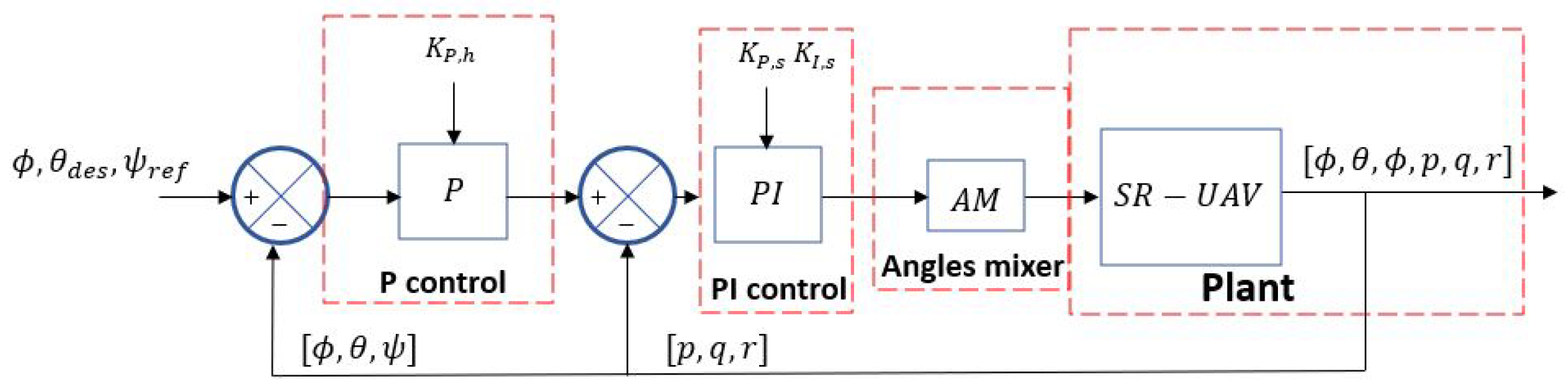
Machines 11 00870 g003
Figure 4. P-PI attitude control.
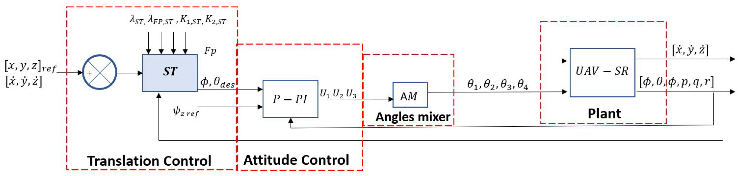
Machines 11 00870 g004
Figure 5. SR-UAV system control, where Super-Twisting method is used for translational control.
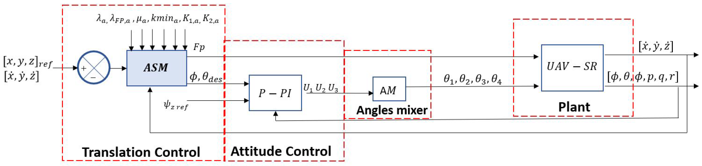
Machines 11 00870 g005
Figure 6. SR-UAV system control, where Adaptive Sliding Mode method is used for translational control.
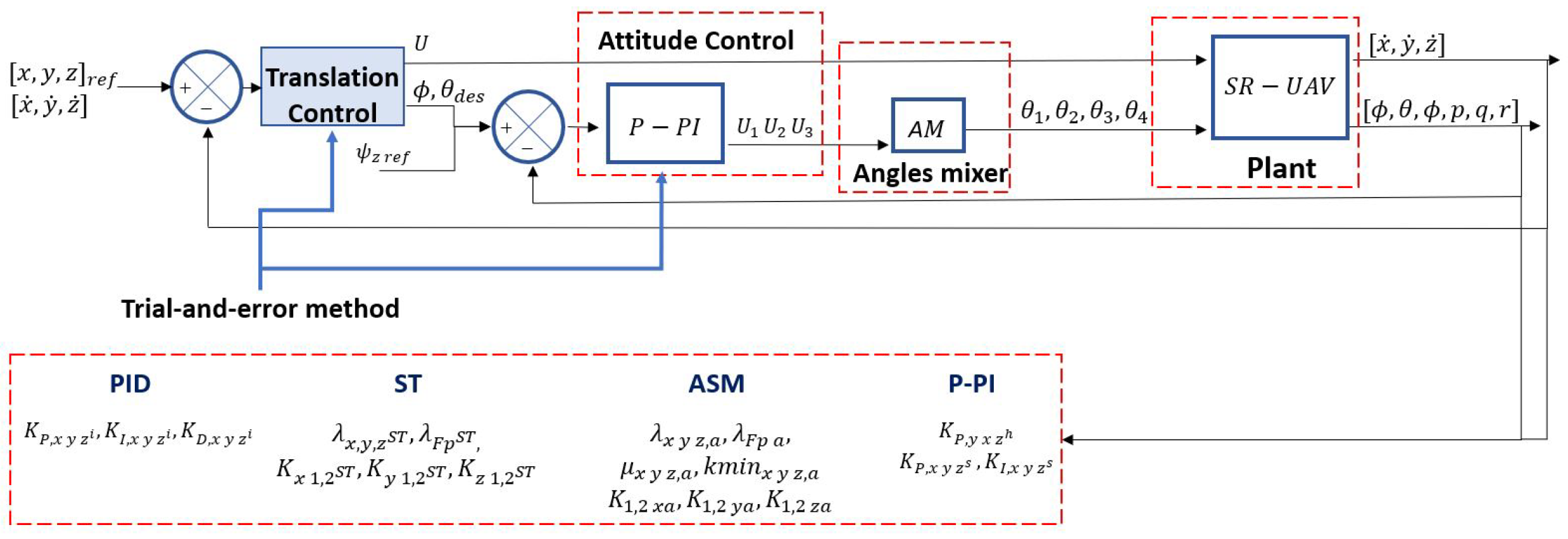
Machines 11 00870 g006
Figure 7. Control scheme with the trial-and-error method.
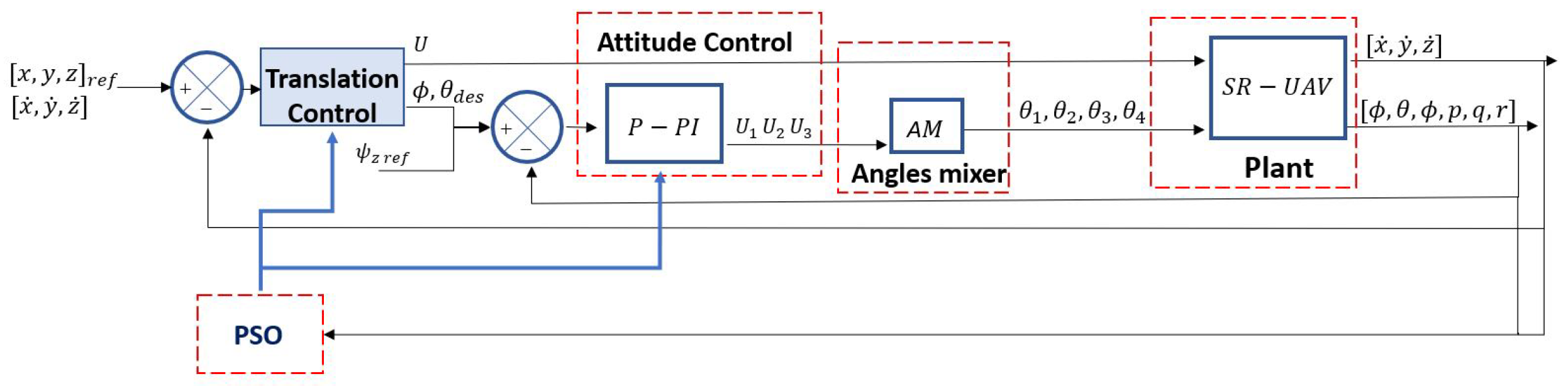
Machines 11 00870 g007
Figure 8. Control scheme with the PSO method.
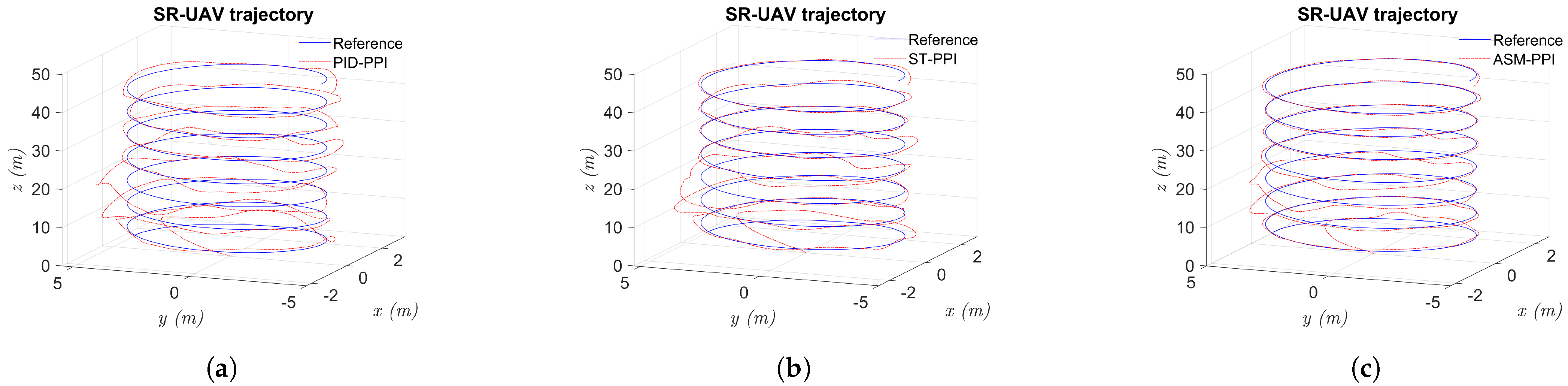
Machines 11 00870 g008
Figure 9. Helicoidal trajectory for PID, ST, and ASM with trial-and-error tuning compared with reference path. (a) Controller PID-PPI with a helicoidal trajectory. (b) Controller ST-PPI with a helicoidal trajectory. (c) Controller ASM-PPI with a helicoidal trajectory.
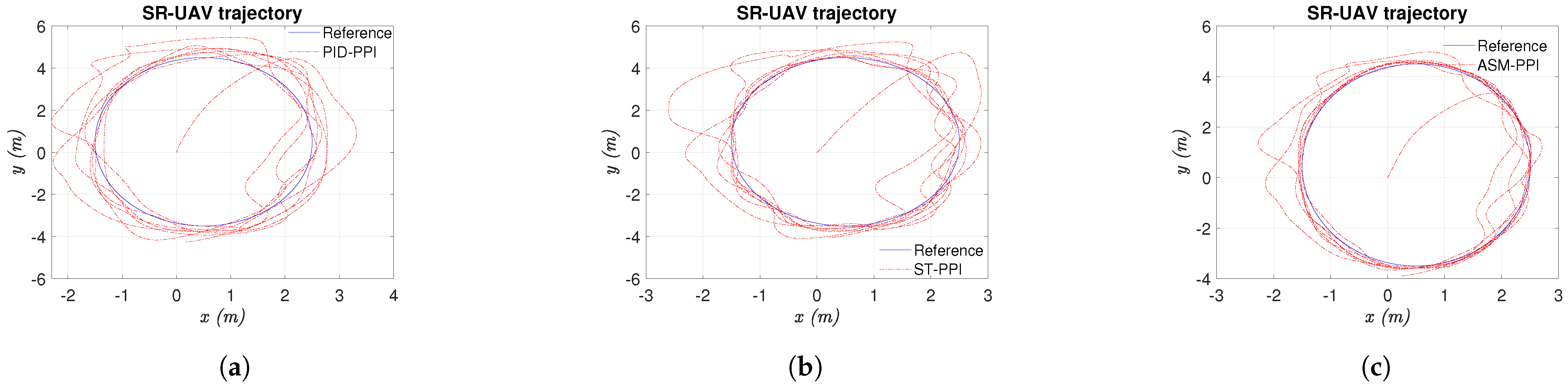
Machines 11 00870 g009
Figure 10. Helicoidal trajectory for PID, ST, and ASM in 2D compared with trial-and-error tuning. (a) Controller PID-PPI with a helicoidal trajectory in 2D. (b) Controller ST-PPI with a helicoidal trajectory in 2D. (c) Controller ASM-PPI with a helicoidal trajectory in 2D.
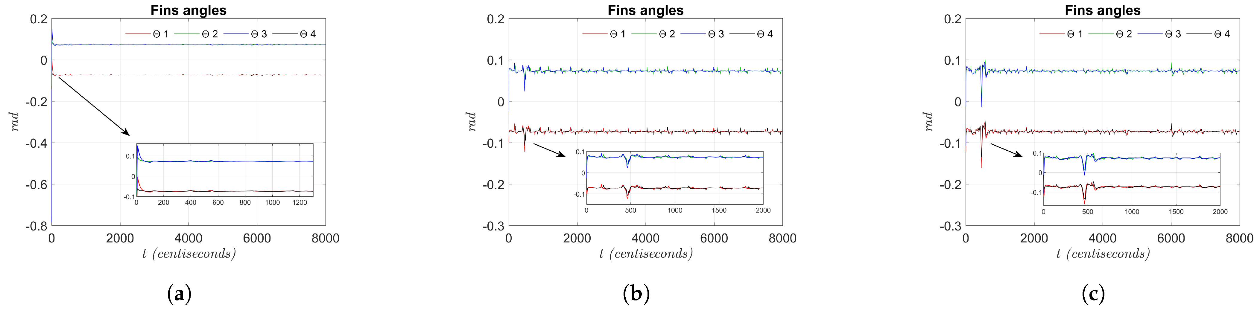
Machines 11 00870 g010
Figure 11. Servomotor fin angles for PID, ST, and ASM. (a) Angles of PID-PPI with a helicoidal trajectory. (b) Angles of ST-PPI with a helicoidal trajectory. (c) Angles of ASM-PPI with a helicoidal trajectory.
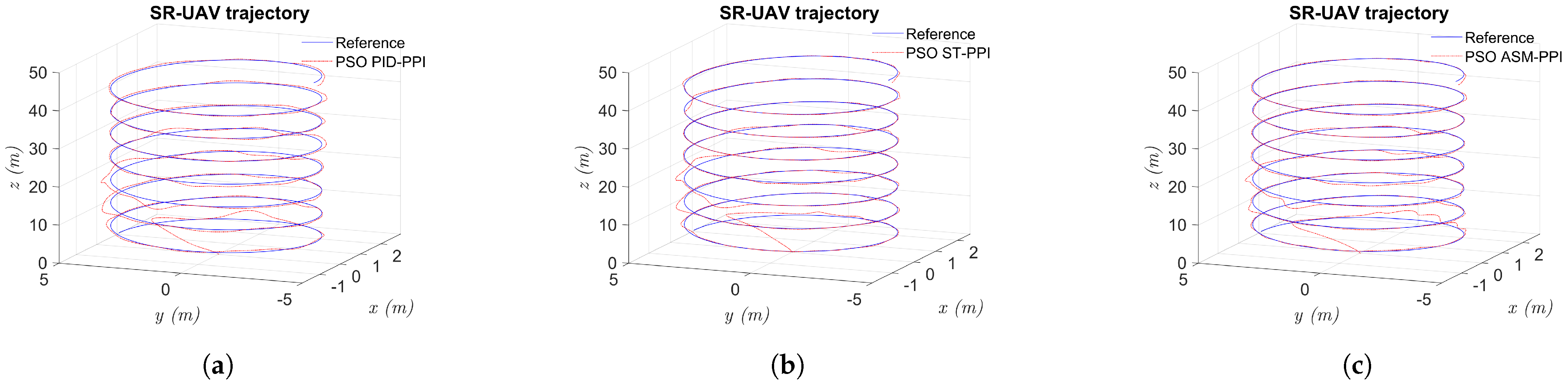
Machines 11 00870 g011
Figure 12. Helicoidal trajectory for PID, ST, and ASM tuned with PSO and compared with reference path. (a) Controller PID-PPI with PSO gains. (b) Controller ST-PPI with PSO gains. (c) Controller ASM-PPI with PSO gains.
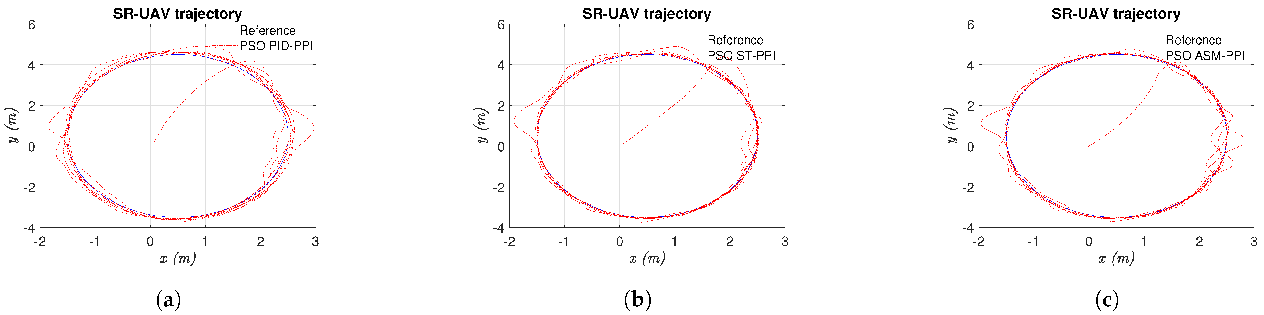
Machines 11 00870 g012
Figure 13. Helicoidal trajectory for PID, ST, and ASM with PSO in 2D. (a) Controller PID-PPI with PSO gains in 2D. (b) Controller ST-PPI with PSO gains in 2D. (c) Controller ASM-PPI with PSO gains in 2D.
Machines 11 00870 g013
Figure 14. Servomotor fin angles for PID, ST, and ASM. (a) Angles of controller PID-PPI with PSO. (b) Angles of controller ST-PPI with PSO. (c) Angles of controller ASM-PPI with PSO.
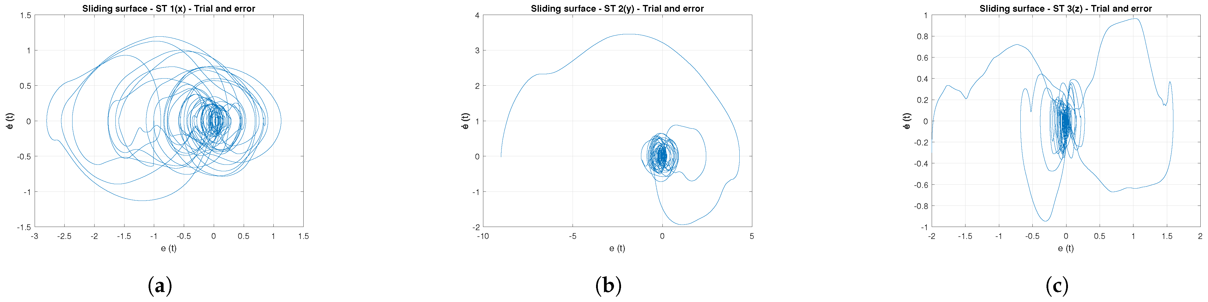
Machines 11 00870 g014
Figure 15. Sliding surface for ST with trial-and-error. (a) Sliding surface—ST 1(x)—trial and error. (b) Sliding surface—ST 2(y)—trial and error. (c) Sliding surface—ST 3(z)—trial and error.
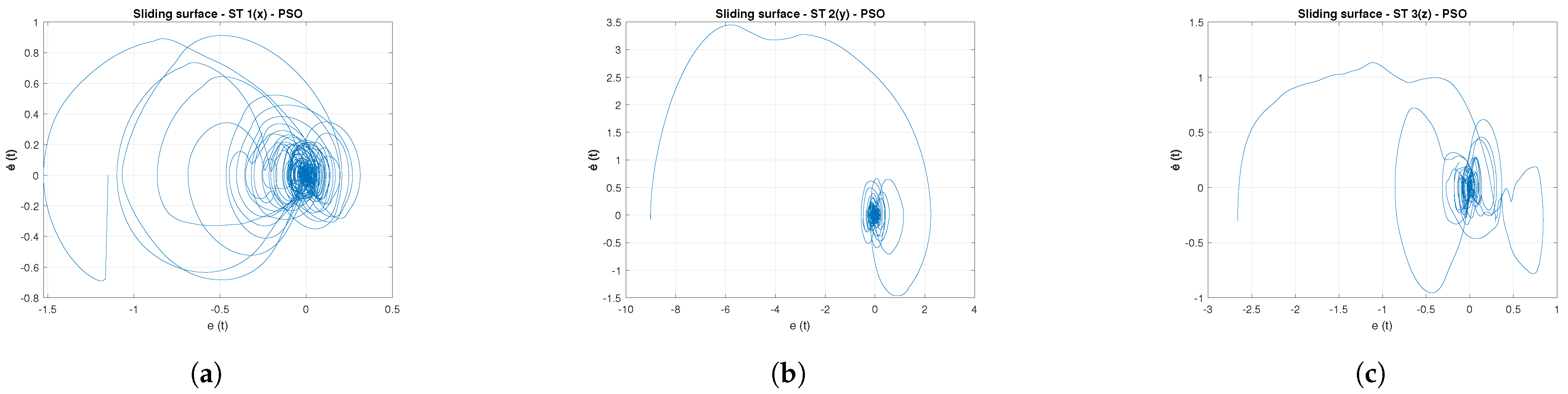
Machines 11 00870 g015
Figure 16. Sliding surface for ST with PSO. (a) Sliding surface—ST 1(x)—PSO. (b) Sliding surface—ST 2(y)—PSO. (c) Sliding surface—ST 3(z)—PSO.
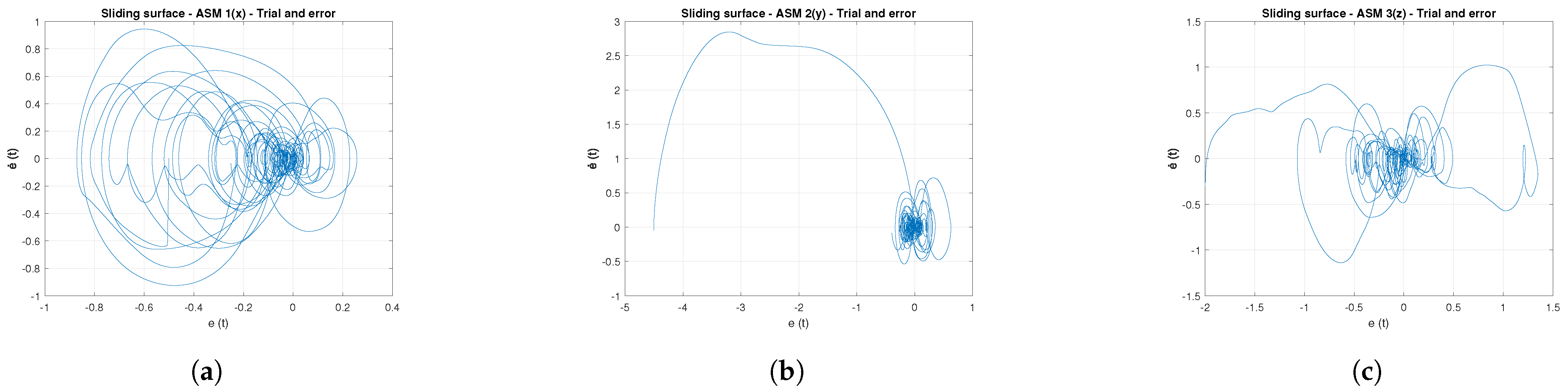
Machines 11 00870 g016
Figure 17. Sliding surface for ASM with trial and error. (a) Sliding surface—ASM 1(x)—trial and error. (b) Sliding surface—ASM 2(y)—trial and error. (c) Sliding surface—ASM 3(z)—trial and error.
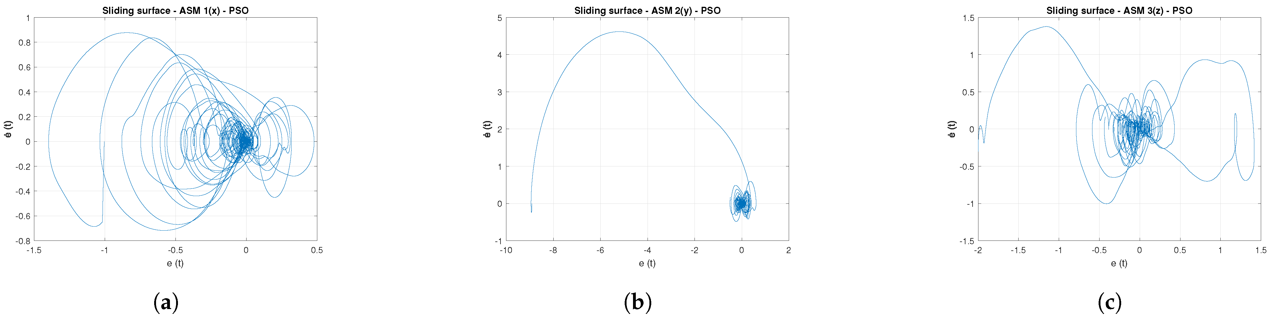
Machines 11 00870 g017
Figure 18. Sliding surface for ASM with PSO. (a) Sliding surface—ASM 1(x)—PSO. (b) Sliding surface—ASM 2(y)—PSO. (c) Sliding surface—ASM 3(z)—PSO.
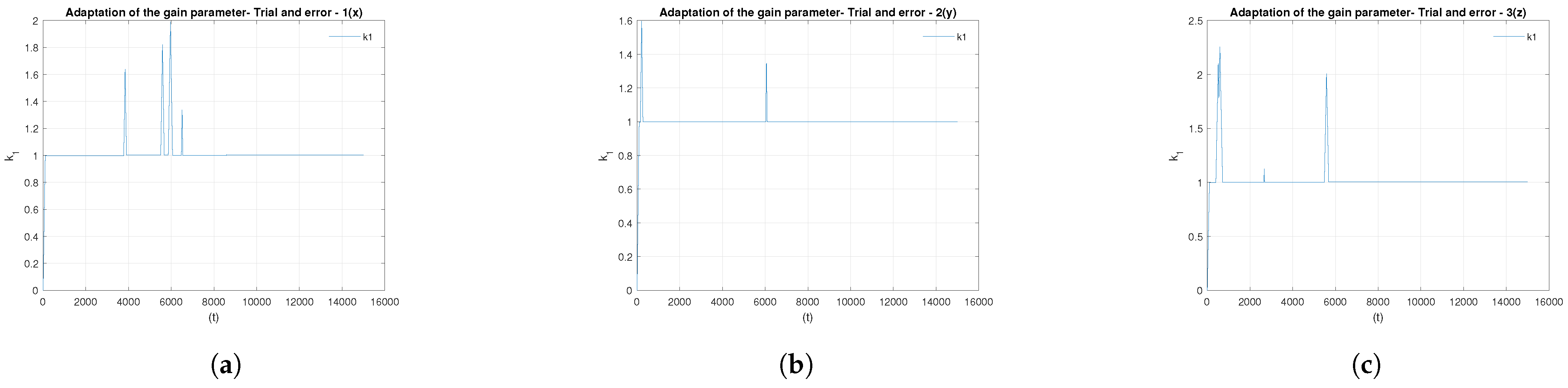
Machines 11 00870 g018
Figure 19. Adaptation of the gain parameter for ASM with trial-and-error method. (a) Adaptation of the gain parameter—trial and error—1(x). (b) Adaptation of the gain parameter—trial and error—2(y). (c) Adaptation of the gain parameter—trial and error—3(z).
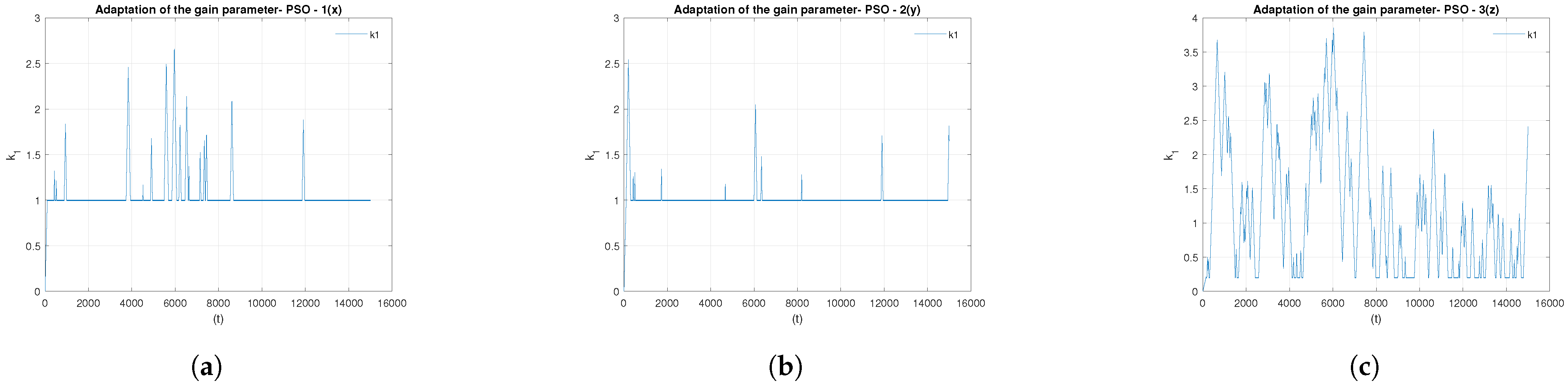
Machines 11 00870 g019
Figure 20. Adaptation of the gain parameter for ASM with PSO. (a) Adaptation of the gain parameter—PSO—1(x). (b) Adaptation of the gain parameter—PSO—2(y). (c) Adaptation of the gain parameter—PSO—3(z).
Machines 11 00870 g020
Table 1. PID, Super Twisting, and Adaptive Sliding Mode parameters and gains.
PIDSuper TwistingAdaptive Sliding Mode
Translation CAttitude CTranslation CAttitude CTranslation CAttitude C
K P , x i K P , x h λ x S T K P , x h λ x a K P , x h
K P , y i K P , y h λ y S T K P , y h λ y a K P , y h
K P , z i K P , z h λ z S T K P , z h λ z a K P , z h
K I , x i K P , x s λ F p S T K P , x s μ x a K P , x s
K I , y i K P , y s K 1 , x S T K P , y s μ y a K P , y s
K I , z i K P , z s K 1 , y S T K P , z s μ z a K P , z s
K D , x i K I , x s K 1 , z S T K I , x s k m i n x a K I , x s
K D , y i K I , y s K 2 , x S T K I , y s k m i n y a K I , y s
K D , z i K I , z s K 2 , y S T K I , z s k m i n z a K I , z s
-- K 2 , z S T - K 1 , x a -
---- K 1 , y a -
---- K 1 , z a -
---- K 2 , x a -
---- K 2 , y a -
---- K 2 , z a -
Table 2. Parameters of the SR-UAV.
ParametersValues
m 0.393 Kg
J x x , J y y 0.0037 Kgm 2
J z z 0.0021 Kgm 2
B x , B y 0.3
B z 0.5
h x , h y 0.1 m 2
h z 0.2 m 2
L 0.106 m
r 0.084 m
K t 0.5 Nm
K f o r c e 15 N
Table 3. PID controller gains with trial-and-error tuning.
ParametersValues
K P , x i , K P , y i 1.2
K I , x i , K I , y i 0.03
K D , x i , K D , y i 0.75
K P , z i 2.1
K I , z i 0.03
K D , z i 0.6
Table 4. P-PI controller gains with trial-and-error tuning.
ParametersValues
K P , x h , K P , y h , K P , z h 7
K P , x s , K P , y s 0.3
K P , z s 0.1
K I , x s , K I , y s 0.012
K I , z s 0.003
Table 5. Parameters for ST controller.
ParametersValues
λ x S T , λ y S T , λ F p S T 2
λ z S T 1
Table 6. Gains for the ST controller with trial-and-error tuning.
ParametersValues
K 1 , x S T , K 1 , y S T 1
K 2 , x S T , K 2 , y S T 0.01
K 1 , z S T , K 2 , z S T 1
Table 7. Gains for the P-PI controller with trial-and-error tuning.
ParametersValues
K P , x h , K P , y h , K P , z h 3
K P , x s , K P , y s 0.1
K I , x s , K I , y s 0.01
K P , z s 0.1
K P , z s 0.01
Table 8. Parameters for ASM controller.
ParametersValues
λ x a , λ y a 1
λ z a , λ F p a 1
μ x a , μ y a 1
μ z a 1
k m i n x , y , z a 1
Table 9. Gains for the ASM controller with trial-and-error tuning.
ParametersValues
K 1 , x a , K 1 , y a 1
K 2 , x a , K 1 , y a 1
K 1 , z a , K 2 , z a 1
Table 10. P-PI controller gains with trial-and-error tuning.
ParametersValues
K P , x h , K P , y h , K P , z h 3
K P , x s , K P , y s , K P , z s 0.1
K I , x s , K I , y s , K I , z s 0.01
Table 11. Gains for PID controller with PSO tuning.
ParametersValues
K P , x i 4
K D , x i 2.5
K P , y i 4.1
K D , y i 2.4
K P , z i 7
K D , z i 2
K I , x i , K I , y i , K I , z i 0.1
Table 12. Gains for the P-PI controller with PSO tuning.
ParametersValues
K P , x h 6.2
K P , y h 6.1
K P , z h 6.1
K P , x s 1
K P , y s 1.05
K P , z s 0.1
K I , x s , K I , y s 0.04
K I , z s , 0.001
Table 13. Parameters for ST controller.
ParametersValues
λ x S T 2
λ y S T 2.3
λ z S T 1.33
λ F p S T 1
Table 14. Parameters for ST controller.
ParametersValues
K 1 , x S T 2.5
K 2 , x S T 0.01
K 1 , y S T 1.7
K 2 , y S T 0.01
K 1 , z S T 2.5
K 2 , z S T 1.5
Table 15. Gains for the P-PI controller with PSO tuning.
ParametersValues
K P , x h 3.5
K P , y h , K P , z h 3.4
K P , x s 0.3
K P , y s 0.35
K I , x s , K I , y s 0.04
K P , z s 0.1
K P , z s 0.01
Table 16. Gains for the ASM controller with PSO tuning.
ParametersValues
λ x a 2.01
λ y a 1.98
λ z a , λ F p a 1
μ x a , μ y a 0.5
μ z a 0.1
k m i n x , y a 1
k m i n z a 0.14
Table 17. Gains for the ASM controller with PSO tuning.
ParametersValues
K 1 , x a 1.47
K 1 , y a 1.50
K 2 , x a 0.99
K 2 , y a 1.01
K 1 , z a 1
K 2 , z a 0.98
Table 18. P-PI controller gains with PSO tuning.
ParametersValues
K P , x h 6.01
K P , y h 6.11
K P , z h 5.87
K P , x s 0.10
K P , y s 0.09
K P , z s 0.099
K I , x s 0.08
K I , y s 0.04
K I , z s 0.01
Table 19. Performance indices with trial-and-error tuning.
ControllerRMSEControl Effort
| τ | z θ 1 θ 2 θ 3 θ 4
PID-PPI0.4433480.54399.00578.95379.01098.9567
ST-PPI0.1801481.37708.96018.95818.95778.9564
ASM-PPI0.1183480.93378.97438.95418.95688.9715
Table 20. Performance indices with PSO tuning.
ControllerRMSEControl Effort
| τ | z θ 1 θ 2 θ 3 θ 4
PID-PPI0.0421483.14029.43689.43869.20169.0777
ST-PPI0.0181481.96438.98299.00978.98499.0380
ASM-PPI0.0393481.41289.07539.02019.06069.0708
Disclaimer/Publisher’s Note: The statements, opinions and data contained in all publications are solely those of the individual author(s) and contributor(s) and not of MDPI and/or the editor(s). MDPI and/or the editor(s) disclaim responsibility for any injury to people or property resulting from any ideas, methods, instructions or products referred to in the content.

