Managing Delays for Realtime Error Correction and Compensation of an Industrial Robot in an Open Network

Abstract

The calibration of articulated arms presents a substantial challenge within the manufacturing domain, necessitating sophisticated calibration systems often reliant on the integration of costly metrology equipment for ensuring high precision. However, the logistical complexities and financial burden associated with deploying these devices across diverse systems hinder their widespread adoption. In response, Industry 4.0 emerges as a transformative paradigm by enabling the integration of manufacturing devices into networked environments, thereby providing access through cloud-based infrastructure. Nonetheless, this transition introduces a significant concern in the form of network-induced delays, which can significantly impact realtime calibration procedures. To address this pivotal challenge, the present study introduces an innovative framework that adeptly manages and mitigates network-induced delays. This framework leverages two key components: controller and optimiser, specifically the MPC (Model Predictive Controller) in conjunction with the Extended Kalman Filter (EKF), and a Predictor, characterised as the Dead Reckoning Model (DRM). Collectively, these methodologies are strategically integrated to address and ameliorate the temporal delays experienced during the calibration process. Significantly expanding upon antecedent investigations, the study transcends prior boundaries by implementing an advanced realtime error correction system across networked environments, with particular emphasis on the intricate management of delays originating from network traffic dynamics. The fundamental aim of this research extension is twofold: firstly, it aims to enhance realtime system performance on open networks, while concurrently achieving an impressive level of error correction precision at 0.02 mm. The employment of the proposed methodologies is anticipated to effectively surmount the intricacies and challenges associated with network-induced delays. Subsequently, this endeavour serves to catalyse accurate and efficient calibration procedures in the context of realtime manufacturing scenarios. This research significantly advances the landscape of error correction systems and lays a robust groundwork for the optimised utilisation of networked manufacturing devices within the dynamic realm of Industry 4.0 applications.

1. Introduction

Large-scale, complex, and low-volume manufacturing systems, particularly in the aerospace industry, rely heavily on robotics for automation. The precision required for tasks like position accuracy, module assembly, inspection, and fastening poses unique challenges due to robot kinematics and environmental factors. Existing packages provid-ed by robot manufacturers for error correction and compensation suffer from cost and lack of realtime capabilities, resulting in static correction and dedicated resources. The research addressed these challenges by developing a dynamic and realtime error correction system, achieving error correction in the range of 0.02 mm. [1] The study extends the existing re-search by implementing the proposed system over the network and addressing the chal-lenge of managing delays caused by network traffic.

Considering the implications of connecting the tracker or measurement device to a singular network switch, its utility is limited to a specific robotic cell as a result. In such a scenario, the tracker’s functionality would be exclusive to that particular cell, rendering it inaccessible to other cells that might require its services. The tracker’s mobility, which allows it to orient itself towards different cells as needed, would be compromised. The cost-effectiveness also comes into play when optimizing resource utilisation. Employing a single tracker for multiple cells, numbering around 10 or more, and coordinating this shared resource via a resource management system, emerges as a strategic approach. This allows the tracker’s capabilities to be harnessed across multiple cells while minimizing redundant costs. The paper could further emphasise these considerations to underscore the rationale behind the chosen network configuration.

The issue of delay represents a prominent challenge within Network Control Systems (NCS) and other systems reliant on network infrastructure. This delay stems from two primary factors: network traffic and the limited bandwidth of the communication channel. The use of Kalman filter [2,3] and MPC for NCS can help to eliminate the noise and both types of delays but still there is a need to implement a strategy to handle network delays to obtain a realtime effect in the system [4,5]. The system in question is the distributed application.

There are lots of techniques available to handle network delays for distributed Interactive applications (DIAs) [6]. Some of the techniques can be benchmarked; for example, the DRM [7] is a popular technique in positioning systems. DRM is widely used in DIA for the predictive contract agreement mechanism in managing network latencies [8]. A study shows that the use of DRM can enhance the Network speed and optimise the performance [9].

The same DRM technique can be used for NCS to predict the information about the position of the robot arm using extrapolation and the smoothing function can help to smooth the extrapolated position and real position [9,10].

MPC has also been used to deal with variable data losses and time delays in a realtime environment [4], which proves itself the most suitable method to be induced in realtime error compensation over the network. To handle delays in the NCS, the observer algorithm was proposed [11]. It proposed the two feedback loops one for the control system the other for the observer. They further used two more controllers for the anticipated and non-anticipated data. The Kalman filter [2] was proven to be useful for the environment in which data losses are common, and data are received intermittently [12]. This approach is particularly useful for a chaotic (where multiple cells are running at the same time on the network) and realtime sensitive environment (where time is crucial).

To make the system extendable, configurable, manageable, and distributed, some techniques need to be used, for example, Service Oriented Architecture (SOA) on the application level [13]. SOA is becoming popular for developing distributed and manageable manufacturing systems [14,15].

The gap here is to combine the realtime error correction with the network so the resources can be shared amongst other operations, significantly reducing cost and increasing flexibility. This study will need to deal with network issues while using the robot and measurement device connected to the network. The study will be more gelled with Industry 4.0 [16], which will be automating the error correction procedure and also allowing the resources to be shared and available over the network. The data about the resources, their scheduling, and their programs will be stored in the databases [17] which can be used as a knowledge base in the future [18].

Another study addresses compliance modeling and error compensation for an industrial robot’s application in ship hull welding [19]. The Cartesian stiffness matrix is obtained through the virtual-spring approach, a method that considers factors like actuation and structural stiffness, arm gravity, and external loads. While this approach enhances accuracy, it’s important to note that it doesn’t operate in real-time error correction on the network. The derived stiffness model offers the foundation for error compensation. This compensation method is demonstrated using an industrial robot executing a welding trajectory. The outcomes reveal that this compensation approach effectively enhances the robot’s operational accuracy. It aligns the robot’s actual trajectory, even when influenced by auxiliary loads, to closely match the intended trajectory.

In precision-demanding industrial robotic applications, a novel hybrid computational method is introduced for error compensation [20]. Combining Local POE calibration and Gaussian Process Regression, it reduces positioning errors by up to 37.2% compared to existing methods. While it proposes an innovative hybrid method for error compensation in precision industrial robotic tasks, it doesn’t address network integration or real-time adjustments, which are crucial aspects in modern manufacturing environments.

The novelty of the present study lies in addressing the intricate calibration challenges faced by articulated arms within the manufacturing domain. Traditionally, calibrating these arms necessitates costly and physically attached metrology equipment, impeding a widespread adoption due to cost and practical limitations. Leveraging Industry 4.0 principles, this study introduces an innovative approach by incorporating manufacturing devices into a networked ecosystem, thereby enabling cloud accessibility. However, the subsequent issue of network delays emerges as a significant hurdle, particularly concerning realtime calibration procedures.

To surmount this predicament, this study introduces a pioneering solution. It integrates an optimiser, the EKF, in tandem with a Predictor, the DRM. These techniques collectively combat and resolve network-induced delays encountered during calibration processes. A significant aspect of novelty lies in the integration of the DRM into the realm of robotics, with a specific focus on estimating position and error. This innovative application of DRM directly addresses the challenge associated with managing delays linked to the reception of measurements from a tracking device. By incorporating DRM, the system ensures realtime compensation by predicting and adapting to potential errors, thus enhancing the accuracy and efficiency of the compensation process. Furthermore, building upon earlier research efforts [1], this study extends the boundaries by implementing a realtime error correction system across a network. Notably, it homes in on mitigating delays stemming from network congestion.

The choice to adopt a realtime approach stems from catering to sectors characterised by a demand for substantial variability, such as shipbuilding and aircraft manufacturing. In these industries, the imperative for precision, quality, and efficiency is paramount. The offline provision of information and training, while potentially time-consuming, could lead to inefficiencies in meeting the stringent requirements of these sectors. Considering the inherent variability in components and robot paths, opting for realtime solutions becomes a pragmatic choice. The realtime approach aligns well with the need to swiftly adapt to diverse scenarios and ensure the precision demanded by these industries, making it a viable solution within this context.

This paper employs a three-section structure to systematically present its content. Section 2 comprehensively elucidates the methodology behind Realtime Error Correction over the network, encompassing aspects such as error prediction and estimation, the management of network delays, system development, and resource allocation. In Section 3, a thorough exploration of results and discussions unfolds, offering insights into the conducted tests aimed at assessing the system’s capabilities. Finally, Section 4 delves into a meticulous analysis of these findings, fostering a detailed discourse that culminates in the paper’s conclusive remarks.

2. Realtime Error Correction over the Network—Problem Realisation

The field of static Error Correction encompasses various technologies and systems, as highlighted in the Introduction. However, an unexplored area of research lies in addressing realtime error correction over regular or open networks. While the preceding section discussed systems that have been developed for realtime error correction, they lack the suitability to operate effectively over standard networks due to their stringent feedback requirements, which cannot be met within the required realtime constraints. The problem at hand encompasses several dimensions, including Realtime Error Correction on the Network, Handling Network Traffic and delays and making the resources sharable.

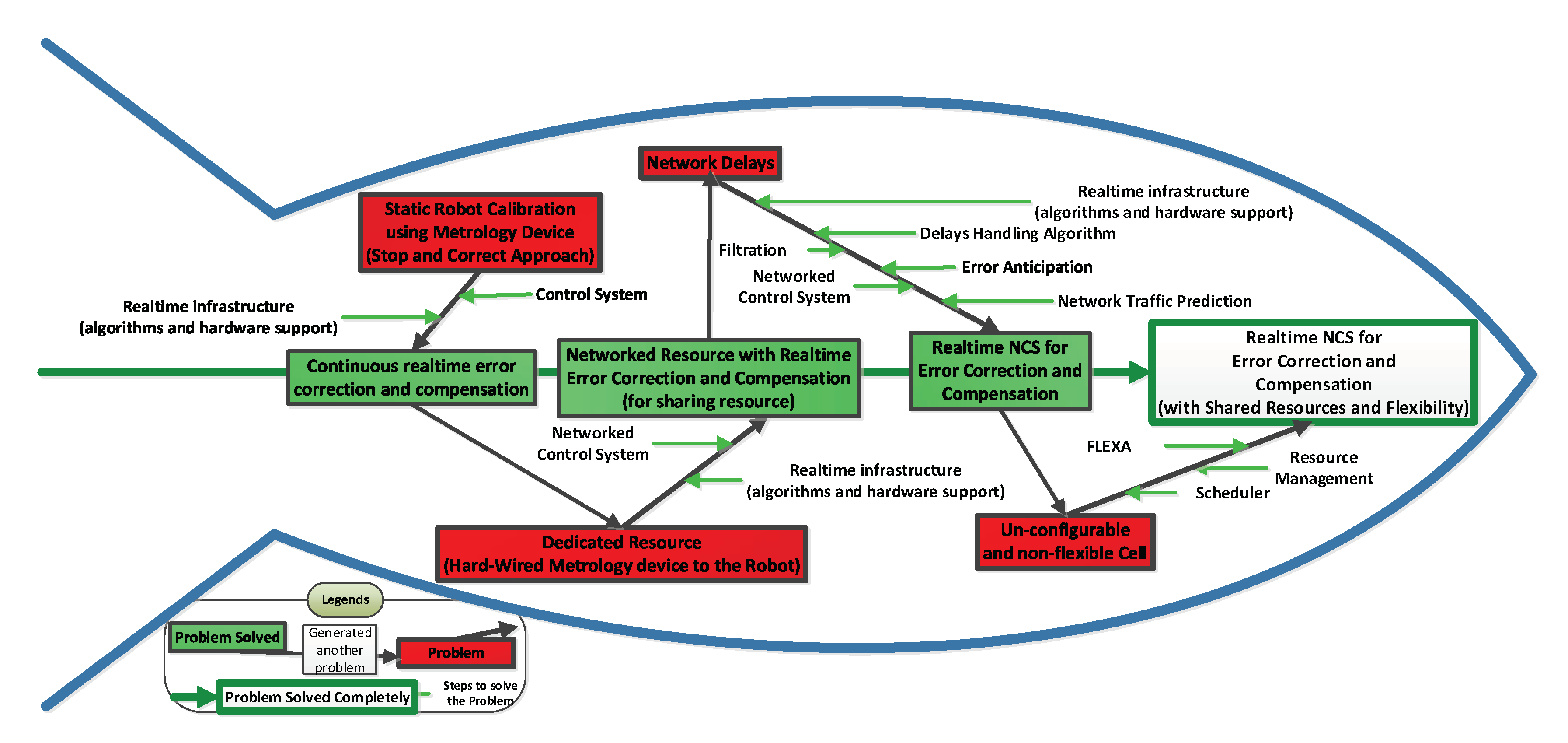
Figure 1 illustrates the resolution of the issues pertaining to static calibration and resource wastage through the implementation of a realtime networked control system, dynamic calibration techniques, and flexible resource management. The diagram visually depicts the problem area encapsulated within a red rectangle, while the corresponding solution is represented by the green region. The green arrows superimposed on the black arrows symbolise the specific approaches and algorithms employed to address the problem. The final rectangle, distinguished by a white background and a green outline, signifies the complete resolution of the problem.

The problem depicted in Figure 1 originates from the conventional static approach of Robot Calibration utilizing a metrology device. In this static approach, the error correction occurs through the Stop and Correct Approach, where the metrology device measures the position, and the system performs calculations based on these measurements. However, during this calculation period, both the system and the robot remain idle, leading to suboptimal resource utilisation and increased overall process time.

To address this issue, a feedback control system and realtime infrastructure can be employed. The realtime infrastructure encompasses hardware that supports realtime processing and the implementation of appropriate algorithms. This transforms the system into a continuous realtime error correction and compensation framework. However, this approach introduces the challenge of dedicated resources, particularly the expensive metrology equipment, which may be required by other processes on the factory shop floor.

This challenge can be overcome by incorporating a network and connecting the robot, metrology device, and other equipment to a Networked Control System, integrated with realtime infrastructure. This solution results in a Networked Resource with Realtime Error Correction and Compensation, allowing for resource sharing within this setup. Nonetheless, this approach gives rise to the problem of network delays, as the resources are interconnected over a network shared with other systems that also transmit communication data.

To mitigate network delays, various techniques can be applied, such as Filtration techniques to eliminate noise, Delay Handling Algorithms, Error Prediction (Anticipation), and Network Traffic Prediction utilising realtime infrastructure. The resulting system would be a Realtime Networked Control System for Error Correction and Compensation. However, such a system may suffer from the drawback of un-configurable and non-flexible cells.

To address the management and scheduling of resources when multiple systems and cells require the metrology device simultaneously, the Flexa Control Approach [17] can be applied. This approach integrates the Flexa Cell Controller into the system, ensuring effective resource management and scheduling.

One of the key objectives of the study is to facilitate resource sharing. In the context of automation, resources can be effectively shared through the utilisation of a network. DIA enable users to connect to the network using the same application and seamlessly share the application’s state in realtime. This synchronous sharing allows for collaborative activities such as shared whiteboarding, collaborative editing of files, joint editing of files, shared meeting rooms, and multiplayer games. Through DIA, users can interact and collaborate over a computer network, engaging in interactive work on a single application.

A fundamental characteristic of all DIAs is the shared user space and concurrent manipulation of the same data. However, the effective synchronisation and management of resources pose significant challenges for distributed applications. The issue of synchronisation becomes more complex in networked environments due to the presence of other concurrent data communications on the network. In larger networks, the system for sharing the status of each user can become time-consuming, potentially causing delays throughout the entire network. To mitigate this issue, an estimation and filtering approach can be employed to minimise the frequency of updates transmitted over the network. The DRM serves as a foundational protocol within the IEEE Standard for DIAs, particularly in the context of estimation techniques [6].

The Dead Reckoning algorithm is widely utilised in distributed network games, where the delivery of realtime experiences to users is crucial, and factors such as speed and timing play significant roles. This algorithm is derived from deduced reckoning principles and serves as an effective approach in such gaming environments.

The Dead Reckoning Algorithm utilises previous packet information, performs extrapolation to estimate future positions, and employs pre-reckoning to anticipate positions before official reckoning, reducing network packet frequency.

By employing the Dead Reckoning algorithm, fewer packets need to be transmitted over the network, leading to reduced network traffic while simultaneously improving latency. This approach enables efficient utilisation of network resources and enhances the realtime experience for users in distributed network games.

The term “dead reckoning” has a historical origin and was documented in the Oxford Dictionary in 1613. This concept involves the estimation or prediction of a future position based on knowledge of the initial starting position. When considering the concept in terms of speed, it becomes straightforward to illustrate. For instance, let us consider a hypothetical scenario where a ship sets sail at 0900 with a constant speed of 7 mph. The question then arises: Where will the ship be located along its designated course at 1100?

By applying the distance equation, the distance covered by the boat after a duration of 2 h can be calculated as 14 units. This calculation provides an estimation or reckoning of the distance travelled by the object at the specified time.

The concept of DIA has been prevalent for many years, and one of its notable examples is network games, which enable realtime gameplay over a network. DIA aims to achieve realtime interaction while maintaining robustness, reliability, security, scalability, and consistency, among other qualities. However, latency poses a significant challenge for DIA applications. Although increased bandwidth and processor speed have a positive impact on latency control, latencies still exist due to network congestion. In realtime DIAs, these latencies are deemed unacceptable. To address this, the DRM has emerged as a popular technique in positioning systems, aiding in mitigating the impact of latency [3].

The DRM has gained widespread adoption as a predictive contract agreement mechanism within DIA to effectively manage network delays [4]. A study conducted on optimising network performance utilizing DRM provides evidence that this approach can enhance overall network performance and significantly reduce latencies. The findings of the study highlight the effectiveness of DRM in addressing the challenges posed by network delays and its potential to improve the performance of DIA systems [5].

In the current problem scenario, the application of the DRM technique, in conjunction with a smoothing function, can be utilised to extrapolate and predict data and positions. DRM enables the prediction of positions between data updates. However, a potential issue arises when the predicted position does not align with the actual position obtained from the arrived data. To address this problem, a smoothing function, as suggested by [6], is employed. The smoothing function aims to reduce discontinuities by considering time compensation to compensate for packet latency. This approach helps to ensure a more seamless and accurate representation of positions within the system.

2.1. Error Prediction and Estimations for Compensating Network Delays

The fundamental principle of the system is to operate on an open network, allowing for the sharing of resources. In this context, the critical resource to be shared is the Laser Tracker, which carries a significant cost of at least £150 k. However, this requirement of the system to operate on a network introduces the challenge of managing variable network traffic.

Direct connectivity between a resource, such as a Laser Tracker, and a robot in isolation enables fast and efficient communication. However, this approach limits the resource’s usage exclusively to that particular system. The objective is to share the resource across the network, allowing other cells or systems to benefit from the error correction capabilities. Introducing the system to the network introduces the challenge of handling delays due to the presence of normal network traffic. While this may not pose a problem for static error correction, the goal is to perform a dynamic error correction [21]. In this dynamic scenario, the error correction system cannot afford to wait for measurements from the laser tracker; instead, it must ensure timely delivery to meet the realtime and dynamic demands of the system. This situation is visually depicted in Figure 2.

2.2. Dead Reckoning—Modelling (DRM)

In order to achieve realtime correction in the calibration system, it is crucial to have regular and uninterrupted feedback from the measurement system. The Dead Reckoning approach, described in previous section, provides a solution by estimating the current error using past observations. By extrapolating or predicting data values between two updates, Dead Reckoning enables the system to accommodate more connected stations and enhance the reliability of receiving measurements from the tracker. This approach improves the overall performance and robustness of the calibration system.

The calibration system is represented as a player within the overall system, operating independently from the tracker system. The term “players” is borrowed from online gaming, where Dead Reckoning is commonly used to address network delays [4,16]. Player 1 represents the tracker system, which sends updates at unpredictable intervals over the network. Player 2 represents the calibration system, which receives measurement information from the laser tracker system. The system model, depicted in Figure 3, illustrates the independent movement of the players and their periodic transmission of robot position updates.

In the system, Player 1 (Laser Tracker System) transmits the measured position of the robot, while Player 2 reports the number of the last received position. DRM is employed by Player 2 (system performing the calibration) to estimate the subsequent measured position provided by Player 1. Additionally, Player 1 utilises Dead Reckoning to track the updates it has sent and confirms that they have been properly incorporated into Player 2’s system. The network model accounts for latency, acknowledging that it takes time for updated measurements to be delivered to the other system.

2.3. System Development

System development serves as the final stage of the research, encompassing various aspects such as software modules and kinematics, which are essential for the development of the system [17]. In order to undertake this development, the following equipment was utilised: the Comau NM45 C4G robot, Leica Tracker AT901-MR along with a 3D reflector (SMR) and T-MAC for 6D measurements, the NI CRIO-9024 Realtime Controller, C# for interface development, C++ for realtime error correction and compensation module development, and LabVIEW for running the system on CRIO. These components were instrumental in facilitating the implementation and functionality of the developed system.

The interconnections between the equipment utilised in the research are depicted in Figure 4. The Comau NM45 robot is linked to the Comau C4G Controller, which serves as its controlling unit. The C4G Controller is connected to the Network Switch, with its management being handled by the NRTEC Software 600 v1.20.

The TMAC, an integral part of the robot’s End-Effector, is connected to the Leica Tracker, which tracks its position and performs measurements. The Leica Tracker is also linked to the Network Switch, enabling its management through the NRTEC Software 600 v1.20.

To enable realtime management and execution within the cell, the NRTEC Software 600 v1.20 operates on the Compact RIO realtime controller. The Compact RIO is connected to the Network Switch, facilitating access to the equipment and management by the FLEXA Cell Coordinator.

Steeplechase VLC, a software PLC employed by FLEXA, is responsible for controlling and managing the cells and their resources. It is installed on a PC and connected to the Network Switch.

For analysing the kinematics of the Comau NM45 robot and verifying the results, Spatial Analyzer software was utilised in the research.

2.4. Resource Management System—Flexa Cell Coordinator

The Flexa Cell Coordinator (FCC) is an automated system that efficiently manages the allocation and removal of resources within a Flexa Cell. It coordinates the execution of received programs on the required resources in a non-conflicting manner. Multiple cell coordinators can be run simultaneously by utilizing software Programmable Logic Controller (Soft PLC), eliminating the need for the hardwired binding of resources. The FCC receives programs in the form of recipes through web services, schedules them based on resource availability, and activates sub coordinators equipped with SoftPLC controllers to manage program execution and resource control. Data exchange between the FCC and resources is facilitated, with the FCC acting as the application manager to handle data flow. This bidirectional communication enables the FCC to accept recipe data and send back processed data.

2.5. Integration of NRTEC with FCC

The integration involves several components, including the startup of the FCC and the receipt of recipes, the generation and transmission of status reports, the scheduling and execution of scheduled recipes, and the receipt of recipes from the FCC Database (FDB). The data flow within the FCC Architecture is depicted in Figure 5, which illustrates the flow of information and interactions between the different components.

Figure 5 provides a context-level or level 0 diagram of the data flow within the FCC system. It illustrates how the FCC interacts with external entities and manages the flow of data between them. On the other hand, Figure 6 presents a detailed level 1 Data Flow Diagram, showcasing the internal components of the FCC and their respective data flows. Notably, the programs executed on the NRTEC robot are overseen and managed by the FCC Sub-Coordinator within the system [12].

2.6. Dead Reckoning Model

The DRM has been employed in this research to forecast the robot’s error when measurement data are unavailable. DRM is a widely utilised technique in various applications such as positioning systems, online gaming, and navigation. It estimates the robot’s next position by considering the previous position data. However, it is important to note that DRM is susceptible to errors since it relies on the accuracy of the measurement data obtained from sensors.

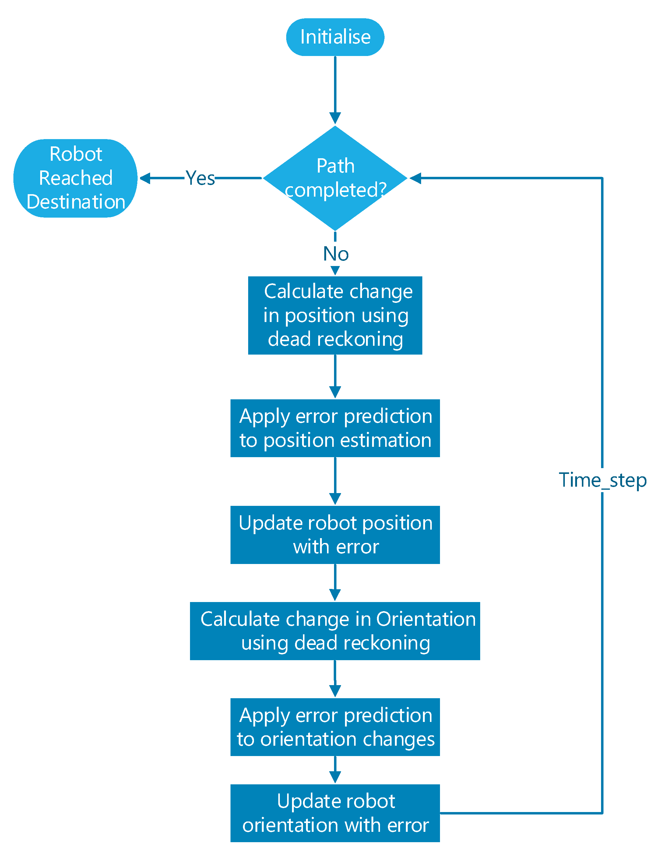
Figure 7 illustrates the design and implementation of the DRM, which incorporates a mechanism to trigger a network update if the error exceeds a predefined threshold. This approach ensures that the system responds to significant errors by requesting an update from the network, allowing for more accurate position estimation and error correction.

The changes in position are determined through the application of dead reckoning, as outlined by the equations provided below. This methodology involves estimating alterations in position based on the robot’s prior position and movement data. The equations encapsulate the relationships between the robot’s orientation and the alterations in its x, y, and z coordinates, facilitating the prediction of its updated position in response to incremental movements.

$$\Delta x=distance\_per\_step\times cos(robot\_orientation.Rz)$$

$$\Delta y=distance\_per\_step\times sin(robot\_orientation.Rz)$$

$$\Delta z=distance\_per\_step\times sin(robot\_orientation.Rx)\times cos(robot\_orientation.Rz)$$

The predicted position error is initialised randomly and computed through the utilisation of previous data and acquired error insights. Subsequently, the positions are updated by employing the predicted position error, as demonstrated by the equations provided below. This process involves integrating the anticipated error into the calculations, thereby refining the accuracy of the position updates.

$${\Delta x }_{with\_error}=\left(1+predicte{d}_{positio{n}_{error}}\right)\times \Delta x$$

$${\Delta y }_{with\_error}=\left(1+predicte{d}_{positio{n}_{error}}\right)\times \Delta y$$

$${\Delta z }_{with\_error}=\left(1+predicte{d}_{positio{n}_{error}}\right)\times \Delta z$$

Subsequently, the robot’s position requires adjustment, accounting for the introduced error. Likewise, the alteration in orientation can be computed employing dead reckoning principles, delineated by the equations presented below:

$$\Delta Rx=angle\_per\_step\times cos(robot\_orientation.Ry)\times cos(robot\_orientation.Rz)$$

$$\Delta Ry=angle\_per\_step\times cos(robot\_orientation.Rz)\times sin(robot\_orientation.Rx)$$

$$\Delta Rz=angle\_per\_step$$

Similar to the positional error, the rotational error is initialised randomly, drawing from previous data and acquired error insights. Subsequently, the rotations are refined through the incorporation of the predicted position error, as depicted by the equations provided below:

$${\Delta Rx}_{with\_error}=(1+predicted\_orientation\_error\_Rx)\times \Delta Rx$$

$${\Delta Ry}_{with\_error}=(1+predicted\_orientation\_error\_Ry)\times \Delta Ry$$

$${\Delta Rz}_{with\_error}=(1+predicted\_orientation\_error\_Rz)\times \Delta Rz$$

Figure 8 presents flowcharts that calculates the disparity between the predicted measurement and the actual measurement by using the set of above equations. The details of the pseudocode are presented in Appendix A. This enables a quantitative evaluation of the variance between the anticipated and observed values. By comparing these values, the system can assess the accuracy and precision of the prediction generated by the DRM. This evaluation is crucial for validating the effectiveness of the error correction and compensation processes within the system.

Figure 9 depicts the variation between the projected error and the actual error over the system’s progression. The graph illustrates the performance improvement of the system as it advances in time or through successive iterations. As the system evolves, the variance between the anticipated and real errors diminishes, indicating the enhanced accuracy and effectiveness of the error prediction and correction mechanisms. This graph serves as a visual representation of the system’s ability to refine its error estimation and compensation capabilities over time.

In the presented graph Figure 9, the red line represents the actual error, while the blue line represents the predicted error. Initially, the real error is observed to be around 0 and −0.1. As the system progresses through approximately 15 cycles, the predicted error gradually converges with the real error. This convergence indicates that the system successfully achieves a close alignment between the predicted error and the actual error.

2.7. EKF and MPC for the Identification of Errors

To mitigate the impact of noise and for the identification of errors, the system incorporates the use of an MPC in conjunction with an EKF. These control and filtering techniques work together to minimise the influence of noise on the error estimation and correction process. By employing the MPC and EKF, the system enhances its ability to accurately predict and compensate for errors, resulting in an improved overall performance and noise reduction.

Designing an EKF for a serial manipulator (NM45) involves defining the state vector, measurement vector, process models, noise parameters, and the overall estimation process. The state vector ‘x’ represents the robot’s pose in terms of position and orientation. For NM45, the state vector includes:

$$x=[x, y, z, Rx, Ry, Rz]’$$

The measurement vector ‘z’ includes the tracker’s measurements of the robot’s pose. The measurement vector is similar to the state vector:

$$z=[x_{measured}, y_{measured}, z_{measured}, {Rx}_{measured}, {Ry}_{measured}, {Rz}_{measured}]’$$

The state transition function, ‘f(x, u)’, or the process model, illustrates how the robot’s condition changes over time with the influence of control inputs u. These inputs are the joint velocities obtained through Jacobians that steer the robot’s movements. The specific behaviour of this function is tied to the Comau NM45 robot’s forward kinematics [3] and the merging of joint motions to modify its position. The Jacobian matrices ‘F’ and ‘H’ represent the partial derivatives of the state transition and measurement functions, respectively. These matrices are crucial for predicting how changes in the state affect the predicted state and the tracker measurements.

The covariance matrices ‘Q’ and ‘R’ represent process noise and measurement noise, respectively. These matrices capture the uncertainty and noise associated with the system’s dynamics and sensor measurements. Both metrices are tuned and initialised with ${10}^{-4}{I}_{6\times 6}$. The state is predicted (predicted state vector ($x_{pred}$) as below:

$$x_{pred }=f(x,u)$$

and the covariance prediction as:

$$P_{pred }=F\cdot P\cdot F^T+Q$$

The equations below describe the essential steps of the Kalman filter update phase, where the predicted state and covariance are adjusted based on measurements and the calculated Kalman Gain. The Kalman gain equation (K) includes the covariance matrix ($P_{Pred}$), measurement matrix (H) and the noise covariance matrix (R)

$$K=P_{pred }\cdot H^T\cdot {\left(H\cdot P_{pred }\cdot H^T+R\right)}^{-1}$$

The innovation or residual (y) is determined:

$$y=z-h\left(x_{pred }\right)$$

The update state vector (x) is obtained by using the Kalman Gain (K), residual (y) and predicted state vector ($x_{pred}$)

$$x=x_{pred }+K\cdot y$$

Finally, the updated covariance matrix (P) is determined by subtracting the product of the Kalman Gain matrix (K) and the measurement matrix (H) from the predicted covariance matrix ($P_{Pred}$):

$$P=(I-K\cdot H)\cdot P_{pred }$$

The DRM and EKF seamlessly combine within the MPC optimisation loop for each time step. The DRM is applied first to predict the state based on the current state and control inputs. Then, the EKF is applied to estimate the state using the predicted state and measurements. The estimated state is used in the MPC optimisation to find optimal control inputs. The control inputs are applied to the robot, and the state is propagated using the DRM. The covariance matrix P is updated based on the prediction error using the Q matrix.

3. Results and Discussion

3.1. Network Load Testing Using iPerf3

During the network load testing, iPerf3 was utilised on two systems to generate network traffic, with a total of 30 packets sent and received within a duration of 90 s. The network performance was monitored using the Capsa Network Analyzer. Despite the visible activity observed in the monitoring windows, the performance of the calibration system was not negatively affected.

Capsa Network Analyzer provided comprehensive insights into the network performance during the iPerf3 test. It confirmed that all network links were properly connected and operational throughout the test. The live communication between the sender and receiver links was highlighted, indicating the successful data transmission. Despite the network being fully occupied (as indicated by the 100% occupancy in the top right pane), no link failures or disruptions were detected, as illustrated by the graph in the middle of the screen illustrated in Figure 10 and Figure 11.

The test was conducted with the robot operating at a speed of 0.1 m/s (100 mm/s). This speed setting was used during the test to assess the system’s performance under realistic operational conditions.

3.2. Black Box Testing—Independent System Verification

Independent systems were employed to validate the effectiveness of the NRTEC system and its claimed error correction capabilities. These independent systems were distinct from the equipment and software utilised in developing the NRTEC system. They provided the means to conduct tests independently by leveraging their software development kits (SDKs). These SDKs were further enhanced as part of the testing phase to enable error correction functionalities. Acting as impartial observers, these independent systems served as neutral umpires, facilitating the analysis of the NRTEC system’s ability to execute error correction and compensation. Employing these diverse systems, such as the Nikon K-Robot [22], ART Track System [23], and Leica Tracker AT960 [24], ensured a wider range of test results that would not have been attainable solely through the use of the NRTEC Software 600 v1.20 and equipment. The following sections provide comprehensive details of the conducted tests.

3.3. System Verification Using Nikon K-Robot

The K-Robot is a robotic scanning and inspection technology primarily designed for scanning applications. However, for the purpose of testing the NRTEC system’s error correction capabilities, the scanning mode of the K-Robot was not utilised. Instead, the K-Robot was employed in a camera capacity to measure the position of the robot. This setup allowed for the collection of relevant data and facilitated the evaluation of the NRTEC system’s ability to correct errors. Figure 12 provides a visual representation of the configuration used, showcasing the integration of the K-Robot and the robot for position measurement purposes.

Due to health and safety considerations, the laser of the Nikon Scanner used in the testing process was masked. Despite this precaution, the positional accuracy of the Nikon Scanner remains at an impressive 5 microns. On the other hand, the Leica Tracker (AT901) offers a positional accuracy of 5 microns plus an additional 5 microns per meter. These accuracy specifications highlight the precision and reliability of the measurement capabilities of both the Nikon Scanner and the Leica Tracker, making them suitable choices for verifying and assessing the performance of the NRTEC system.

Figure 13 provides a visual representation of the verifications conducted using the K-Robot system. The top two graphs illustrate the results of error correction compiled by the NRTEC system and verified by the K-Robot. While the K-Robot graph aligns with the trend of residual error observed in the NRTEC system, there are discrepancies in the actual values. For instance, at point 16, NRTEC claims a residual error of only 0.02 mm, whereas K-Robot verifies it to be up to 0.03 mm. This difference in values can be attributed to the physical location and characteristics of the two systems, as they may provide varying measurements for the same point due to their distinct positions and properties.

The bottom graphs display the original 3D points along the X, Y, and Z axes. It is important to note that the measurements of these points differ between the NRTEC and K-Robot systems due to their physical separation. The physical distance between the two systems is depicted in Figure 13. Additionally, the distance between the two lines on the bottom graphs represents the achieved calibration after completing 15 cycles. The red lines indicate the data collected after the calibration process, while the blue lines represent the desired positions for the robot’s path.

NRTEC’s graph (bottom left) suggests that the error has been reduced to 0.02 mm, supporting the claim of error correction. Conversely, K-Robot’s graph (bottom right) verifies the accomplishment of correction up to 0.03 mm. These results demonstrate the effectiveness of the NRTEC system in reducing error and achieving the desired level of accuracy, as validated by the independent verification performed by the K-Robot system.

The verification of the NRTEC system was primarily focused on 3D positional accuracy. It was confirmed by Nikon, the manufacturer of the equipment, that the achieved accuracy of the system was up to 0.03 mm. The verification process specifically utilised the 3D (XYZ) data captured by the Nikon Camera.

In order to perform a comprehensive verification, additional add-ons and the Software Development Kit (SDK) provided by Nikon were employed. These add-ons facilitated the integration of the specific numerical data into the NRTEC system, allowing for a thorough assessment of its performance and accuracy. By utilizing the Nikon SDK, the system was able to process and analyse the 3D positional information obtained from the Nikon Camera, enabling the verification of the NRTEC system’s capabilities in relation to the desired accuracy levels.

3.4. System Verification Using Advance Realtime System

Advanced Realtime Tracking (ART) Trackpack, a camera-based measurement system, was employed to perform verifications on the corrections achieved by the NRTEC system. The ART Trackpack utilises four cameras to monitor the movements and positions of three target markers.

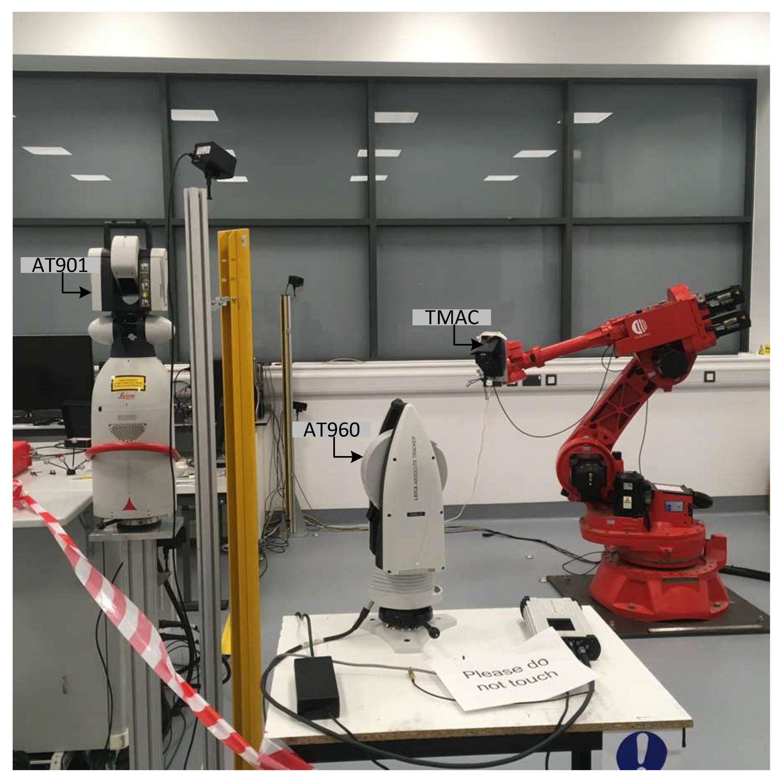
To conduct the verifications, a physical setup was arranged within the cell, as illustrated in Figure 14. In this setup, the NRTEC system, equipped with the Leica Tracker AT901, and the test system developed with ART were simultaneously operated. This parallel operation allowed for the collection of data from both systems at the exact same time, enabling a direct and accurate comparison of their performance and correction capabilities.

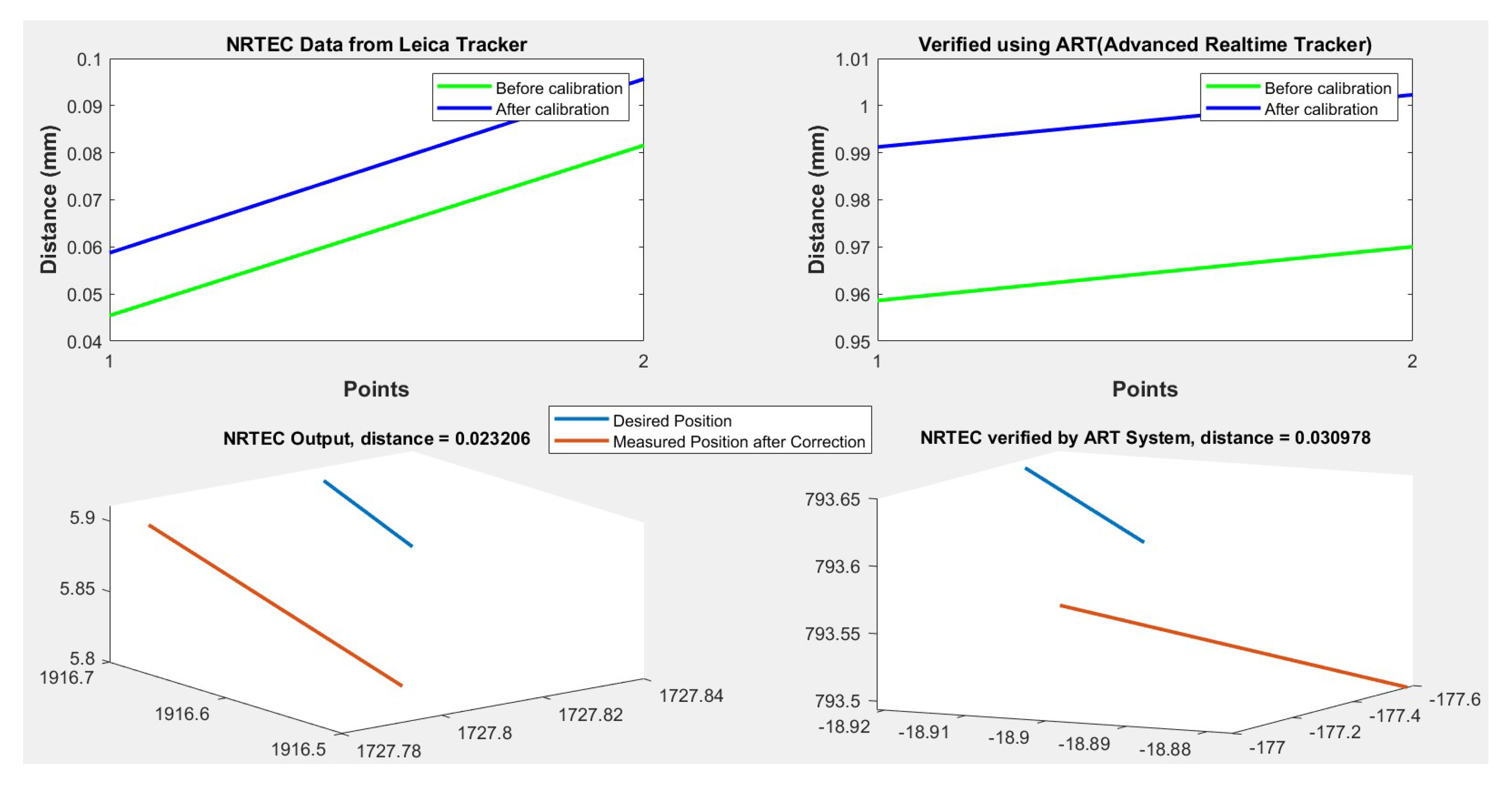
The following is the result. Figure 15 is the plot of two points of corrected and uncorrected data in the Leica Tracker frame and in the ART Coordinate System. The verifications are performed in 6DoF. The graphs on the left side are the data taken by NRTEC. The graphs on the right side display the data taken by using the ART system. The left and right side has two graphs each. The top one shows the 3D points in the space of 2D. The bottom ones show the original 3D points in an X, Y, Z axis. The points are different for both NRTEC and ART systems, as the systems are physically on different locations and give different value for the same point because of that reason. The physical distance can be observed in Figure 15. The distance between two lines is displayed on the bottom graphs. The blue lines on the graph show the desired position which is planned for the robot path, and the red lines on the graph show the data collected after performing the calibration process. The distance between the desired and measured points’ data is displayed on the bottom 3D graphs.

The results obtained from the analysis of the bottom 3D graphs indicate that there is a difference between the desired position and the measured position after the calibration process. For the NRTEC system (graph on the bottom-left), the distance between these two lines is calculated to be 0.023206, while for the ART system (graph on the bottom-right), the distance is measured to be 0.0030978.

Based on these results, the NRTEC system claims to have achieved a correction of approximately 0.02 mm, whereas the ART system verifies the correction to be around 0.03 mm. Therefore, the ART system’s verification supports the claim that the NRTEC system has achieved an accuracy level of up to 0.03 mm.

3.5. System Verification Using AT960

The AT960 Leica Tracker system was utilised to verify the corrections made by the NRTEC system. The AT960 system offers an accuracy of +/−15 µm when used in conjunction with the TMAC, and it has a high measurement capacity of 210,000 points per second.

To obtain the 3D points, the AT960 Leica Tracker was used in the experimental setup. The physical configuration of the cell where the testing took place is illustrated in Figure 16. Both the NRTEC system with AT901 and the test system developed with AT960 were simultaneously operated to ensure the collection of data for accurate comparison.

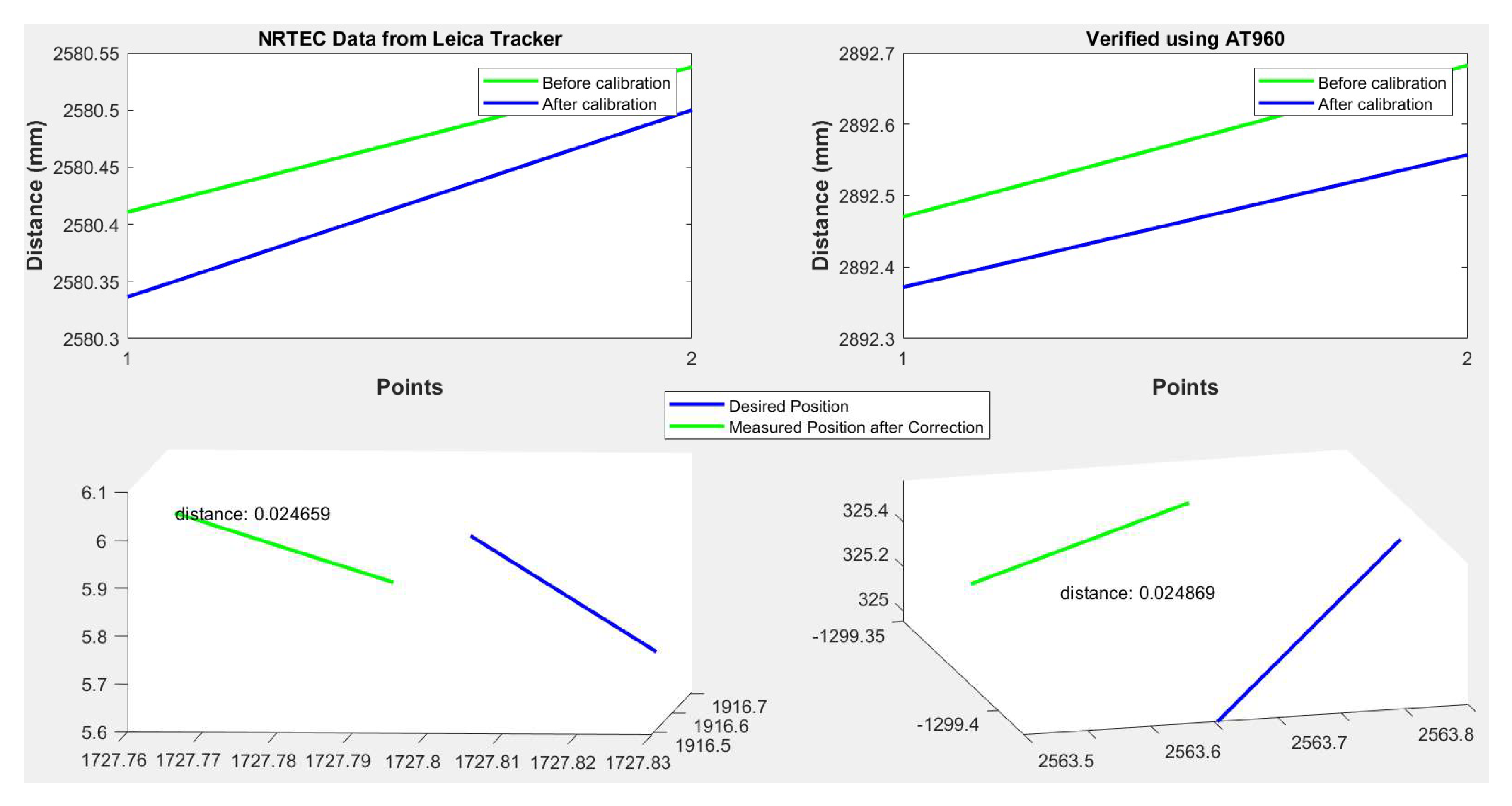
A system was developed to retrieve the points using the AT960 SDK (Software Development Kit). The obtained results are presented below Figure 17. illustrates the plot of two points, depicting both corrected and uncorrected data in the Leica Tracker frame and the AT960 Coordinate System. The verifications were conducted using three degrees of freedom (3DoF) on the AT960 system.

Due to the physical attachment of the TMAC to the AT901 using a wire, it acts as a 3D reflector for the AT960 system. Therefore, the data cannot be collected in six degrees of freedom (6DoF) format from the AT960. The left side of the graphs represents the data collected using the Leica Tracker AT901, while the right side displays the data collected using the AT960 system. Each side consists of two graphs: the top graph shows the 3D points in a 2D space, while the bottom graph illustrates the original 3D points in the X, Y, and Z axes.

The points obtained by both the NRTEC and AT960 systems differ since the trackers are physically located in different positions, resulting in varying values for the same point. The physical distance between the two systems can be observed in Figure 17. The distance between the lines depicted in the bottom graphs indicates the difference between the corrected and uncorrected data. The green lines represent the data collected prior to initiating the calibration process, while the blue lines represent the data collected after performing the calibration process. The discrepancy between the corrected and uncorrected data is displayed in the bottom 3D graphs.

The distance between the desired positions and measured positions for NRTEC is 0.024659, while the distance between those lines using the AT960 system is 0.024869. This indicates that the AT960 system aligns with the correction measurements of NRTEC, validating its accuracy.

The graph below in Figure 18 represents the difference between corrected and uncorrected points using both trackers. It illustrates the error correction captured by both the AT960 and NRTEC trackers. The graph displays 6 points in the X, Y, and Z axes in both positive and negative directions. The difference between the corrected and uncorrected points, as measured by the AT960 and NRTEC systems, is indicated by the red error bars.

The error bars have been drawn to depict the delta range between ±0.000015 and ±0.001029. The error bars are very small, indicating that the difference in the correction measurements performed by both systems is negligible. The data displayed by the error bars demonstrate the reliability of the NRTEC system in comparison to the AT960 system.

Based on the verifications and comparisons with independent systems such as K-Robot, ARTTRACK, and AT960, it has been confirmed that the NRTEC system achieves an accuracy of up to 0.02 mm. The results obtained from these independent systems align with the claimed error correction capabilities of NRTEC, further validating its accuracy and performance.

3.6. Verification Results

The NRTEC system has undergone verification by three independent systems: AT960 Laser Tracker, ART, and K-Robot Camera. Figure 19 showcases the verification of error correction performed by these systems on the NRTEC system. The ART and K-Robot systems validate the correction achieved by NRTEC to be around 0.03 mm. However, the AT960 system, which closely resembles NRTEC’s measurement device AT901, confirms the correction claimed by NRTEC to be around 0.02 mm.

It should be noted that there are certain limitations associated with K-Robot, as it was used in a camera capacity, and only 3D data could be retrieved from the screen. On the other hand, the ART system utilises four cameras and provides data in 6D. The ART system verifies NRTEC’s claim up to 0.030978 mm. While the ART system’s accuracy in 2D is reported to be 0.04 pixels, which is equivalent to 0.0105 mm (10 µm) according to UnitConverters.net (2008), there is no available reference or technical information regarding its accuracy in 3D or 6D. In contrast, the AT960 system has an accuracy of 15 µm in 3D according to Metrology (2015).

Based on the available accuracy information for the ART and AT960 systems, it can be concluded that NRTEC is capable of achieving the claimed accuracy of around 0.02 mm.

4. Discussion and Conclusions

The interactions between the robot’s position, orientation, control inputs, and measurements involve non-linear relationships due to the complex nature of robotic motion and sensor readings. The incorporation of the DRM further adds to the non-linearity as it involves predicting positions and compensating for errors in a dynamic environment. As a result, the overall system is best described as non-linear due to the complex interactions and relationships between various variables and components.

Testing conducted with 100% network load demonstrated that the system operated without delays. Dead Reckoning addresses network latency by replicating the environment on the other side/node of the network, effectively hiding the latency issue. The system aims to achieve realtime error correction by utilizing a network-based control system, enabling continuous correction without the need for a measure, stop, and correct approach. A Neural Network and Kalman Filter are utilised to improve the correction process, while the Realtime Control System (NI CRIO) provides a suitable platform for network control. Additionally, the cost-effectiveness of the metrology device is achieved by utilizing the Flexa system, allowing multiple machines or robots to use the device through network setup. The implementation of DRM compensates for potential disruptions caused by network traffic, ensuring accurate error correction by predicting and compensating for inaccuracies.

Figure 20 illustrates the data collected at different robot positions during the testing process. Each set of robot positions includes variations in the X, Y, Z axes, as well as rotations in the RX, RY, and RZ axes. The data reveals that after a certain number of correction cycles, the rate of error reduction reaches a plateau. Specific data points have been highlighted to evaluate the differences.

In the first graph (top-left), it can be observed that at cycle 15, the achieved error reduction was 0.0254 mm. Comparatively, at cycle 29, the error reduction was 0.02535 mm, indicating a very minor difference of 0.00005 mm. Continuing the correction cycles beyond cycle 15 only impacts the error reduction in nanometres. Similarly, in the fourth graph (middle-right), where 34 cycles of correction were performed, the difference in error reduction between cycle 17 and cycle 30 is only 10 nanometres. The remaining four data sets exhibit a similar trend. The optimal number of cycles depends on the nature of the application and its accuracy requirements. For this particular study, the cycles were stopped at the point where the improvement in error reduction was in the micrometre range. Based on the graphs below, the optimal number of cycles was determined to be between 15 and 17.

The system achieves the correction threshold of 0.02 mm after 15 cycles, with no further improvement observed. Each cycle takes 225 min, and the overall experimentation and data compilation require approximately 6 weeks. The system demonstrates its learning capability as the accuracy improves with repeated robot path execution. This enhancement is achieved through Neural Network based MPC, enabling the system to learn and correct errors at each path point. After completing the 15 cycles, the Leica Tracker can be disconnected and utilised by other systems as needed.

The system has made significant progress in achieving error correction of 0.02 mm after 15 iterations. This precision has been accomplished by effectively handling network delays through the innovative use of DRM, which leverages gaming technology algorithms. Notably, the system has been rigorously tested and proven to deliver a reliable performance even in busy network environments.

The decision to transition from PID (Proportional-Integral-Derivative) control to MPC was primarily driven by the system’s evolving requirements related to multiple inputs and outputs. During the initial stage of the research, PID control sufficed as it provided a simple and straightforward approach for static positional calculations in the three-dimensional space.

However, as the research progressed, the system encountered the need to operate within a normal open network, specifically the university campus network. This posed challenges due to significant packet delays experienced before and after the application of DRM. To address these issues and enhance the system’s performance and adaptability, the decision was made to introduce the DRM.

By incorporating MPC into the control architecture, the system gained several advantages. Firstly, MPC enabled simultaneous optimisation of control actions for all inputs and outputs, accommodating the system’s multiple requirements more comprehensively. Secondly, MPC’s predictive control capabilities allowed for the proactive handling of time-varying dynamics and consideration of network delays, ensuring optimal control decisions based on the anticipated future behaviour. Moreover, MPC’s ability to handle constraints facilitated the effective management of system limitations and boundaries on parameters such as position and speed.

The utilisation of MPC reflects the system’s commitment to achieving high performance and robustness. It offers the flexibility to integrate advanced algorithms and strategies, enabling adaptation to changing network conditions. Furthermore, the adoption of MPC ensures future adaptability and flexibility, facilitating the incorporation of additional variables, constraints, and objectives as the research progresses.

The adoption of MPC was motivated by the system’s evolving needs, including multiple inputs and outputs, time-varying dynamics, and the management of constraints. The system’s impressive error correction results, coupled with the ability to handle network delays through DRM, highlight the effectiveness and suitability of MPC in enhancing performance and adaptability within this complex environment.

Figure 21 presents the average completion time in seconds for moves within each cycle. The orange line represents data from the system’s stage 1, where PID control was implemented without DRM. The highest average time occurred during the 3rd cycle at stage 1, taking 1498 ms to complete a move. The graph illustrates the performance improvement in terms of time after the implementation of DRM and MPC. Despite some remaining delays, DRM allows for local predicted error calculations using players. The average move time reduced from 1401.467 ms in 15 cycles at stage 1 to an average of 758.8667 ms, which is a 46% decrease after DRM and MPC implementation. The change in robot manipulators between stages 1 and 2 has a minimal impact, since the same equipment is utilised.

Notably, the graph reveals the trend of move completion times as cycles progress within each stage. In stage 1, the average time to complete a point remains consistent across cycles. However, in stage 2, there is a significant reduction from 895 s in the first cycle to 663 s, indicating the system’s learning capability and improved error prediction with repeated path executions.

In summary, the system successfully handles network delays and achieves realtime error correction. Utilising advanced algorithms and techniques, the system improves its performance and accuracy over multiple cycles. The cost-effectiveness of the metrology device is achieved through a flexible setup that allows its use by multiple machines. By predicting and compensating for inaccuracies, the system ensures accurate error correction even in the presence of network traffic disruptions. The analysis of data collected at different robot positions reveals that the optimal number of correction cycles falls between 15 and 17. The system demonstrates its learning capability, as accuracy improves with repeated execution of the robot’s path. The transition from a previous control approach to the current system was driven by the evolving requirements and challenges posed by the network environment. The system’s current approach offers improved optimisation, control prediction, and constraint handling, resulting in high performance and adaptability. The system’s adoption of these techniques highlights its commitment to achieving accurate and reliable performance, even in challenging network conditions.