Article

An Adaptive Torque Observer Based on Fuzzy Inference for Flexible Joint Application

1
School of Mechanical Science and Engineering, Huazhong University of Science and Technology, Wuhan 430074, China
2
School of Electrical Engineering and Automation, Wuhan University, Wuhan 430074, China
3
Wuhan Jiutong Intelligent Technology Co., Ltd., Wuhan 430074, China
*
Author to whom correspondence should be addressed.
Machines 2023, 11(8), 794; https://doi.org/10.3390/machines11080794
Submission received: 27 June 2023 / Revised: 28 July 2023 / Accepted: 1 August 2023 / Published: 1 August 2023

Abstract

:
Torque observation techniques have been widely employed to estimate the load torque of flexible joints driven by a permanent magnet synchronous machine (PMSM). However, the performance of the observer degrades significantly when the position and orientation of the robot continuously changes, resulting in substantial irregular load variations. In this paper, an adaptive torque observer based on fuzzy inference is proposed to overcome this issue. Instead of relying on theoretical or numerical derivation, the relationship between the load inertia and the closed-loop poles of the torque observer is expressed by fuzzy inference. This approach enables the flexible configuration of the poles based on the load inertia, allowing for automatic tuning of the gain matrix. Consequently, the observer can ensure robustness and maintain superior performance under varying load conditions. The effectiveness of the proposed observer is validated through simulation and experimental results. It shows that compared to the classical Luenberger observer, the proposed adaptive torque observer can achieve more accurate observation results and exhibits a more dynamic response in the presence of varying load inertia.

1. Introduction

Collaborative robots driven by a permanent magnet synchronous machine (PMSM) are now widely used in various applications, particularly in industrial automation. To achieve superior external force control and motion control performance while ensuring the safety of human–robot collaboration, the utilization of joint torque feedback (JTF) technology is crucial and has gained significant recognition in the robotics community [1,2,3]. Real-time measurement or estimation of the joint load torque is necessary in order to achieve precise JTF control performance.
Currently, torque sensors based on strain gauges [4], optical sensors [5], or encoders [6] are commonly employed to measure joint torque. However, the use of torque sensors unavoidably increases the size, weight, and cost of the joints, while also reducing their reliability and maintainability. Furthermore, the inclusion of torque sensors introduces an additional elastic chain that affects the accuracy of joint control.
To tackle this issue, the industry has shifted its research focus towards torque observation techniques, which have emerged as an important research direction due to their efficiency, cost-effectiveness, and convenience in obtaining the joint load torque with minimal mechanical modifications. Several torque observation techniques have been proposed to estimate the load torque of flexible joints, such as a disturbance observer [7], sliding mode observer [8], Kalman filter [9], and Luenberger observer [10].
Due to its simplicity in parameter selection and flexibility in implementation, the Luenberger observer is widely used in industrial applications. However, it lacks sufficient robustness against measurement noise and parameter mismatch. Achieving proper performance requires a suitable selection of the observer gain matrix, which becomes challenging under various load conditions. Researchers have conducted exploratory research to address these issues. In [11], the left-shifting pole-placement method, which is widely used, is implemented. The observer gain matrix is considered as a general function to satisfy multiple conditions. However, it lacks analysis and comparison of the observer performance in the full-speed region. In [12], the gain matrix is derived at a specific rotational speed and scaled linearly with the speed as it varies. But this approach may cause instability due to the high imaginary part of observer poles. Thus, the root locus for the entire speed range is used to optimize the pole assignment, considering the trade-off between response time and robustness. In [13], an adaptive law is deduced based on adaptive control theory by correcting the error between the adjustable model and the reference model. Consequently, the gain matrix of the observer can be calculated accordingly. In [14], the observer gain matrix is calculated through a series of numerical equations derived by adopting a proportional and integral adaptive scheme. Additionally, some scholars have employed optimization algorithms to design the Luenberger observer gain matrix, for instance, the grey wolf optimizer algorithm [15], the numerically nonlinear least squares algorithm [16], and the H optimization algorithm [17].
The fuzzy system is recognized for its ability to express complex relationships that are not easily captured by classical logic. It is particularly suitable for situations involving significant uncertainties or unknown variations in plant parameters and structures [18,19,20,21]. In this paper, the relationship between the load and the closed-loop poles of the torque observer is expressed by using fuzzy inference, rather than relying on theoretical or numerical derivation. Thus, an adaptive load torque observer is proposed and implemented, demonstrating its capability to ensure robustness and maintain superior performance across various load conditions.
The paper is organized as follows. In Section 2, the dynamic model of the flexible joint is presented. Then, in Section 3, the shortcoming of the classical Luenberger torque observer under load variations are presented. In Section 4, to address the shortcoming, an adaptive torque observer—which is based on the classical Luenberger observer structure, combining the fuzzy inferencer and online inertia identification technique—is proposed and theoretically explained. Finally, the proposed observer is validated through simulations and experiments, consistently demonstrating superior performance under wide load variations, as shown in Section 5.

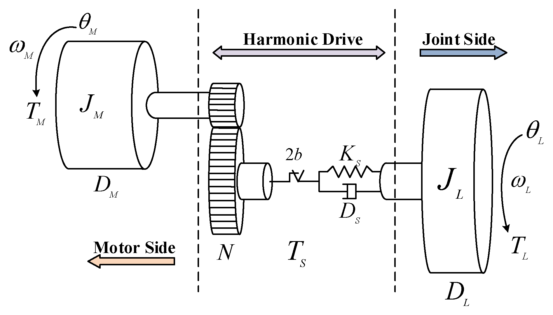
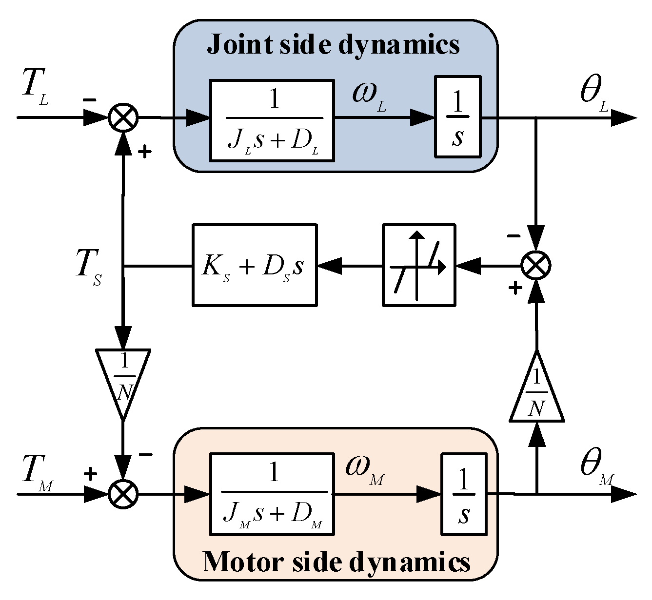
2. System Modeling of Flexible Joint

Figure 1 exhibits a typical transmission model of the flexible joint driven by a PMSM for the use of the cooperative robot, which is mainly composed of a servo motor, a controller, a harmonic drive, a brake, and two encoders. In this model, the harmonic drive is equivalent to the damper-spring system with the stiffness Ks, the damping Ds, the transmission ratio N, and the backlash b. The electromagnetic torque TM and the shaft torque Ts act together on the motor, whose moment of inertia is JM and friction torque coefficient is DM, to decide the motor speed ωM. Meanwhile, the load torque TL and the shaft torque Ts act together on the joint, whose moment of inertia is JL and friction torque coefficient is DL, to decide the load speed ωL.
The system dynamic model of the flexible joint is depicted in Figure 2. Since the collaborative robot joints utilize a harmonic drive with a relatively large transmission ratio to maximize torque density, the transmission backlash can be neglected. As a result, the mathematical model of the system can be derived as Equations (1)–(5):
J M ω ˙ M = T M D M ω M 1 N T S
J L ω ˙ L = T S D L ω L T L
T S = K S ( θ M N θ L ) + D S ( θ ˙ M N θ ˙ L )
ω M = θ ˙ M
ω L = θ ˙ L
It is assumed that the load torque TL = 0 Nm, the transfer function between motor speed ωM, and motor electromagnetic torque TM can be derived as Equation (6):
ω M T M = N 2 ( J L s 2 + D L s + D S s + K S ) ( J L s + D L ) ( K S + D S s ) + ( J M s + D M ) ( ( J L s + D L ) s + D S s + K S )
Assuming that the system damping DM, DS, and DL is neglected, the eigenvalues λp that determine the behavior of the joint model shown in Equation (6) are provided by:
λ p 1 , 2 = 0
λ p 3 , 4 = ± j ( J M + 1 N 2 J L ) K s J M J L

3. Classical Luenberger Torque Observer

3.1. Observer Design

Based on the system dynamic model described in Equations (1)–(5), the state space equations of the flexible joint can be written as:
x ˙ = A x + B u y = C x
where x is the state vector, A is the state matrix, B is the control matrix, C is the output matrix, u is the input signal matrix, and y is the output signal matrix.
The full-order Luenberger observer for state variables x can be defined by the state equations shown below:
x ^ ˙ = A x ^ + B u + L ( y y ^ ) = ( A L C ) x ^ + B u + L y
where x ^ ˙ = [ ω ^ ˙ M ω ^ ˙ L T ^ ˙ J T ^ ˙ L ] T , u = T M , and y = ω M . The state matrix A, control matrix B, output matrix C, and gain matrix L of the Luenberger observer are provided as follows:
A = D M J M 0 1 N J M 0 0 D L J L 1 J L 1 J L K N K 0 0 0 0 0 0 , B = 1 J M 0 0 0 , C = [ 1 0 0 0 ] , L = [ l 1 l 2 l 3 l 4 ] T
The symbol ^ denotes the estimated value of the state variable, and L is the observer gain matrix designed to achieve the required performance of the observer. Since both the matrixes [B AB A2B A3B] and [C CA CA2 CA3] are full rank, the plant system is controllable and observable.
The estimation error of state variables is e = x x ^ . To ensure that the observation error of the state variables converges to zero, the observer gain matrix needs to be reasonably designed. As we know, the pole placement method is a well-established method for gain matrix design. According to this method, the closed-loop poles λP of the observer should be configured in the negative half-axis region, that is Re(A-LC)] < 0, to make the state matrix (A-LC) of the observer asymptotic stable. Thus, the observer gain matrix L can be solved according to Equation (12). To reduce matrix operation and improve the DSP calculation efficiency of the servo driver, the poles of the observer are usually configured at the same point on the negative half-axis. As a result, it can be obtained that:
f ( s ) = s I ( A L C ) = ( s λ ) 4
According to Equation (12), the gain matrix L can be computed as follows:
l 1 = 4 λ D M J M D L J L
l 2 = N J M ( D L 3 + 4 λ D L 2 J L + 6 λ 2 D L J L 2 + 4 λ 3 J L 3 2 D L J L K S 4 λ J L 2 K S ) J L 3 K S
l 3 = N 2 D L 2 J M + 4 N 2 λ D L J L J M + 6 N 2 λ 2 J L 2 J M J L 2 K S N 2 J L J M K S N J L 2
l 4 = N λ 4 J M J L K S
The aforementioned equations enable the closed-loop poles of the observer to be placed in desired positions. However, it is important to consider the distance between the pole configuration and the origin of the observer. If the distance is less than that of the plants, the observer will be unable to accurately capture the real-time response of the system state. On the other hand, if the observer pole configuration is too large, it will amplify measurement noise, leading to erroneous observation results. Therefore, it is necessary to allocate the observer poles to account for parameter variations while maintaining performances. Furthermore, it is crucial to note that both measurement noise and parameter mismatches significantly impact the stability and effectiveness of the pole configuration. In other words, the key aspect of designing the torque observer for the flexible joint lies in the reasonable allocation of closed-loop poles considering parameter variations.

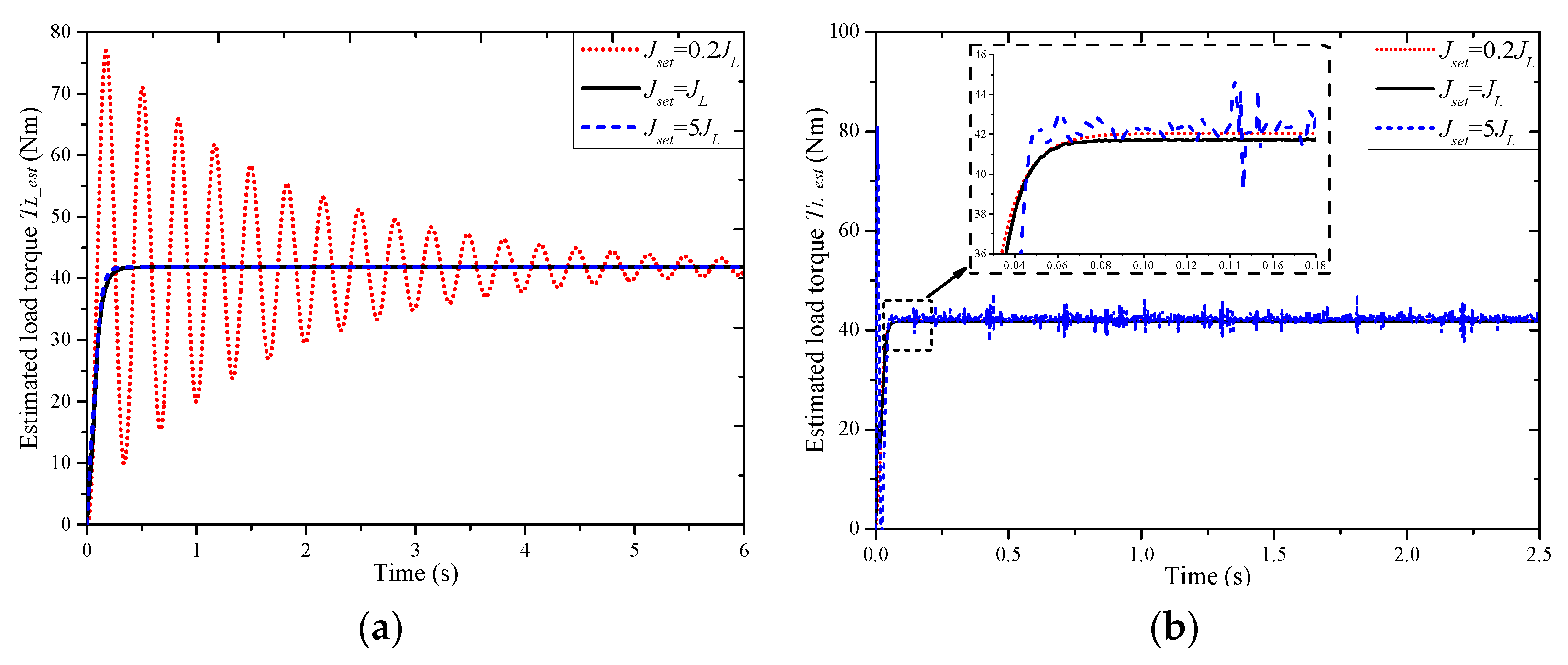
3.2. Observer Performance Analysis

The torque observer utilized in the flexible joint demonstrates reasonable robustness, as discussed in Section 3.1. However, parameter mismatches can lead to an unstable dynamic response. The stiffness Ks of the harmonic drive, the moment of inertia JM, and the friction torque coefficient DM can be accurately obtained from the manufacturer datasheet. Nevertheless, in many applications, the load of the joint varies greatly, which can significantly degrade the performance of the torque observer. If the gain matrix of the observer remains fixed, the performance cannot be guaranteed when the load inertia of the flexible joint is substantially higher than the original inertia. The following provides a quantitative explanation, as derived from Equation (2):
T L = T S D L ω L J L ω ˙ L = T S ( D ^ L + Δ D L ) ω L ( J ^ L + Δ J L ) ω ˙ L
where Δ J L = J L J ^ L is the difference between the nominal and actual load inertias, and Δ D L = D L D ^ L is the difference between the nominal and the actual load friction torque coefficients. It is important to note that when there are differences between the nominal and actual parameters, the estimated load torque will be contaminated by inaccurate system parameters.
An offline parameter identification method is used to calibrate the load friction torque coefficients. The result of the calibration test is provided in Figure 3. According to the test result, the viscous friction torque coefficient of the joint is 5.5 × 10⁻⁴ Nm·s/rad and the Coulomb torque friction coefficient is 0.0435 Nm. The speed and friction torque correspondence table can be used to compensate for torque observation error caused by the mismatch of friction coefficients.
It should be noted that during the operation of the cooperative robot, the position and orientation of the robot arm continuously changes. Thus, the equivalent load inertia and load torque of each joint also undergo constant variations. Therefore, the offline parameter identification method is not suitable in this scenario.
Subsequently, simulation and experimental results are used to estimate the influence of load inertia mismatch on observer performance. The specification of the flexible joint is presented in Table 1. In the simulation, a constant load is applied to the flexible joint at time t = 0 s, with the load torque TL = 43 Nm and the load inertia JL = 2 kg·m2. Band-limited white noises are introduced to the measurement signal of motor speed ωM and motor current IM, simulating the measurement noise from encoders and current sensors.
When the closed-loop poles of the torque observer are configured at λP = −50, the load torque can be accurately estimated within 0.4 s if there is no parameters mismatch of load inertia JL, as depicted by the solid line in Figure 4a. The dotted line and dashed line in Figure 4a represent the simulation results when the load inertia is changed to 0.2 times and 5 times, respectively. It can be seen that when there is a load inertia mismatch (Jset = 0.2 JL), the observer torque exhibits a larger overshoot and takes longer to reach a steady state. Conversely, if the load inertia of the torque observer is set to a value greater than the actual inertia (Jset = 5 JL), the observer torque curve remains similar, although the estimated torque error is larger.
While the poles of the observer are set at λP = −200, as illustrated in Figure 4b, the load torque is accurately estimated within 0.1 s, which is significantly faster than the poles are configured at λP = −50. This is because placing the poles farther results in a larger gain matrix for the observer, leading to a faster response. However, it should be noted that when the load inertia of the torque observer is set to a value greater than the actual inertia (Jset = 5 JL), a considerably higher estimated torque error occurs, primarily due to measurement noise.
To verify the simulation results in Figure 4, experimental results are presented under the same load inertia variations in Figure 5. In the experiment, the sampling periods for the position-loop and speed-loop are 200 μs, while the sampling period of the current-loop is 100 μs. The joint is operated in position control mode to keep the load test tooling in a horizontal position while a 7.5 kg mass disc is mounted on it, of which the load torque TL = 43.6 Nm and the load inertia JL = 2.15 kg·m2. When the poles of the observer are configured at λP = −50, it can be observed from Figure 5a that the estimated load torque requires over 6 s oscillations to stabilize when Jset = 0.2 JL. This is due to the relatively small observer gain in this pole configuration, resulting in a long stabilization time. However, for Jset = JL and Jset = 5 JL, the observer gain is appropriate without amplifying the measurement noise. On the other hand, when the observer poles are set at λP = −200, as shown in Figure 5b, the estimated load torque stabilizes within approximately 0.1 s, which is much faster compared to the configuration with λP = −50 when Jset = 0.2 JL and Jset = JL. However, when Jset = 5 JL, the large observer gain leads to an overshoot of nearly 100% and significantly amplifies the measurement noise.
The simulation and experimental results demonstrate that the classical Luenberger torque observer, with a fixed gain matrix L, exhibits deteriorated performance when there are significant variations in the load inertia. Consequently, to achieve more accurate load torque observation results, it is necessary to identify the load inertia and employ an adaptive pole placement strategy. By adopting the observer poles configuration based on the varying load inertia, it becomes possible to enhance the performance and obtain more precise estimations of the load torque.

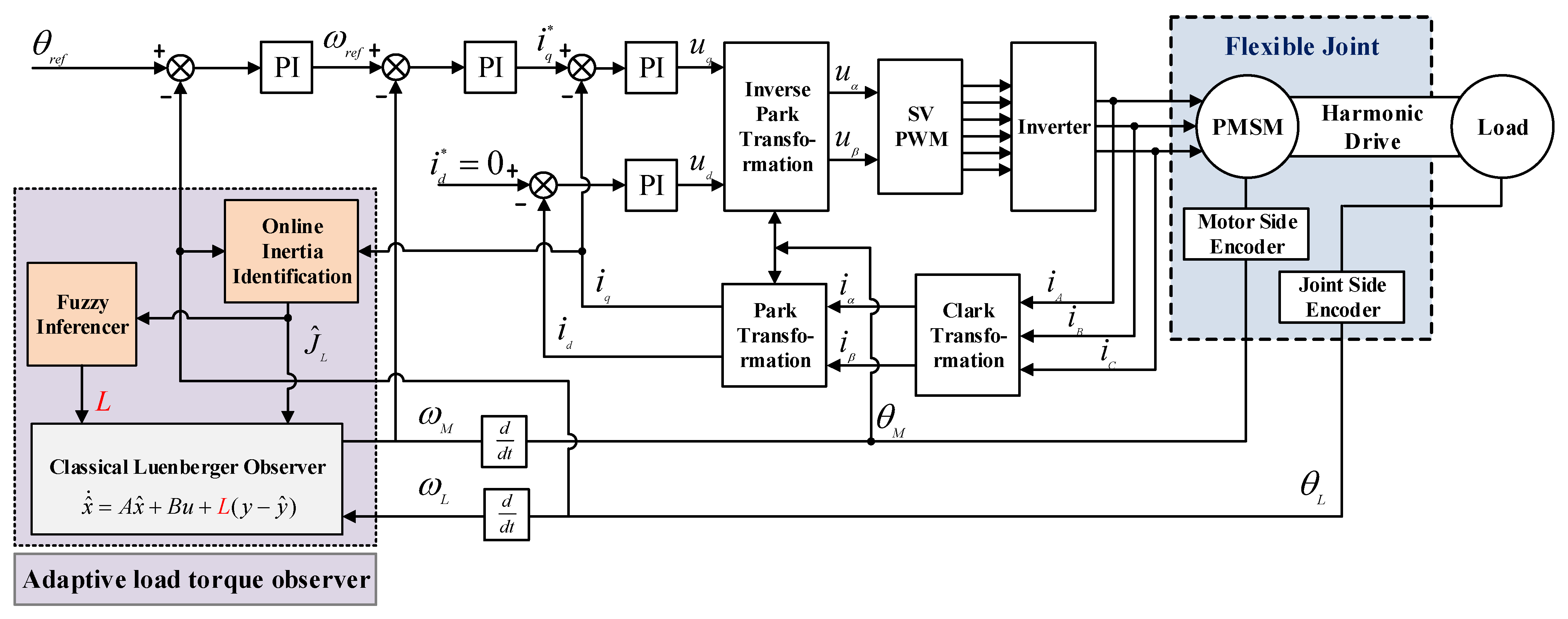
4. Fuzzy Inference-Based Torque Observer

As discussed in Section 3.2, the pole placement method is utilized for designing the gain matrix of the torque observer. Based on control theory, the poles of the observer are typically selected to converge 10 times faster than those of the plant system, striking a tradeoff between responsiveness and stability [22]. In this section, an adaptive load torque observer is proposed, as shown in Figure 6. The main difference between the proposed torque observer and the classical Luenberger torque observer is that the gain matrix L can be autotuned online as the load varies. For the classical Luenberger torque observer, the gain matrix L is derived theoretically or numerically at rated condition. For the proposed observer, the relationship between the load and the gain matrix L is expressed by using the fuzzy inferencer with online inertia identification. This approach enables the establishment of a practical performance relationship between the closed-loop poles λP and the load inertia JL. By leveraging expert knowledge derived from simulation and experimental results, the adaptive observer can ensure superior performance across various load conditions. The fuzzy inference method is chosen for its effective handling of nonlinear control tasks and suitability for modeling and controlling complex, ill-defined dynamic processes [23,24].

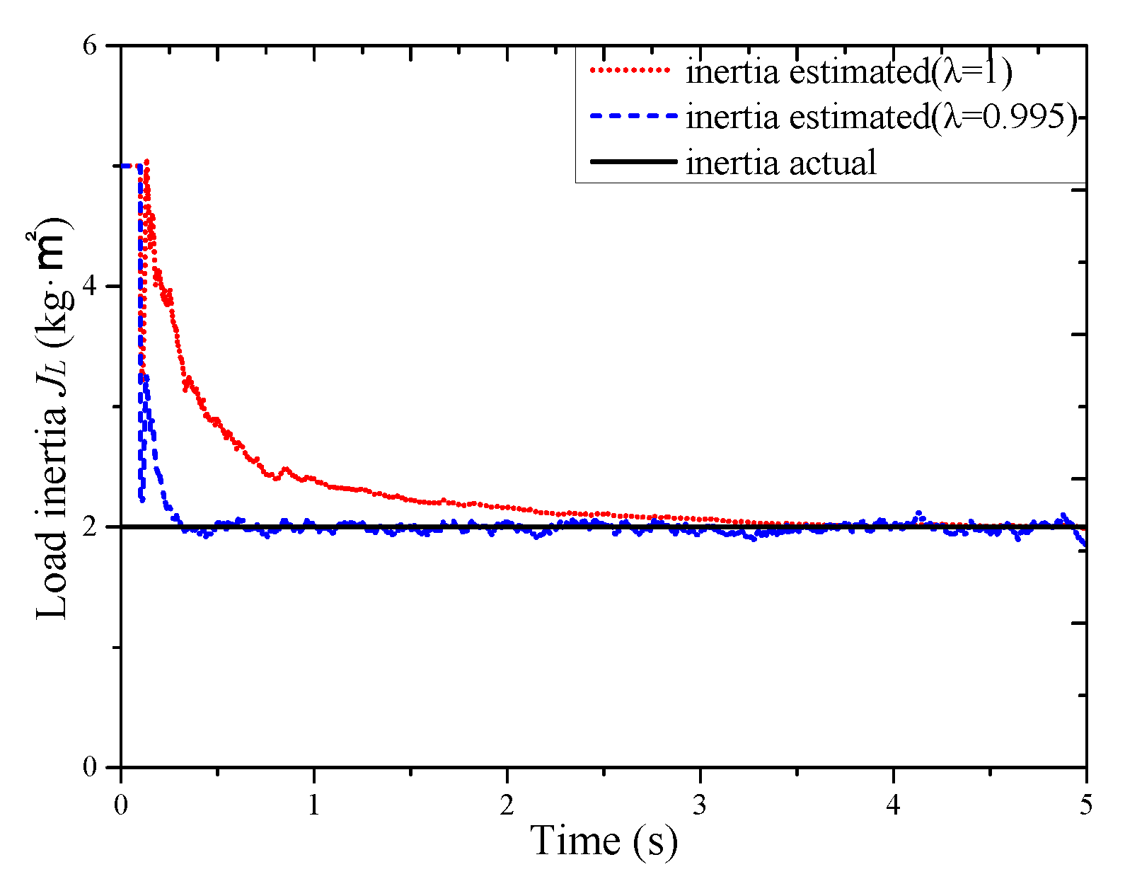
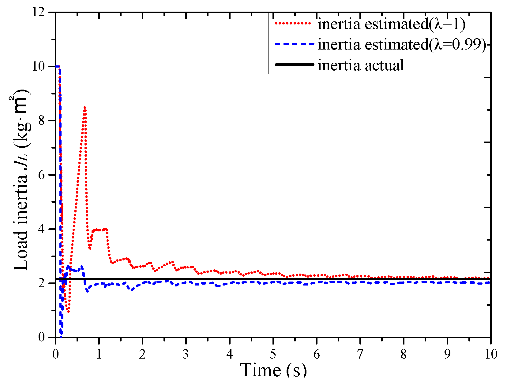
4.1. Online Inertia Identification

To mitigate the impact of load inertia mismatch, an online parameter identification method is necessary. In [25], an inertia identification method based on the speed response is presented which employs sinusoidal rotational speed as excitation. In [26], the researchers utilize a disturbance observer to estimate external disturbances and friction in the model, subsequently obtaining an estimate of inertia. Comparatively, the sliding mode observer offers advantages such as robustness against disturbances and low sensitivity to parameter variations throughout the system [27]. Additionally, the model reference adaptive method [28] and recursive least squares method [29] are viable options for online inertia identification in servo systems.
In this paper, the forgetting factor recursive least squares (FFRLS) method, which is straightforward to implement and avoids data saturation in the recursion process, is adopted to identify the load inertia. Given the sufficiently high sampling frequency of the servo driver, the inertia identification expression for the flexible joint, based on FFRLS, can be derived as follows:
ω M ( n ) = ( 1 D t s J ) ω M ( n 1 ) + t s J T M ( n 1 ) t s J T L ( n 1 )
where ts is the sampling time. According to the FFRLS method design rules, Equations (19)–(23) can be obtained:
θ ( n ) = θ ( n 1 ) + K ( n ) [ y ( n ) φ T ( n ) θ ( n 1 ) ]
P ( n ) = 1 λ [ I K ( n ) φ T ( n ) ] P ( n 1 )
K ( n ) = P ( n 1 ) φ ( n ) λ + φ T ( n ) P ( n 1 ) φ ( n )
θ ( n 1 ) = [ 1 D t s J , t s J , t s J T L ( n 2 ) ] T
φ ( n ) = [ ω M ( n 1 ) , T M ( n 1 ) , 1 ] T
where θ(n) is the estimated value of the parameters at n time, y(n) is the measured motor speed, φ(n) is the input matrix, P(n) is the covariance matrix, K(n) is the gain vector, and λ is the forgetting factor.
The tracking ability and parameter fluctuation of FFRLS are greater with a smaller forgetting factor λ, while they decrease with a larger forgetting factor λ. It should be noted that the identified inertia, as stated in Equation (18), represents the total inertia of the flexible joint with the load. Once the motor inertia JM is obtained from the manufacturer datasheet, the load inertia JL can be calculated accordingly.
J e s t = t s θ ^ K ( 2 ) = J M + 1 N 2 J L

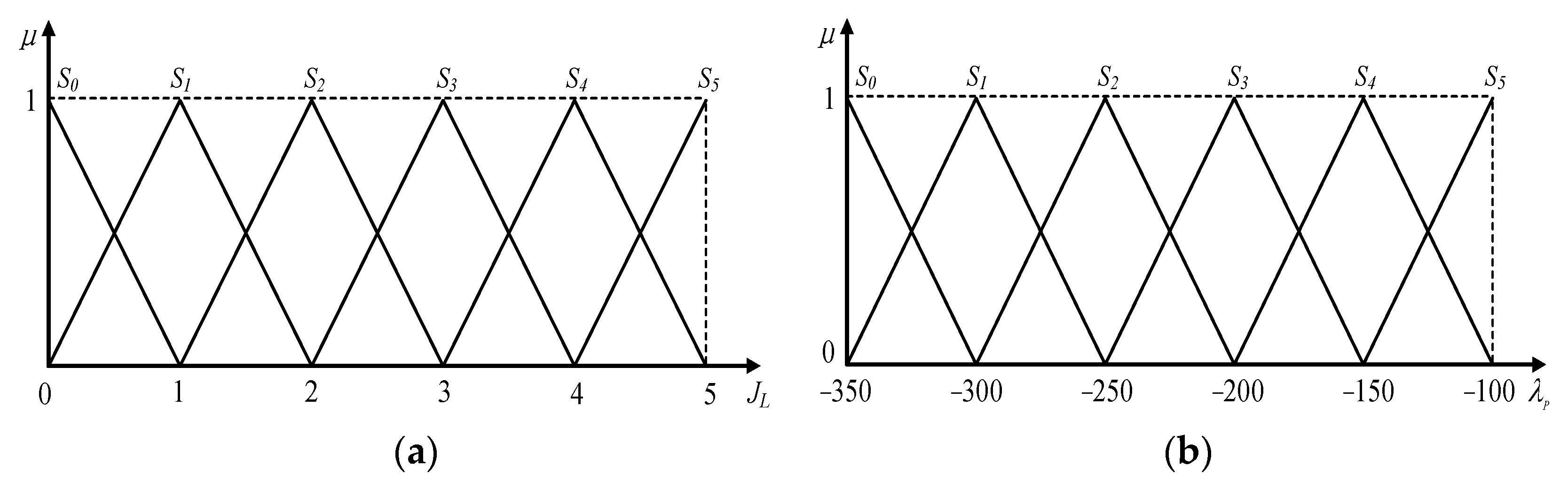
4.2. Adaptive Gain Matrix Design with Fuzzy Inference

A fuzzy inferencer is designed to describe the autotuning function for the configured poles. The fuzzy inferencer follows a Mamdani type, which has one input and one output. With the online inertia identification technique, the load inertia JL is achieved and used as the input of the fuzzy inferencer. The pole λP is utilized as the output of the fuzzy inferencer.
By conducting simulation and experimental tests, the appropriate groups of membership functions and fuzzy rules are determined. Considering the load limit of the designed flexible joint, the range of JL satisfies JL < 5 kg·m2, and the corresponding fuzzy sets are denoted as S0, S1, S2, S3, S4, and S5. The fuzzy set of λP can be chosen as S0, S1, S2, S3, S4, and S5, in which the range is −350 < λP < −100. The membership functions for the input and output variables are represented by triangular membership functions. The locations of the fuzzy membership functions for both input and output, which are evaluated by testing and expert knowledge, are depicted in Figure 7.
The fuzzy inference rules are as follows. If JL is Si, then λP is Si (where i = 0, 1, 2, 3, 4, 5). For each input value, the rule base assigns the corresponding state, and the precise output value is calculated using the defuzzification process. The centroid method, a commonly used approach, is employed as the defuzzification strategy, ensuring both sensitivity and simplicity. The output value λP is calculated as follows:
λ P = i μ ( λ P _ i ) λ P _ i i μ ( λ P _ i )
where μ(λP_i) is the membership value for the point λP_i in the universe of discourse.

5. Simulation and Experimental Results

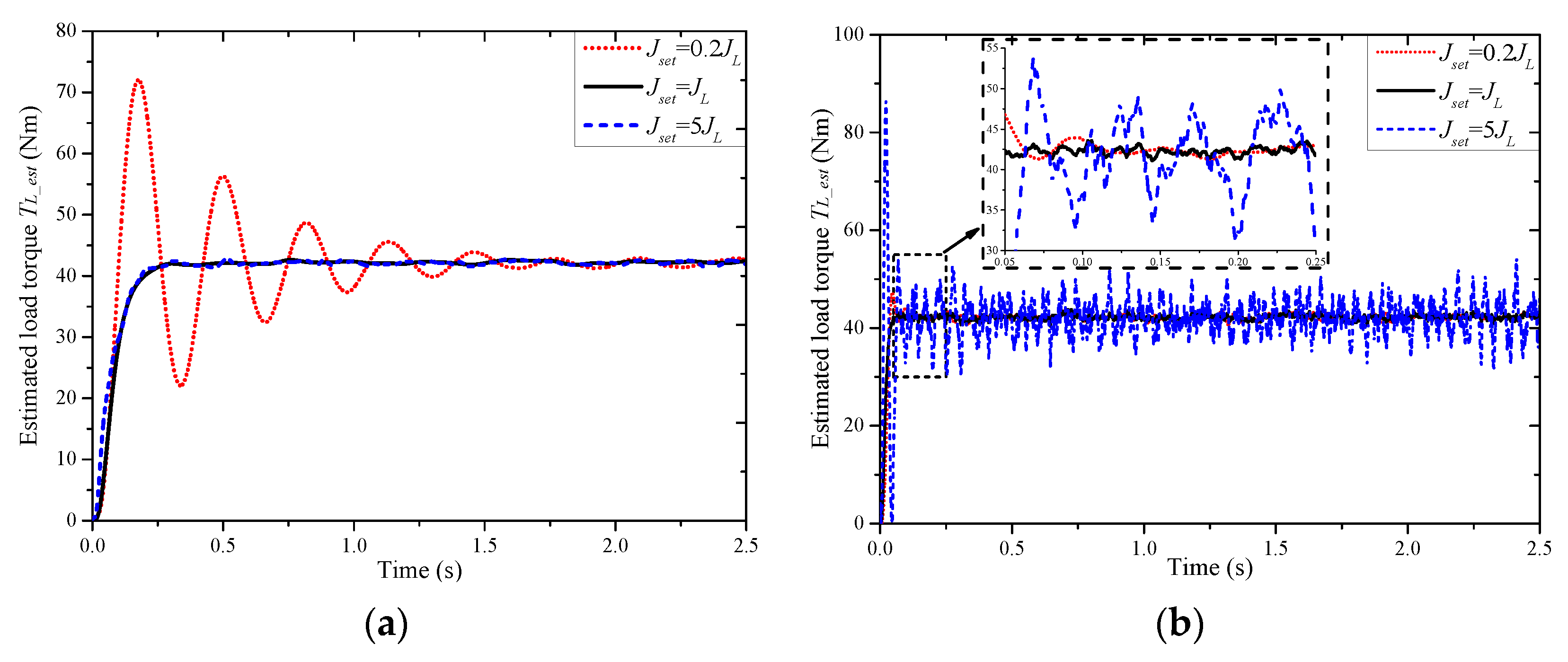
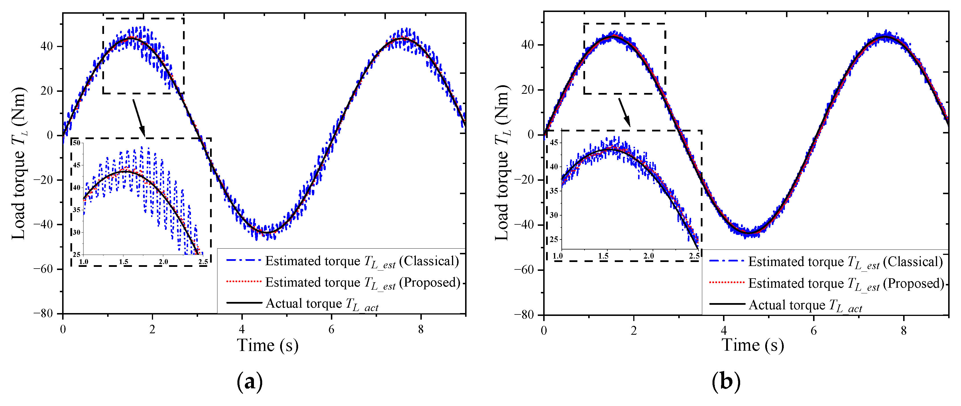
5.1. Simulation Results

The specifications of the flexible joint are presented in Table 1. During the simulation, the joint is operated under constant speed conditions (ωL = 9.9 rpm), and the load torque is set as TL* = 43.6 × sin(πt/3) Nm at t = 0.5 s. The other simulation parameters remain consistent with those described in Section 3.2. The simulation result of online identification of load equivalent inertia based on FFRLS is depicted in Figure 8. It is shown that the inertia identification method (dash line) achieves a satisfactory estimation effect. However, it should be noted that a small forgetting factor λ leads to a rapid identification but compromises the algorithm′s stability.
By employing the fuzzy inferencer designed in Section 4.2, an adaptive pole placement configuration is implemented using online identification of load inertia as input. Initially, the pole location of the observer is set to λP = −250, which yields good observer performance when the load inertia is JL = 2 kg·m2. Subsequently, the load inertia changes to JL = 0.05 kg·m2 while maintaining the same load torque, and the estimated torque comparison between the classical Luenberger torque observer and proposed torque observer when load inertia varies are shown in Figure 9a. It can be found that with the fuzzy inference-based adaptive law, the configured closed-loop poles of the proposed observer λP change from −250 to −329, resulting in the autotuning of the gain matrix. As a result, the proposed torque observer exhibits reduced overshoot and dynamic oscillation due to the variations in load inertia.
Similarly, the results observed when the load inertia changes to JL = 5 kg·m2, in addition to the estimated torque comparison, are presented in Figure 9b. The configured closed-loop poles of the proposed observer λP change from −250 to −116, enabling the autotuning of the gain matrix. The conclusion remains consistent, indicating that the proposed torque observer achieves better performance with the adaptive law. Additionally, it should be noted that the presence of measurement noise leads to a smaller estimated error.

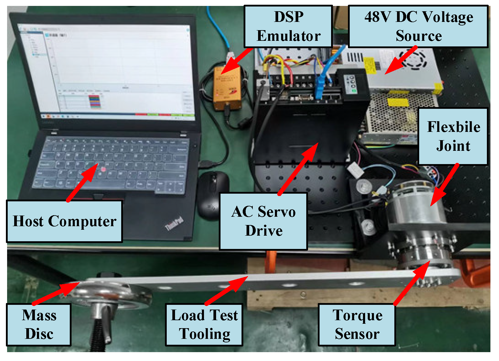
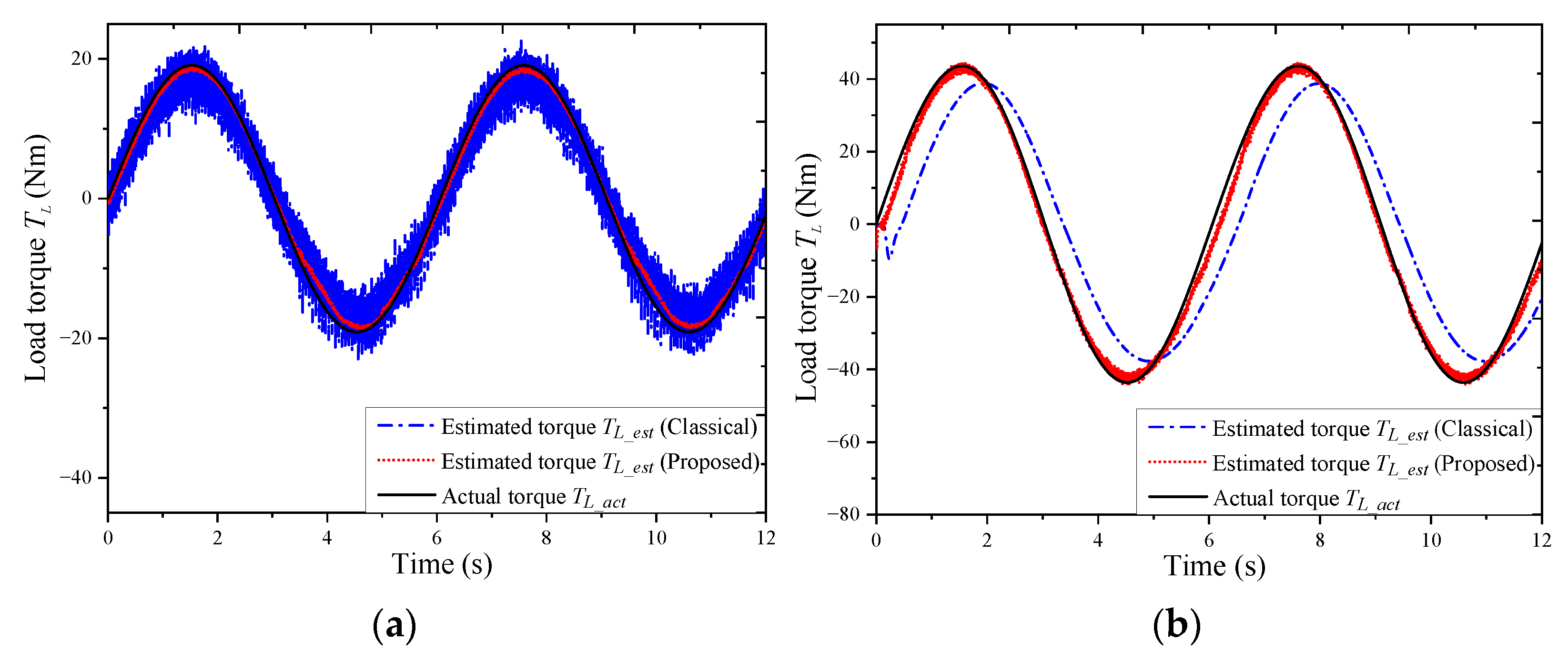
5.2. Experimental Results

To further evaluate the performance of the proposed observer, a test is conducted using the experimental platform depicted in Figure 10. The type of torque sensor is M2210C9. The joint is controlled by a servo drive, in which the DSP STM32F407ZET6 is utilized for implementation with a switching frequency of 10 kHz and a clock frequency of 168 MHz. The sampling periods for the position loop and speed loop are 200 us, and the sampling period of the current loop is 100 us. Two absolute encoders are employed to measure the position of the motor and the joint, with the motor encoder having a resolution of 17 bits and the joint encoder having a resolution of 18 bits. It should be noted that the torque sensor is utilized to obtain the actual value of load torque, which is then compared to the estimated torque.
The joint specification remains the same as stated in Table 1, and other experimental parameters for the test align with those mentioned in Section 3.2. In the test scenario, a load mass disc is attached to the load test tooling through a bolted connection. The load test tooling is constructed from aluminum alloy and has a weight of 1.2 kg, with the distance from the barycenter to the flexible joint measuring 0.24 m. The combined weight of the bolt and nut is 0.9 kg with a distance of 0.5 m from the barycenter to the flexible joint.
Figure 11 illustrates the experimental result of online inertia identification using different forgetting factors when the actual inertia of the system is 2.15 kg·m2. It shows that a small forgetting factor λ yields a real-time response. Although there exists a small error between the identified inertia and the actual inertia, it has minimal impact on the performance of the torque observer. This is because the proposed adaptive observer is less sensitive to variations in load inertia.
Adopting the same test method as described in Section 3.2, the joint is operated in position control mode to maintain the horizontal position of the load test tooling with various mass discs attached to it. The results of the estimated load torque are presented in Table 2, while the actual load torque is directly measured by the torque sensor.
In the experimental conditions, the flexible joint operates in constant speed mode (ωL = 9.9 rpm). At first, a 2.5 kg mass disc is attached, resulting in a load torque TL = 19.1 Nm. With the online inertia identification algorithm, the actual inertia of the load is determined to be JL = 0.9 kg·m2. The experimental performances comparison between a classical Luenberger torque observer and the proposed torque observer when load inertia varies are depicted in Figure 12a. The initial pole location of the classical Luenberger observer is λP = −500, leading to significant measurement noise and estimated torque error. However, with the application of the adaptive law based on fuzzy inference, the configured poles λP are adjusted to −305 of the proposed observer. Consequently, the estimated load torque TL_est = 18.5 Nm with an estimated error of 3.1%. The autotuning of the gain matrix prevents the amplification of measurement noise in the observation results.
Similarly, a test is conducted with a load of 7.5 kg, where the load torque TL = 43.6 Nm and the actual inertia JL = 2.15 kg·m2. The estimated torque comparison is shown in Figure 12b. The initial closed-loop poles location of the classical Luenberger observer is λP = −30, resulting in a significant time delay in the observed torque. However, by employing an adaptive gain matrix L, the configured poles of the proposed observer λP are adjusted to −235. As a result, the estimated load torque TL_est = 42.5 Nm with an estimated error of 2.5%, showcasing a considerable enhancement in the observer performance.
According to the simulation and experimental results, it can be concluded that the proposed adaptive torque observer for flexible joint exhibits superior dynamic performance across various load conditions.

6. Conclusions

The classical Luenberger observer has been proven to yield inaccurate observation results and poor dynamic response when confronted with variations in the load of flexible joints driven by a PMSM. To address this issue, an adaptive torque observer based on fuzzy inference is proposed and implemented in this paper. The approach leverages the FFRLS method for online identification of the load inertia JL, within the framework of the classical Luenberger observer. Subsequently, a fuzzy inference system is utilized to describe the relationship between the load inertia JL and the closed-loop poles λP. This enables the flexible configuration of the gain matrix L of the observer in accordance with the load conditions. Consequently, the observer exhibits superior stability and dynamic performance across a wide range of load variations. Both simulation and experimental results confirm the robustness of the proposed torque observer in achieving more accurate observations and more dynamic responses, particularly in scenarios where the load inertia undergoes significant changes.

Author Contributions

Conceptualization, Y.L. and B.S.; methodology, Y.L. and Y.G.; software, X.Z.; validation, Y.L. and T.C.; formal analysis, Y.L.; investigation, Y.G.; resources, B.S.; data curation, X.Z.; writing—original draft preparation, Y.L.; writing—review and editing, X.Z.; visualization, Y.G.; supervision, B.S.; project administration, T.C.; funding acquisition, B.S. and X.Z. All authors have read and agreed to the published version of the manuscript.

Funding

This research was funded by the Key Research and Development Program of Hubei Province under Grant 2022BAA061 and the Key Research and Development Program of Dongguan City under Grant 20201200300082.

Data Availability Statement

Not applicable.

Conflicts of Interest

The authors declare no conflict of interest.

References

  1. Ruderman, M.; Iwasaki, M. Sensorless torsion control of elastic-joint robots with hysteresis and friction. IEEE Trans. Ind. Electron. 2016, 63, 1889–1899. [Google Scholar] [CrossRef]
  2. Oh, S.; Kong, K. High-precision robust force control of a series elastic actuator. IEEE-ASME Trans. Mechatron. 2017, 22, 71–80. [Google Scholar] [CrossRef]
  3. Zanchettin, A.M.; Ceriani, N.M.; Rocco, P.; Ding, H.; Matthias, B. Safety in human-robot collaborative manufacturing environments: Metrics and control. IEEE Trans. Autom. Sci. Eng. 2016, 13, 882–893. [Google Scholar] [CrossRef] [Green Version]
  4. Albu-Schäffer, A.; Loughlin, C.; Haddadin, S.; Ott, C.; Stemmer, A.; Wimböck, T.; Hirzinger, G. The DLR lightweight robot: Design and control concepts for robots in human environments. Ind. Robot: Int. J. 2007, 34, 376–385. [Google Scholar] [CrossRef] [Green Version]
  5. Hazelden, R. Optical torque sensor for automotive steering systems. Sens. Actuators A: Phys. 1993, 37, 193–197. [Google Scholar] [CrossRef]
  6. Kashiri, N.; Malzahn, J.; Tsagarakis, N.G. On the sensor design of torque controlled actuators: A comparison study of strain gauge and encoder-based principles. IEEE Robot. Autom. Lett. 2017, 2, 1186–1194. [Google Scholar] [CrossRef]
  7. Sariyildiz, E.; Ohnishi, K. Stability and robustness of disturbance-observer-based motion control systems. IEEE Trans. Ind. Electron. 2015, 62, 414–422. [Google Scholar] [CrossRef] [Green Version]
  8. Lu, W.Q.; Zhang, Z.Y.; Wang, D.; Lu, K.Y.; Wu, D.; Ji, K.H.; Guo, L. A new load torque identification sliding mode observer for permanent magnet synchronous machine drive system. IEEE Trans. Power Electron. 2019, 34, 7852–7862. [Google Scholar] [CrossRef]
  9. Shi, Z.G.; Li, Y.K.; Liu, G.J. Adaptive torque estimation of robot joint with harmonic drive transmission. Mech. Syst. Signal Process. 2017, 96, 1–15. [Google Scholar] [CrossRef]
  10. Luenberger, D. An introduction to observers. IEEE Trans. Autom. Control 1971, 16, 596–602. [Google Scholar] [CrossRef]
  11. Ruderman, M.; Ruderman, A.; Bertram, T. Observer-based compensation of additive periodic torque disturbances in permanent magnet motors. IEEE Trans. Ind. Inform. 2013, 9, 1130–1138. [Google Scholar] [CrossRef]
  12. Nguyen, N.D.; Nam, N.N.; Yoon, C.; Lee, Y.I. Speed sensorless model predictive torque control of induction motors using a modified adaptive full-order observer. IEEE Trans. Ind. Electron. 2022, 69, 6162–6172. [Google Scholar] [CrossRef]
  13. Usama, M.; Choi, Y.-O.; Kim, J. Speed sensorless control based on adaptive Luenberger observer for IPMSM drive. In Proceedings of the 19th International Power Electronics and Motion Control Conference, Gliwice, Poland, 25–29 April 2021; pp. 602–607. [Google Scholar]
  14. Kubota, H.; Matsuse, K.; Nakano, T. DSP-based speed adaptive flux observer of induction motor. IEEE Trans. Ind. Appl. 1993, 29, 344–348. [Google Scholar] [CrossRef]
  15. Kaminski, M. Adaptive gradient-based Luenberger observer implemented for electric drive with elastic joint. In Proceedings of the 23rd International Conference on Methods & Models in Automation & Robotics, Miedzyzdroje, Poland, 27–30 August 2018; pp. 53–58. [Google Scholar]
  16. Hu, X.S.; Sun, F.C.; Zou, Y.A. Estimation of state of charge of a Lithium-Ion battery pack for electric vehicles using an adaptive Luenberger observer. Energies 2010, 3, 1586–1603. [Google Scholar] [CrossRef]
  17. Ibaraki, S.; Suryanarayanan, S.; Tomizuka, M. Design of Luenberger state observers using fixed-structure H-infinity optimization and its application to fault detection in lane-keeping control of automated vehicles. IEEE-ASME Trans. Mechatron. 2005, 10, 34–42. [Google Scholar] [CrossRef]
  18. Szabat, K.; Than, T.V.; Kaminski, M. A modified fuzzy Luenberger observer for a two-mass drive system. IEEE Trans. Ind. Inform. 2015, 11, 531–539. [Google Scholar] [CrossRef]
  19. Szabat, K.; Wrobel, K.; Drozdz, K.; Janiszewski, D.; Pajchrowski, T.; Wojcik, A. A fuzzy unscented kalman filter in the adaptive control system of a drive system with a flexible joint. Energies 2020, 13, 2056. [Google Scholar] [CrossRef] [Green Version]
  20. Gholami, A.; Markazi, A.H.D. A new adaptive fuzzy sliding mode observer for a class of MIMO nonlinear systems. Nonlinear Dyn. 2012, 70, 2095–2105. [Google Scholar] [CrossRef]
  21. Li, Z.J.; Su, C.Y.; Wang, L.Y.; Chen, Z.T.; Chai, T.Y. Nonlinear disturbance observer-based control design for a robotic exoskeleton incorporating fuzzy approximation. IEEE Trans. Ind. Electron. 2015, 62, 5763–5775. [Google Scholar] [CrossRef]
  22. Ogata, K. Modern Control Engineering; Prentice Hall: Upper Saddle River, NJ, USA, 2010; Volume 5. [Google Scholar]
  23. Zadeh, L.A. Outline of a new approach to the analysis of complex systems and decision processes. IEEE Trans. Syst. Man Cybern. 1973, SMC-3, 28–44. [Google Scholar] [CrossRef] [Green Version]
  24. Shihua, L.; Zhigang, L. Adaptive speed control for permanent-magnet synchronous motor system with variations of load inertia. IEEE Trans. Ind. Electron. 2009, 56, 3050–3059. [Google Scholar] [CrossRef]
  25. Kim, S. Moment of inertia and friction torque coefficient identification in a servo drive system. IEEE Trans. Ind. Electron. 2019, 66, 60–70. [Google Scholar] [CrossRef]
  26. Awaya, I.; Kato, Y.; Miyake, I.; Ito, M. New motion control with inertia identification function using disturbance observer. In Proceedings of the 1992 International Conference on Industrial Electronics, Control, Instrumentation, and Automation, San Diego, CA, USA, 13 November 1992; pp. 77–81. [Google Scholar]
  27. Zhang, X.G.; Li, Z.X. Sliding-mode observer-based mechanical parameter estimation for permanent magnet synchronous motor. IEEE Trans. Power Electron. 2016, 31, 5732–5745. [Google Scholar] [CrossRef]
  28. Song, Z.; Mei, X.; Jiang, G. Inertia identification based on model reference adaptive system with variable gain for AC servo systems. In Proceedings of the 2017 IEEE International Conference on Mechatronics and Automation, Takamatsu, Japan, 6–9 August 2017; pp. 188–192. [Google Scholar]
  29. Ke, C.; Wu, A.; Bing, C. Mechanical parameter identification of two-mass drive system based on variable forgetting factor recursive least squares method. Trans. Inst. Meas. Control 2018, 41, 494–503. [Google Scholar] [CrossRef]
Figure 1. The transmission model of the flexible joint driven by PMSM.
Machines 11 00794 g001
Figure 2. The dynamic model of the flexible joint.
Machines 11 00794 g002
Figure 3. The measurement of the friction torque of the flexible joint.
Machines 11 00794 g003
Figure 4. Estimated torque comparisons of the classical Luenberger torque observer in the case of Jset = 0.2 JL, Jset = JL, and Jset = 5 JL (simulation). (a) λP = −50. (b) λP = −200.
Machines 11 00794 g004
Figure 5. Estimated torque comparisons of the classical Luenberger torque observer in the case of Jset = 0.2 JL, Jset = JL, and Jset = 5 JL (experiment). (a) λP = −50. (b) λP = −200.
Machines 11 00794 g005
Figure 6. Adaptive torque observer schematic diagram for the flexible joint.
Machines 11 00794 g006
Figure 7. Membership functions. (a) Membership function of load inertia JL. (b) Membership function of pole λP.
Machines 11 00794 g007
Figure 8. Online inertia identification results with different forgetting factors (simulation).
Machines 11 00794 g008
Figure 9. Estimated torque comparison between the classical Luenberger torque observer and proposed torque observer when load inertia varies (simulation). (a) JL_acu = 0.05 kg·m2. (b) JL_acu = 5 kg·m2.
Machines 11 00794 g009
Figure 10. Experimental platform setup of the flexible joint.
Machines 11 00794 g010
Figure 11. Online inertia identification results with different forgetting factors (experiment).
Machines 11 00794 g011
Figure 12. Estimated torque comparison between the classical Luenberger torque observer and proposed torque observer when load inertia varies (experiment). (a) JL_acu = 0.9 kg·m2. (b) JL_acu = 2.15 kg·m2.
Machines 11 00794 g012
Table 1. Specification of the flexible joint.
ParameterValueParameterValue
Rated speed nR33 rpmMotor inertia JM1.2 × 10−4 kg·m2
Rated current IR6 AMotor torque constant kT0.141 Nm/A
Rated torque TR57 NmMotor flux linkage φ8.3 × 10⁻³ Wb
Rated power PR200 WMotor viscous coefficient DM1.8 × 10−5 Nm·s/rad
Motor resistance R0.18 ΩJoint viscous coefficient DL5.5 × 10−4 Nm·s/rad
Motor inductance L0.3 mHTransmission ratio N101
DC bus voltage VR48 VTransmission stiffness KS28,000 Nm/rad
Table 2. Estimated results of proposed load torque observer under static load.
Load Mass Disc/kgActual Load Torque/NmEstimated Load Torque/NmError
2.519.118.4−3.6%
531.430.6−2.6%
743.642−3.7%
Disclaimer/Publisher’s Note: The statements, opinions and data contained in all publications are solely those of the individual author(s) and contributor(s) and not of MDPI and/or the editor(s). MDPI and/or the editor(s) disclaim responsibility for any injury to people or property resulting from any ideas, methods, instructions or products referred to in the content.

