Article

A qLPV-MPC Control Strategy for Trajectory Tracking of Quadrotors

by
Daniel Rodriguez-Guevara
1,
Antonio Favela-Contreras
1,* and
Oscar Julian Gonzalez-Villarreal
2
1
School of Engineering and Sciences, Tecnologico de Monterrey, Ave. Eugenio Garza Sada 2501, Monterrey 64849, Mexico
2
Centre for Autonomous and Cyber-Physical Systems, Cranfield University, College Road, Cranfield MK43 0AL, UK
*
Author to whom correspondence should be addressed.
Machines 2023, 11(7), 755; https://doi.org/10.3390/machines11070755
Submission received: 16 June 2023 / Revised: 13 July 2023 / Accepted: 17 July 2023 / Published: 19 July 2023
(This article belongs to the Special Issue Nonlinear and Adaptive Control of Intelligent Machines)

Abstract

:
This article proposes a model predictive control (MPC) strategy for a quadrotor drone trajectory tracking based on a compact state-space model based on a quasi-linear parameter varying (qLPV) representation of the nonlinear quadrotor. The use of a qLPV representation allows for faster execution times, which can be suitable for real-time applications and for solving the optimization problem using quadratic programming (QP). The estimation of future values of the scheduling parameters along the prediction horizon is made by using the planned trajectory based on the previous optimal control actions. The performance of the proposed approach is tested by following different trajectories in simulation to show the effectiveness of the proposed control scheme.

1. Introduction

Research on unmanned aerial vehicles (UAV) has been increasing in the last two decades. UAVs have many applications such as communications, surveillance, assistance in natural disasters, mapping, delivery of goods, etc. The main reason for the popularity of UAVs in these applications is the size and speed of these vehicles, their range of mobility in harsh conditions, and the advantage of being an unmanned vehicle.
The autonomy of UAVs is crucial for a wide variety of applications without human involvement such as trajectory tracking, disturbance rejection, and collaboration with other UAVs. Therefore, the design of a controller is crucial for the use of UAVs in most applications.
One of the most popular types of UAVs is the quadrotor, a vehicle driven by four propellers. The quadrotor is a 12-state highly nonlinear system controlled only by four control inputs and the speed of each propeller. The translation of the quadrotors is possible by controlling the lift and the pitch and roll angles of the UAV to manipulate the tilt of the drone to manage the direction of translation. They are also characterized for their fast dynamics, being able to change directions quickly and to follow complex paths in the presence of external disturbances caused by the environment.
Trajectory planning and tracking is one of the most important tasks for the autonomy of quadrotors. Several studies have focused on this problem and the design of a controller that can track a desired trajectory efficiently. Some controllers that have been explored for this type of control problem are PID [1,2,3,4], LQG [5,6,7], H2 and H∞ [8,9,10], and fuzzy logic controllers [11,12,13,14]. All of these controllers achieve acceptable performance on trajectory tracking. However, most of these controllers rely on advanced tuning techniques rather than an optimal controller design considering the quadrotor’s nonlinear dynamics.
Another control strategy widely used and researched for trajectory tracking of quadrotors is model predictive control (MPC). In this strategy, the trajectory of the quadrotor is predicted along a prediction horizon based on a model as a function of the control actions. Afterward, an optimization problem is conducted online at every sampling time to obtain the optimal set of control actions based on a desired performance expressed as a cost function. One of the main advantages of MPC over other control strategies is the possibility to include constraints in the optimization problem.
In [15], a linear MPC controller for trajectory tracking control of a quadrotor is presented. In this approach, a linear model is used to represent a nonlinear quadrotor by assuming small-angle movements. This is ensured by constraints in the states of the systems and the control inputs. The results showed proper tracking of the altitude of the drone, while the trajectory control in the X and Y coordinates is not explored due to the limitations of the linear representation. Other linear MPC strategies for trajectory tracking are presented in [16,17,18,19].
To overcome the limitations of using a linear representation to design a controller for a highly nonlinear system such as a quadrotor, the nonlinear MPC (NMPC) control strategy has been used widely. In this approach, nonlinear dynamics are considered to predict the behavior of the drone along the prediction horizon. In [20], a nonlinear MPC is presented for trajectory tracking of a quadrotor. In this framework, the computational load is a limitation due to the complexity of the cost function involving nonlinear dynamics. To overcome this limitation, a numerical method solution such as the generalized minimal residual method is used. The use of numerical methods to achieve fast execution times results also in the need to add constraints for the stability of the system, which are included as contraction constraints. The results showed appropriate performance, but the stability conditions affect the convergence time. Other studies regarding NMPC strategies in UAVs are presented in [21,22,23,24,25].
Linear parameter varying (LPV) models have been used to deal with nonlinear models as linear systems or quasi-linear systems. In this type of model, the nonlinearities of the system are embedded in scheduling parameters, which are updated at each sampling time depending on the conditions of the system or external factors such as time and disturbances. LPV representations are often used to design controllers without including the complex nonlinear dynamics of most systems.
In quadrotors, LPV models have been used to design linear MPC controllers, which are dependent on the scheduling parameters. In [26], an MPC controller based on a quasi-LPV (qLPV) representation of a quadrotor is presented. In this work, a cascade control strategy is chosen and the quadrotor model is divided into a translational model and an attitude model. The translational model is defined as a linear model, while the attitude model is an LPV model. Afterward, the translational model was controlled using an LQR controller, while the LPV attitude was governed using an LPV-MPC controller. The results showed proper trajectory tracking for a spiral trajectory.
Several studies with MPC strategies for the control of UAVs are presented in [27,28,29,30]. In all of previous studies, the model of the quadrotor was divided into two models, due to the highly nonlinear dynamics of the quadrotor system. The main limitation of this kind of approach is that the scheduling parameters are unknown along the prediction horizon and an estimation of the parameters needs to be performed. If the parameters are not bounded, the estimation may result in improper estimation and non-optimal performance.
In this study, a novel qLPV-MPC control strategy for trajectory tracking of quadrotors is presented. The highly nonlinear model dynamics of the quadrotor are presented by a 12-state LPV system with six scheduling parameters depending on the states of the system and the angular velocity of the propellers. Afterward, an LPV-MPC controller is defined as a regular linear MPC depending on the scheduling parameters. The parameter estimation along the prediction horizon is considered via estimation of the states and control actions derived from the previous optimal set of control actions.
This work is structured as follows: Section 2 presents the quadrotor dynamics, including translation and attitude dynamics defined from the Earth frame and the body frame. Section 3 describes the state-space LPV model for the design of the MPC controller. In Section 4, the Model Predictive Control for trajectory tracking of the controller is presented. Section 5 shows the results of the proposed control strategy for two different trajectories. Finally, Section 6 goes over future work and conclusions.

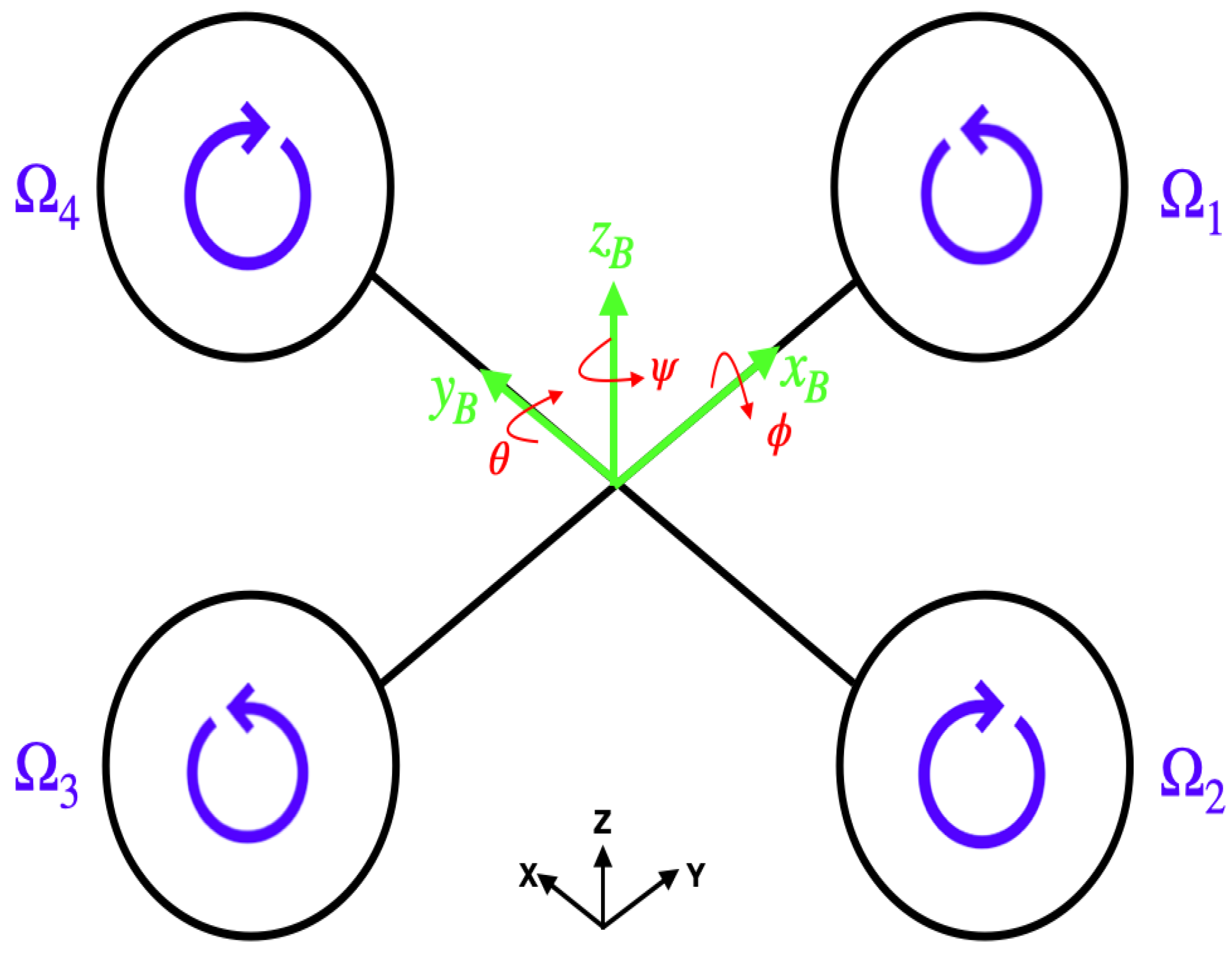
2. Quadrotor Dynamics

The quadrotor is composed of two main features: the body frame and the propellers. The function of the propellers is to give thrust to the UAV and to steer the quadrotor. The dynamics of the quadrotor are defined by the translation of the body in the XYZ space and the attitude of the body, which is composed of the rotational angles: roll, pitch, and yaw. Figure 1 presents a schematic of the quadrotor.
As seen in Figure 1, the propellers rotate in cross directions; if all the propellers rotate at the same speed and there is no external disturbance, the quadrotor will stay in a hovering state. The roll ϕ , pitch θ , and yaw ψ represent the rotational angles along the x B , y B and, z B -axes of the quadrotor respectively. [ Ω 1 , Ω 2 , Ω 3 , Ω 4 ] represent the velocity of each propeller. Note that the x B , y B and, z B -axes of the quadrotor are different from the XYZ axes defined by the Earth frame shown in black in Figure 1. To define the dynamics of the quadrotor, the equations will be divided into the Earth frame (E-frame) equations and the body frame (B-frame) equations, as shown in [30]. Afterward, both frames will be combined in a compound frame (C-frame).

2.1. E-Frame Dynamics

The E-frame dynamics are related to the movement of the center of gravity (COG) of the quadrotor with respect to an arbitrary origin set on a point of the Earth. These movements are the translation of the drone and are defined by the position, velocity, and acceleration of the quadrotor and the roll, pitch, and yaw movements. The set of equations used to describe the translation of the quadrotor is shown in Equation (1):
x ˙ = cos θ cos ψ u + ( sin ϕ sin θ cos ψ cos ϕ sin ψ ) v + ( cos ϕ cos θ cos ψ + sin ϕ sin ψ ) w y ˙ = cos θ sin ψ u + ( sin ϕ sin θ sin ψ + cos ϕ cos ψ ) v + ( cos ϕ sin θ sin ψ sin ϕ cos ψ ) w z ˙ = sin θ u + sin ϕ sin θ v + cos ϕ cos θ w ϕ ˙ = p + sin ϕ tan θ q + cos ϕ tan θ r θ ˙ = cos ϕ q sin ϕ r ψ ˙ = sin ϕ c o s θ q + cos ϕ c o s θ r
in which [ u , v , w ] is the velocity vector, while [ p , q , r ] is the angular velocity vector with respect to the B-frame. As seen in Equation (1), this representation is not enough to model the whole quadrotor because the previous equation is dependent on parameters defined in the body frame.

2.2. B-Frame Dynamics

In the B-frame, the origin is located at the COG of the quadrotor and moves with it. This type of representation is useful to see the effects that the rotation of each propeller generates at the quadrotor. Equation (2) shows the set of equations needed to represent these dynamics, including the gravitational term, the gyroscopic effect, and the input effect on these dynamics.
u ˙ = v r w q + sin θ g v ˙ = w p u r sin ϕ cos θ g w ˙ = u q v p cos ϕ cos θ g + U 1 m p ˙ = 1 J x x [ ( J z z J y y ) q r J p q Ω p + U 2 ] q ˙ = 1 J y y [ ( J z z J x x ) p r J p p Ω p + U 3 ] r ˙ = 1 J z z [ ( J y y J x x ) p q + U 4 ]
in which g is the gravitational constant; m is the mass of the quadrotor; [ J x x , J y y , J z z ] are the inertia tensor; and [ U 1 , U 2 , U 3 , U 4 ] are the auxiliary control inputs being functions of the speed of each rotor and defined by Equation (3)
U 1 = b ( Ω 1 2 + Ω 2 2 + Ω 3 2 + Ω 4 2 ) U 2 = b l ( Ω 4 2 Ω 2 2 ) U 3 = b l ( Ω 3 2 Ω 1 2 ) U 4 = d ( Ω 1 2 + Ω 2 2 Ω 3 2 + Ω 4 2 )
where b represents the thrust factor, l is the distance from the center of the quadrotor to the propeller, and d is the drag factor. The overall velocity of the propellers is defined as Ω p = Ω 1 + Ω 2 Ω 3 + Ω 4 .
Similar to the E-frame, the B-frame is not enough to understand all the dynamics of the quadrotor due to the dependence on parameters represented in the E-frame such as the roll, pitch, and yaw values. In order to build a model that includes all the dynamics of both the E-frame and the B-frame, a compound frame (C-frame) needs to be developed.

2.3. C-Frame Dynamics

In order to define a compound frame, a relation between the B-frame and the E-frame needs to be obtained. The relation of these two frames is represented by Equation (4).
ζ ˙ = J Θ v
in which ζ = [ x , y , z , ϕ , θ , ψ ] T is the E-frame vector; v = [ u , v , w , p , q , r ] T is the B-frame vector; and J Θ is a transformation matrix defined as:
J Θ = cos θ cos ψ sin ϕ sin θ cos ψ cos ϕ sin ψ cos ϕ sin θ cos ψ + sin ϕ sin ψ 0 0 0 cos θ sin ψ sin ϕ sin θ sin ψ + cos ϕ cos ψ cos ϕ sin θ sin ψ sin ϕ cos ψ 0 0 0 sin θ sin ϕ sin θ cos ϕ cos θ 0 0 0 0 0 0 1 sin ϕ tan θ cos ϕ tan θ 0 0 0 0 cos ϕ sin ϕ 0 0 0 0 sin ϕ cos θ cos ϕ cos θ
With this transformation matrix and Equations (1)–(4), the equations defining the dynamics of the quadrotor can be derived. These equations are shown in Equation (5).
x ¨ = 1 m [ cos ( ϕ ) sin ( θ ) cos ( ψ ) + sin ( ϕ ) sin ( ψ ) ] U 1 y ¨ = 1 m [ cos ( ϕ ) sin ( θ ) sin ( ψ ) sin ( ϕ ) cos ( ψ ) ] U 1 z ¨ = 1 m [ cos ( ϕ ) cos ( θ ) ] U 1 g p ˙ = 1 J x x [ ( J z z J y y ) q r J p q Ω p + U 2 ] q ˙ = 1 J y y [ ( J z z J x x ) p r J p p Ω p + U 3 ] r ˙ = 1 J z z [ ( J y y J x x ) p q + U 4 ]

3. LPV State Space Model of the Quadrotor

In order to build the MPC cost function, an LPV-state-space model with scheduling variable-dependent matrices A and B is defined. Using Equations (1)–(5), a nonlinear state-space model to track all the variables for the movement of the quadrotor can be derived. The nonlinear state-space model for the quadrotor is shown in Equation (6).
x ˙ = v x y ˙ = v y z ˙ = v z v ˙ x = 1 m [ cos ( ϕ ) sin ( θ ) cos ( ψ ) + sin ( ϕ ) sin ( ψ ) ] U 1 v ˙ y = 1 m [ cos ( ϕ ) sin ( θ ) sin ( ψ ) sin ( ϕ ) cos ( ψ ) ] U 1 v ˙ z = 1 m [ cos ( ϕ ) cos ( θ ) ] U 1 g ϕ ˙ = p + sin ( ϕ ) tan ( θ ) q + cos ( ϕ ) tan ( θ ) r θ ˙ = cos ( ϕ ) q sin ( ϕ ) r ψ ˙ = sin ( ϕ ) cos ( θ ) q + cos ( ϕ ) cos ( θ ) r p ˙ = 1 J x x [ ( J z z J y y ) q r J p q Ω p + U 2 ] q ˙ = 1 J y y [ ( J z z J x x ) p r J p p Ω p + U 3 ] r ˙ = 1 J z z [ ( J y y J x x ) p q + U 4 ]
As seen in the previous state-space system, the quadrotor is highly nonlinear; therefore, in order to treat the system as a linear state-space system, an LPV representation with six different scheduling variables depending directly on the states of the system is derived. The scheduling variables are presented in Equation (7).
ρ 1 = ϕ ρ 2 = θ ρ 3 = ψ ρ 4 = p ρ 5 = q ρ 6 = Ω p
The scheduling variables were chosen to represent the nonlinear state-space system of the quadrotor in an LPV state-space model using the least amount of scheduling variables needed to model the nonlinear dynamics of the quadrotor. With Equations (6) and (7), a quasi-LPV state-space system can be used to compute the MPC cost function in a linear form. The qLPV-SS with matrices A and B being scheduling parameter-dependent is shown in Equation (8).
x ˙ ( t ) = A ( ρ 1 , ρ 2 , ρ 3 , ρ 4 , ρ 5 , ρ 6 ) x ( t ) + B ( ρ 1 , ρ 2 , ρ 3 ) u ( t ) g
where x ( t ) = [ x , y , z , v x , v y , v z , ϕ , θ , ψ , p , q , r ] T , u ( t ) = [ U 1 , U 2 , U 3 , U 4 ] T , and matrices A and B are defined as follows:
A = 0 0 0 1 0 0 0 0 0 0 0 0 0 0 0 0 1 0 0 0 0 0 0 0 0 0 0 0 0 1 0 0 0 0 0 0 0 0 0 0 0 0 0 ϵ ρ 2 ϵ ρ 3 0 0 0 0 0 0 0 0 0 ϵ ρ 1 0 ϵ ρ 3 0 0 0 0 0 0 0 0 0 ϵ ρ 1 ϵ ρ 2 0 0 0 0 0 0 0 0 0 0 0 0 0 1 sin ( ρ 1 ) tan ( ρ 2 ) cos ( ρ 1 ) tan ( ρ 2 ) 0 0 0 0 0 0 0 0 0 0 cos ( ρ 1 ) sin ( ρ 1 ) 0 0 0 0 0 0 0 0 0 0 sin ( ρ 1 ) cos ( ρ 2 ) cos ( ρ 1 ) cos ( ρ 2 ) 0 0 0 0 0 0 0 0 0 0 J p ρ 6 J x x ( J z z J y y ) ρ 5 J x x 0 0 0 0 0 0 0 0 0 J p ρ 6 J y y 0 ( J z z J x x ) ρ 4 J y y 0 0 0 0 0 0 0 0 0 0 ( J y y J x x ) ρ 4 J z z 0
B = 0 0 0 0 0 0 0 0 0 0 0 0 0 0 0 1 m [ cos ( ρ 1 ) sin ( ρ 2 ) cos ( ρ 3 ) + sin ( ρ 1 ) sin ( ρ 3 ) ] 0 0 0 0 1 m [ cos ( ρ 1 ) sin ( ρ 2 ) sin ( ρ 3 ) sin ( ρ 1 ) cos ( ρ 3 ) ] 0 0 0 0 1 m [ cos ( ρ 1 ) cos ( ρ 2 ) ] 0 0 0 1 0 0 0 0 0 0 0 0 0 0 0 0 0 0 0 0 1 J x x 0 0 0 0 0 1 J y y 0 0 0 0 0 1 J z z 0
The value of ϵ is defined as a very low constant (e.g., ϵ = 1 × 10 3 ) and is included for the system to be controllable and to avoid having three zero rows in the A matrix. The parameter ϵ is therefore added for the MPC to identify that, by changing the attitude angles, the acceleration on the XYZ plane will be affected, but the predicted trajectory will not be significantly affected due to the small value of ϵ . The inclusion of the six different scheduling variables on the qLPV state-space allows for expressing the highly nonlinear quadrotor system into a compact quasi-linear state-space system, which is updated at each sampling time depending on the values of the states and the speed of the propellers. This compact qLPV-SS representation simplifies the computation of the future states of the system along the prediction horizon and improves the construction of the MPC cost function without splitting the system into several sub-systems. The gravitational constant is treated as an uncontrollable input or disturbance, which is constant at every sampling instant. In the next section, the proposed qLPV-SS presented in (8) will be used to compute the MPC cost function and to solve the optimization problem to obtain the optimal set of control actions.

4. Model Predictive Control Based on the LPV Representation of the Quadrotor

To build an MPC based on an LPV model, the prediction of the future states along the prediction horizon N p is formulated considering not only the state matrices A and B but also the variations in the scheduling variables along the prediction horizon. Therefore, matrices A and B are not considered constant along the prediction horizon, and the values of these matrices need to be considered for each step of the horizon in order to consider the nonlinear behavior of the quadrotor. Thus, Equation (9) presents the i-steps ahead calculation of the states of the quadrotor.
x ( k + i | k ) = j = 0 i 1 A d ρ i ( k + j ) x ( k ) + s = 1 i 1 l = s i 1 A d ρ i ( k + l ) B d ρ i ( k + s 1 ) u ( k + s 1 ) g + B d ρ i ( k + i 1 ) u ( k + i 1 ) g
where A d ( ρ i ) and B d ( ρ i ) are the discrete matrices obtained from the continuous matrices A and B presented in Section 3 using sampling time T s and zero-order-hold (ZOH) discretization. These matrices are updated at every sampling instant k as the set of scheduling parameters ( ρ i ) are also updated at each iteration. The prediction of the future states is performed along the prediction horizon, from k to k + N p ; thus, Equation (9) can be expressed as a compact matrix form to calculate the values of the states in the prediction horizon, as shown in Equation (10).
X = Φ · x ( k ) + Ψ · U
where
X = x ( k + 1 | k ) x ( k + 2 | k ) : . x ( k + N p | k )
Φ ( k ) = A d ρ i ( k ) j = 0 1 A d ρ i ( k + j ) j = 0 N p 1 A d ρ i ( k + j )
Ψ ( k ) = B d ( ρ i ( k ) ) 0 n x · n u 0 n x · n u A d ( ρ i ( k + 1 ) ) B d ( ρ i ( k ) ) B d ( ρ i ( k + 1 ) ) 0 n x · n u A d ( ρ i ( k + 2 ) ) A d ( ρ i ( k + 1 ) ) B d ( ρ i ( k ) ) A d ( ρ i ( k + 2 ) ) B d ( ρ i ( k + 1 ) ) 0 n x · n u ( i = 1 N p 1 A d ( ρ i ( k + 1 ) ) ) B d ( ρ i ( k ) ) ( i = 1 N p 1 A d ( ρ i ( k + 2 ) ) ) B d ( ρ i ( k + 1 ) ) B d ( ρ i ( k + N p 1 ) )
U = u ( k ) g u ( k + 1 ) g : . u ( k + N p 1 ) g
where X R N p · n x , Φ R N p × n x · n x , Ψ R N p · n x × N p · n u and U R N p · ( n u + 1 ) , where n x represents the number of states and n u represents the number of controllable inputs of the quadrotor. With Equation (10), the computation of the future values of the states of the quadrotor is performed, and a cost function for trajectory tracking can be designed to make the quadrotor follow a specified trajectory and to minimize the effort of the propellers. The proposed cost function is the following:
J = ( X ( k ) X r ( k ) ) T Q ( X ( k ) X r ( k ) ) + ( U ( k ) U ( k 1 ) ) T R ( U ( k ) U ( k 1 ) )
where Q R n x · N p × n x · N p and R R n u · N p × n u · N p are weighting matrices, X r is the trajectory reference vector along the prediction horizon, and U ( k 1 ) is the previous set of optimal control actions. For this application, the trajectory reference vector only includes the desired trajectory in the XYZ coordinates and the yaw angle reference. The other states are considered free states and are only bonded by the constraint limits. The values of the scheduling variables along the prediction horizon are calculated by using Equation (10) from the previous iteration. Having the future values of the states along the prediction horizon allows us to represent the nonlinear behavior of the quadrotor correctly in the MPC algorithm. The objective of the MPC strategy is to minimize the cost function (15) at every sampling instant k subject to the constraints shown in (16) and (17).
U m i n U U m a x
X m i n X X m a x
where U m i n , U m a x R ( n u + 1 ) · N p and X m i n , X m a x R n x · N p are the defined limits for the controlled inputs and the states, respectively. The gravitational term g included in the control vector U is constrained to be equal to 9.81 at every iteration. Thus, the optimization problem to solve at each sampling instant k is presented in Equation (18).
min U J s . t . ( 16 )   and   ( 17 )
Solving the optimization problem (18) results in the optimal set of control actions U along the prediction horizons; therefore, a conversion from the control actions to the actual speeds of the propellers that are input to the system needs to be performed. Using Equation (3), the values of the speed of each propeller can be calculated as shown in Equation (19).
Ω 1 2 Ω 2 2 Ω 3 2 Ω 4 2 = b b b b 0 b l 0 b l b l 0 b l 0 d d d d 1 U 1 U 2 U 3 U 4
To obtain the optimal velocities of each propellers [ Ω 1 , Ω 2 , Ω 3 , Ω 4 ] T , the absolute value of the square root of each square velocity is computed. Figure 2 presents the qLPV-MPC control strategy for the quadrotor using a compact 12-state qLPV system.

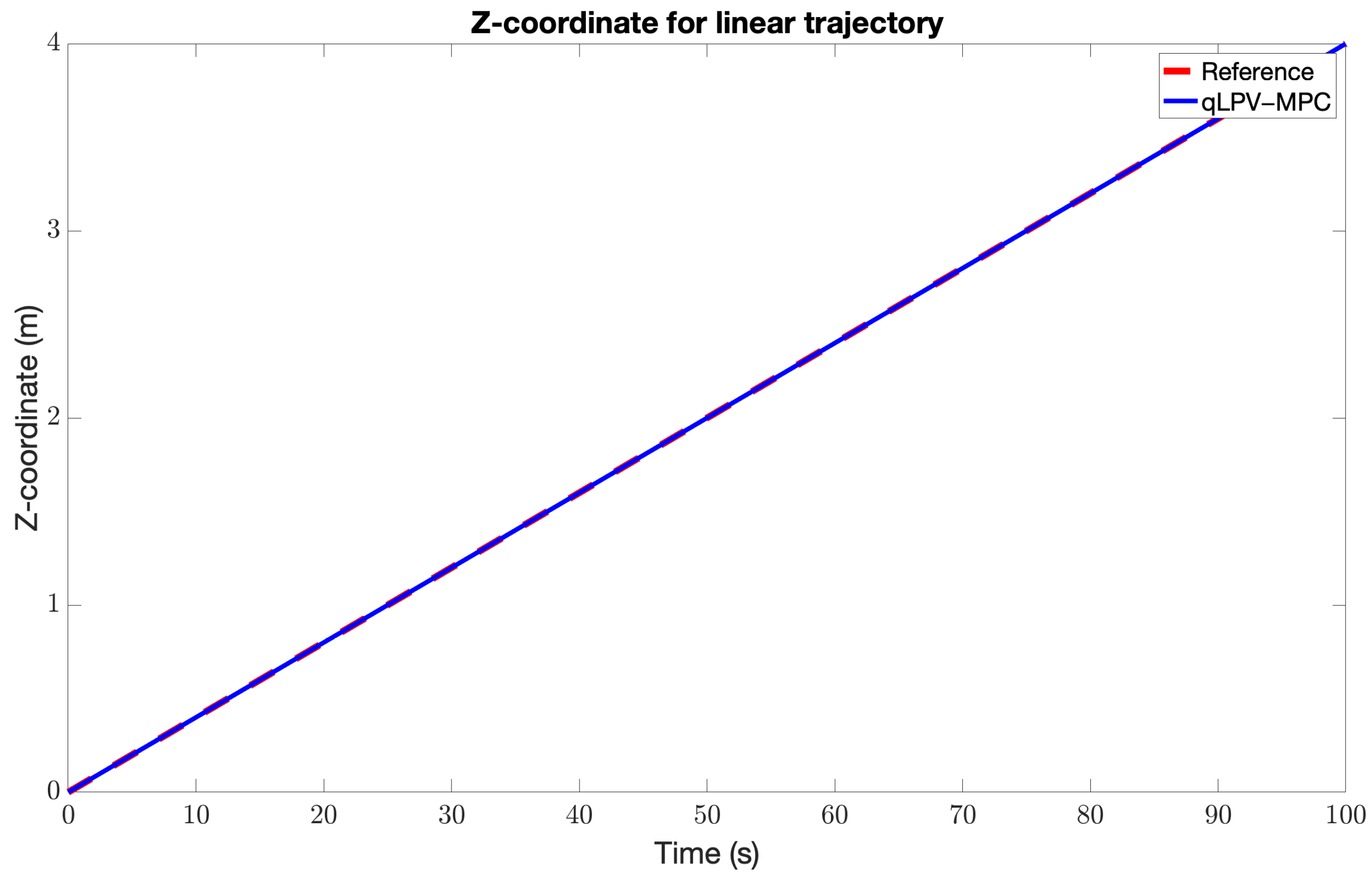
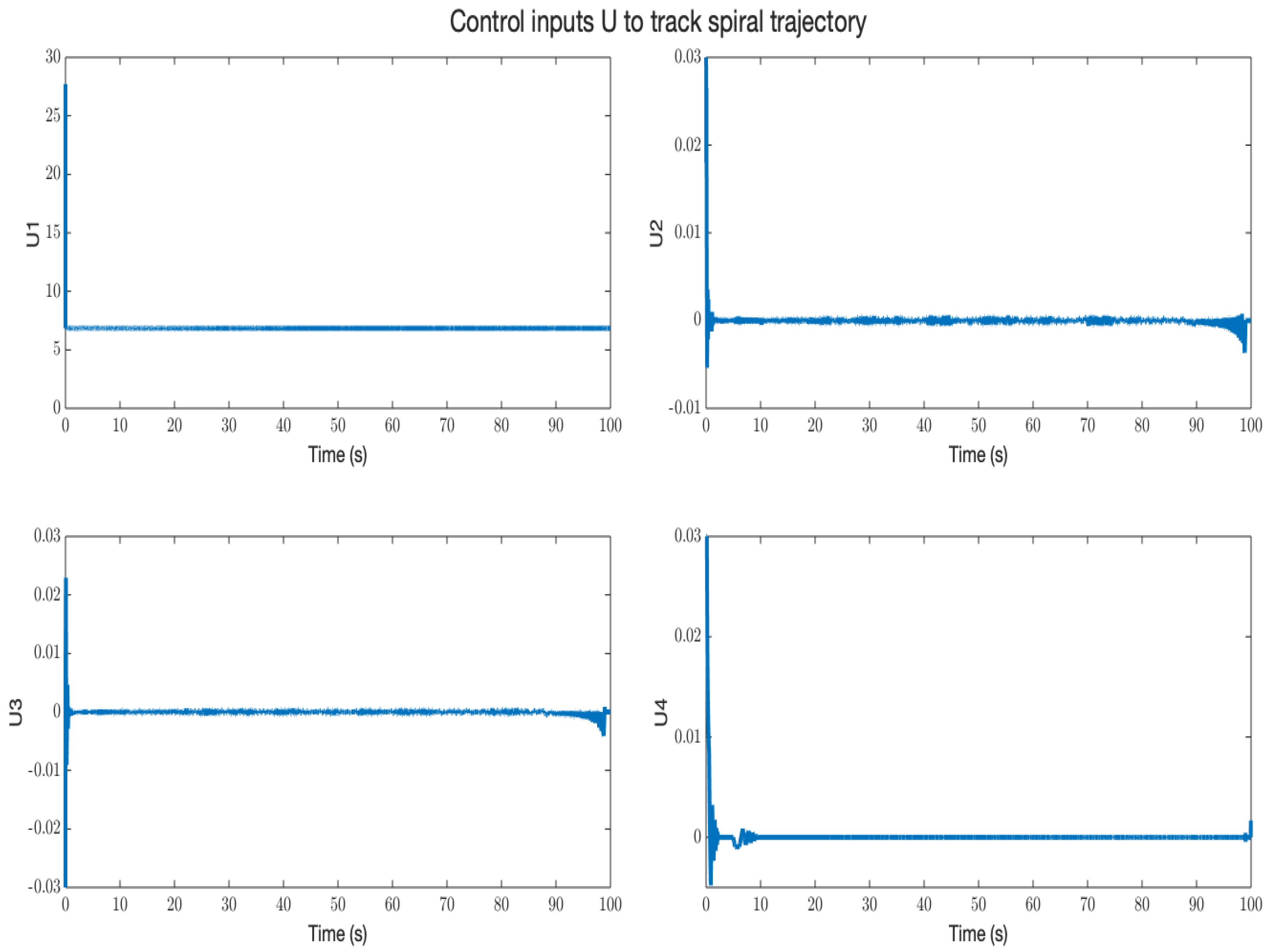
5. Results and Discussion

In order to test the performance of the proposed qLPV-MPC control strategy, a simulation of a quadrotor following two different trajectories will be performed. In the first test, a linear trajectory will be tested, while in the second test, the quadrotor will follow a spiral trajectory. In both tests, the quadrotor will start at a different starting point and will need to track and follow the trajectory. Table 1 shows the specifications of the quadrotor as presented in [26].
The linear trajectory and the spiral trajectory are shown in Figure 3 and Figure 4, respectively. The simulations were performed in the Matlab-Simulink (Matlab R2019b) software environment running on a Macbook Air with a dual-core Intel Core i5 1.8 GHz processor and 8 GB of RAM with 1600 MHz DDR3. The sampling time was set to T s = 10 ms to be able to measure and detect the fast dynamics of the quadrotor in any flying situation. The weighting matrix Q was designed in order to penalize the states more regarding the XYZ position and velocity at the first prediction steps. Weighting matrix R is designed as an identity matrix in order to penalize all the control actions equally. The optimization was performed using the Matlab function fmincon with the solver of sequential quadratic programming (SQP) to manage the cost function as a Quadratic Programming (QP) problem.
A prediction horizon of N p = 5 was defined after several simulations testing the performance for different prediction horizons. Increasing the prediction horizon will not improve the performance of the proposed control strategy significantly but will increase the optimization times, making real-time implementation impossible. Figure 5 presents the results of the trajectory tracking for the proposed qLPV-MPC for the linear reference trajectory. Figure 6, Figure 7 and Figure 8 show the values of the XYZ reference coordinates individually and the tracking carried out by the quadrotor with the qLPV-MPC strategy.
Figure 9 shows the behavior of the linear velocity in each coordinate and the angular position of the quadrotor during the tracking of the linear trajectory, while Figure 10 and Figure 11 show the control actions chosen and the required speed for each propeller.
Figure 12 presents the results of the trajectory tracking for the proposed qLPV-MPC for the linear reference trajectory. Figure 13, Figure 14 and Figure 15 show the values of the XYZ reference coordinates individually and the tracking performed by the quadrotor with the qLPV-MPC strategy.
Figure 16 shows the behavior of the linear velocity in each coordinate and the angular position of the quadrotor during the tracking of the linear trajectory, while Figure 17 and Figure 18 show the control actions chosen and the required speed for each propeller.
The control actions U present a small jitter, as shown in Figure 10 and Figure 17, as the nonlinearities of the system rapidly change the dynamics in the qLPV system; however, the speed of the rotors Ω , which are the physical control actions, do not present this behavior and make small variations to guide the drone to the desired trajectory. The performance of the proposed qLPV-MPC control for trajectory tracking of the quadrotor proved to be appropriate for tracking both the linear and the spiral trajectory even when starting at a different initial point. The qLPV-MPC plans an optimal trajectory for the quadrotor to be incorporated into the setpoint trajectory in the XYZ coordinates without trying to reach a point in the trajectory that will be unfeasible due to the constraints in both the states and the inputs, resulting in a smooth transition to the desired trajectory. As a result of this smooth transition, the quadrotor attack angles remain at small values, in order to avoid the instability of the UAV. It is also important to note that when the starting point of the quadrotor is also the starting point of the desired trajectory, the path tracking is performed perfectly, and the reference curves and the actual trajectory overlap each other even with nonlinear changes in the reference. This is an advantage of the MPC control strategy over other classical controllers that react over the tracking error.
The proposed controller also exhibits fast execution times, with an average time of 6.14 ms per optimization each iteration, and a worst-case time of 8.76 ms using the Matlab function ’fmincon’. Therefore, the proposed qLPV-MPC allows real-time implementation for the quadrotor with a sampling time of T s = 10 ms.

6. Conclusions

In this research work, a novel qLPV-MPC control strategy for a quadrotor based on a compact 12-state-space system is presented. The MPC controller is based on a qLPV system with six different scheduling parameters being states of the nonlinear quadrotor system in order to allow real-time implementation by solving the optimization problem in a short time. The prediction of the states along the prediction horizon is used in the next iterations to update the prediction matrices Φ and Ψ to model the nonlinear behavior of the quadrotor system by means of the scheduling variables. The proposed qLPV-MPC control strategy was tested by following two different trajectories, a linear trajectory, and a spiral trajectory. The results showed proper tracking of both trajectories while maintaining small roll, pitch, and yaw angles to maintain the quadrotor in a stable state. The execution times averaged 6.14 ms per optimization of each iteration which allows real-time implementation of the control strategy for the chosen sampling time of 10 ms. Future research work will focus on the robustness conditions of the proposed algorithm in the presence of wind disturbance and obstacle avoidance when following a desired path. An experimental test using a real quadrotor is also considered for future work.

Author Contributions

All authors (D.R.-G., A.F.-C., and O.J.G.-V.) have contributed as follows: Conceptualization, D.R.-G., A.F.-C., and O.J.G.-V.; Methodology, D.R.-G., A.F.-C., and O.J.G.-V.; Software, D.R.-G. and O.J.G.-V.; Validation, D.R.-G., A.F.-C., and O.J.G.-V.; Formal analysis, D.R.-G., A.F.-C., and O.J.G.-V.; Investigation, D.R.-G., A.F.-C., and O.J.G.-V.; Writing—original draft preparation, D.R.-G. and A.F.-C.; Writing—review and editing, D.R.-G., A.F.-C., and O.J.G.-V.; supervision, A.F.-C.; project administration A.F.-C. All authors have read and agreed to the published version of the manuscript.

Funding

This research received no external funding.

Institutional Review Board Statement

Not applicable.

Informed Consent Statement

Not applicable.

Data Availability Statement

No new data were created or analyzed in this study. Data sharing is not applicable to this article.

Acknowledgments

The authors thank Consejo Nacional de Ciencia y Tecnología (CONACyT) and Tecnológico de Monterrey for the financial support. Additionally, thanks go to the Nano-sensors from the School of Engineering and Sciences of Tecnológico de Monterrey for the support given to develop this work.

Conflicts of Interest

The authors declare no conflict of interest.

References

  1. Moreno-Valenzuela, J.; Pérez-Alcocer, R.; Guerrero-Medina, M.; Dzul, A. Nonlinear PID-type controller for quadrotor trajectory tracking. IEEE/ASME Trans. Mechatron. 2018, 23, 2436–2447. [Google Scholar] [CrossRef]
  2. Abdelhay, S.; Zakriti, A. Modeling of a quadcopter trajectory tracking system using PID controller. Procedia Manuf. 2019, 32, 564–571. [Google Scholar] [CrossRef]
  3. Idres, M.; Mustapha, O.; Okasha, M. Quadrotor trajectory tracking using PID cascade control. In IOP Conference Series: Materials Science and Engineering; IOP Publishing: Bristol, UK, 2017; Volume 270, p. 012010. [Google Scholar]
  4. El Hamidi, K.; Mjahed, M.; El Kari, A.; Ayad, H. Neural network and fuzzy-logic-based self-tuning PID control for quadcopter path tracking. Stud. Inform. Control 2019, 28, 401–412. [Google Scholar] [CrossRef]
  5. Minh, L.D.; Ha, C. Modeling and Control of Quadrotor MAV Using Vision-Based Measurement. In Proceedings of the International Forum on Strategic Technology (IFOST), Ulsan, Republic of Korea, 13–15 October 2010; pp. 70–75. [Google Scholar]
  6. Fessi, R.; Bouallègue, S. LQG controller design for a quadrotor UAV based on particle swarm optimisation. Int. J. Autom. Control 2019, 13, 569–594. [Google Scholar] [CrossRef]
  7. Bouselima, E.; Ichalal, D.; Mammar, S. Quadrotor Control and Actuator Fault Detection: LQG Versus Robust H-/H observer. In Proceedings of the 2019 4th Conference on Control and Fault Tolerant Systems (SysTol), Casablanca, Morocco, 18–20 September 2019; IEEE: Piscataway, NJ, USA, 2019; pp. 86–91. [Google Scholar]
  8. Emam, M.; Fakharian, A. Attitude tracking of quadrotor UAV via mixed H2/H∞ controller: An LMI based approach. In Proceedings of the 2016 24th Mediterranean Conference on Control and Automation (MED), Athens, Greece, 21–24 June 2016; IEEE: Piscataway, NJ, USA, 2016; pp. 390–395. [Google Scholar]
  9. Guo, M.; Su, Y.; Gu, D. Mixed H2/H∞ tracking control with constraints for single quadcopter carrying a cable-suspended payload. IFAC-PapersOnLine 2017, 50, 4869–4874. [Google Scholar] [CrossRef] [Green Version]
  10. Jasim, W.; Gu, D. H∞ path tracking control for quadrotors based on quaternion representation. In Advances in Autonomous Robotics Systems, Proceedings of the 15th Annual Conference, TAROS 2014, Birmingham, UK, 1–3 September 2014; Proceedings 15; Springer International Publishing: Berlin/Heidelberg, Germany, 2014; pp. 72–84. [Google Scholar]
  11. Kayacan, E.; Maslim, R. Type-2 fuzzy logic trajectory tracking control of quadrotor VTOL aircraft with elliptic membership functions. IEEE/ASME Trans. Mechatron. 2016, 22, 339–348. [Google Scholar] [CrossRef]
  12. Prayitno, A.; Indrawati, V.; Utomo, G. Trajectory tracking of AR. Drone quadrotor using fuzzy logic controller. TELKOMNIKA (Telecommun. Comput. Electron. Control) 2014, 12, 819–828. [Google Scholar] [CrossRef] [Green Version]
  13. Zhang, C.; Zhou, X.; Zhao, H.; Dai, A.; Zhou, H. Three-dimensional fuzzy control of mini quadrotor UAV trajectory tracking under impact of wind disturbance. In Proceedings of the 2016 International Conference on Advanced Mechatronic Systems (ICAMechS), Melbourne, VIC, Australia, 30 November–3 December 2016; IEEE: Piscataway, NJ, USA, 2016; pp. 372–377. [Google Scholar]
  14. Zhou, L.; Zhang, J.; Dou, J.; Wen, B. A fuzzy adaptive backstepping control based on mass observer for trajectory tracking of a quadrotor UAV. Int. J. Adapt. Control Signal Process. 2018, 32, 1675–1693. [Google Scholar] [CrossRef]
  15. Ganga, G.; Dharmana, M.M. MPC controller for trajectory tracking control of quadcopter. In Proceedings of the 2017 International Conference on Circuit, Power and Computing Technologies (ICCPCT), Kollam, India, 20–21 April 2017; IEEE: Piscataway, NJ, USA, 2017; pp. 1–6. [Google Scholar]
  16. Eskandarpour, A.; Sharf, I. A constrained error-based MPC for path following of quadrotor with stability analysis. Nonlinear Dyn. 2020, 99, 899–918. [Google Scholar] [CrossRef]
  17. Benotsmane, R.; Reda, A.; Vásárhelyi, J. Model Predictive Control for Autonomous Quadrotor Trajectory Tracking. In Proceedings of the 2022 23rd International Carpathian Control Conference (ICCC), Sinaia, Romania, 29 May–1 June 2022; IEEE: Piscataway, NJ, USA, 2022; pp. 215–220. [Google Scholar]
  18. Abdolhosseini, M.; Zhang, Y.M.; Rabbath, C.A. Trajectory tracking with model predictive control for an unmanned quad-rotor helicopter: Theory and flight test results. In Intelligent Robotics and Applications, Proceedings of the 5th International Conference, ICIRA 2012, Montreal, QC, Canada, 3–5 October 2012; Springer: Berlin/Heidelberg, Germany, 2012; Part I 5; pp. 411–420. [Google Scholar]
  19. Huang, S.; Teo, R.S.H.; Tan, K.K. Collision avoidance of multi unmanned aerial vehicles: A review. Annu. Rev. Control 2019, 48, 147–164. [Google Scholar] [CrossRef]
  20. Wang, D.; Pan, Q.; Shi, Y.; Hu, J.; Zhao, C. Efficient nonlinear model predictive control for quadrotor trajectory tracking: Algorithms and experiment. IEEE Trans. Cybern. 2021, 51, 5057–5068. [Google Scholar] [CrossRef] [PubMed]
  21. Liu, C.; Lu, H.; Chen, W.H. An explicit MPC for quadrotor trajectory tracking. In Proceedings of the 2015 34th Chinese Control Conference (CCC), Hangzhou, China, 28–30 July 2015; IEEE: Piscataway, NJ, USA, 2015; pp. 4055–4060. [Google Scholar]
  22. Kapnopoulos, A.; Alexandridis, A. A cooperative particle swarm optimization approach for tuning an MPC-based quadrotor trajectory tracking scheme. Aerosp. Sci. Technol. 2022, 127, 107725. [Google Scholar] [CrossRef]
  23. Zhao, C.; Wang, D.; Hu, J.; Pan, Q. Nonlinear model predictive control-based guidance algorithm for quadrotor trajectory tracking with obstacle avoidance. J. Syst. Sci. Complex. 2021, 34, 1379–1400. [Google Scholar] [CrossRef]
  24. Guevara, B.S.; Recalde, L.F.; Varela-Aldás, J.; Andaluz, V.H.G.; Gandolfo, D.C.; Toibero, J.M. A Comparative Study between NMPC and Baseline Feedback Controllers for UAV Trajectory Tracking. Drones 2023, 7, 144. [Google Scholar] [CrossRef]
  25. Stastny, T.J.; Dash, A.; Siegwart, R. Nonlinear mpc for fixed-wing uav trajectory tracking: Implementation and flight experiments. In Proceedings of the AIAA Guidance, Navigation, and Control Conference, Grapevine, TX, USA, 9–13 January 2017; p. 1512. [Google Scholar]
  26. Misin, M.; Puig, V. LPV MPC control of an autonomous aerial vehicle. In Proceedings of the 2020 28th Mediterranean Conference on Control and Automation (MED), Saint-Raphael France, 15–18 September 2020; IEEE: Piscataway, NJ, USA, 2020; pp. 109–114. [Google Scholar]
  27. Cavanini, L.; Ippoliti, G.; Camacho, E.F. Model predictive control for a linear parameter varying model of an UAV. J. Intell. Robot. Syst. 2021, 101, 57. [Google Scholar] [CrossRef]
  28. Singh, B.K.; Kumar, A. Model predictive control using LPV approach for trajectory tracking of quadrotor UAV with external disturbances. Aircr. Eng. Aerosp. Technol. 2023, 95, 607–618. [Google Scholar] [CrossRef]
  29. Qu, S.; Zhu, G.; Su, W.; Swei, S.S.M. LPV Model-based Adaptive MPC of an eVTOL Aircraft During Tilt Transition Subject to Motor Failure. Int. J. Control Autom. Syst. 2023, 21, 339–349. [Google Scholar] [CrossRef]
  30. Rodríguez Hernández, X. LPV Predictive Control of a Quadrotor. Master’s Thesis, Universitat Politècnica de Catalunya, Barcelona, Spain, 2020. [Google Scholar]
Figure 1. Quadrotor Schematic.
Machines 11 00755 g001
Figure 2. Block diagram of the proposed qLPV-MPC control strategy for a nonlinear quadrotor.
Machines 11 00755 g002
Figure 3. Linear trajectory set as the reference for the first test.
Machines 11 00755 g003
Figure 4. Spiral trajectory set as the reference for the second test.
Machines 11 00755 g004
Figure 5. Tracking of the linear trajectory using the qLPV-MPC.
Machines 11 00755 g005
Figure 6. Tracking of the x-coordinate using the qLPV-MPC for linear reference.
Machines 11 00755 g006
Figure 7. Tracking of the y-coordinate using the qLPV-MPC for linear reference.
Machines 11 00755 g007
Figure 8. Tracking of the z-coordinate using the qLPV-MPC for linear reference.
Machines 11 00755 g008
Figure 9. Behavior of the linear velocity and angular position of the quadrotor for tracking the linear trajectory.
Machines 11 00755 g009
Figure 10. Control inputs U for linear trajectory tracking.
Machines 11 00755 g010
Figure 11. Speed of the propellers Ω for linear trajectory tracking.
Machines 11 00755 g011
Figure 12. Tracking of the spiral trajectory using the qLPV-MPC.
Machines 11 00755 g012
Figure 13. Tracking of the x-coordinate using the qLPV-MPC for spiral reference.
Machines 11 00755 g013
Figure 14. Tracking of the y-coordinate using the qLPV-MPC for spiral reference.
Machines 11 00755 g014
Figure 15. Tracking of the z-coordinate using the qLPV-MPC for spiral reference.
Machines 11 00755 g015
Figure 16. Behavior of the linear velocity and angular position of the quadrotor for tracking the spiral trajectory.
Machines 11 00755 g016
Figure 17. Control inputs U for spiral trajectory tracking.
Machines 11 00755 g017
Figure 18. Speed of the propellers Ω for spiral trajectory tracking.
Machines 11 00755 g018
Table 1. Constant Values of the quadrotor.
VariableValueUnits
g9.8m/s 2
m0.698kg
J x x 0.0034kg · m 2
J y y 0.0034kg · m 2
J z z 0.006kg · m 2
J p 1.302 × 10 6 kg · m 2
b7.6184 × 10 9 N · s 2
d2.6839 × 10 9 N · s 2
l0.171m
Disclaimer/Publisher’s Note: The statements, opinions and data contained in all publications are solely those of the individual author(s) and contributor(s) and not of MDPI and/or the editor(s). MDPI and/or the editor(s) disclaim responsibility for any injury to people or property resulting from any ideas, methods, instructions or products referred to in the content.

