Article

Adaptive Control Strategy for a Pumping System Using a Variable Frequency Drive

Department of Automation and Applied Informatics, Politehnica University of Timisoara, Vasile Parvan, 300223 Timisoara, Romania
*
Authors to whom correspondence should be addressed.
Machines 2023, 11(7), 688; https://doi.org/10.3390/machines11070688
Submission received: 30 May 2023 / Revised: 22 June 2023 / Accepted: 26 June 2023 / Published: 30 June 2023
(This article belongs to the Special Issue Nonlinear and Adaptive Control of Intelligent Machines)

Abstract

:
Currently, the most implemented solution for driving a pumping system (PS) at variable speed is using a variable frequency drive (VFD). Because most of the VFDs have integrated only one proportional-integral (PI) frequency controller whose parameters (proportional gain/the integration time) can be off-line tuned but cannot be changed during real-time operation, and many PS must operate in different regimes (at variable speed, variable flow rate, at variable pumping head or even at variable power, e.g., those powered by renewable energy sources), the adaptive control strategy proposed in this paper overcomes these problems with very good performances. The proposed adaptive control strategy uses only simple PI controllers for managing several operating regimes. The adaptive character is not ensured by re-tuning the PI controller parameters as in self-tuning controllers but by readjusting the control law through a change in the control loop depending on the controlled output of the process (pump speed, pump discharge, pumping head or absorbed power). The deviations of the mentioned controlled outputs from their referenced values are converted into electrical frequency error (the deviation of the current value from its reference), which is the regular input to the already tuned controller; therefore, no controller re-tuning is required.

1. Introduction

In recent decades, pumping systems (PSs) have evolved significantly through progressive modernization to reach greater efficiency in water exploitation and use. This has been achieved by integrating various modern solutions that have replaced the traditional ones (for example, gravity irrigation has been replaced by sprinkler or drip irrigation systems). A consequence of those methods consisted of a drastic increase in energy consumption [1]. For this reason, in recent years, the classic regulation systems of PSs (both the valves that regulated the pumping head and flow, as well as the star and delta starting of the induction motors that drove the centrifugal pumps) were replaced by electronic power solutions, being more energy efficient [2]. Nowadays, the most implemented commercial solution for driving PS at variable speed is using a variable frequency drive (VFD) [3]. Because most of the VFDs have integrated only one proportional-integral (PI) frequency controller whose parameters (proportional gain/integration time) can be off-line tuned but cannot be changed during real-time operation, the current paper proposes a nonlinear dynamical mathematical model for a PS driven by a VFD and an adaptive control strategy for switching between four different regimes of a PS during operation without re-tuning the controller parameters. The proposed control strategy can handle four operating regimes: at variable speed (angular velocity), at variable discharge (pumping flow), at variable pumping head (pressure) and for tracking a variable available power (tracking a fluctuating and intermittent power source such as the power produced by renewable energy conversion systems [1,4]).
The current work presents the nonlinear modelling, control and simulation of a high-power PS. It begins with a short description of the considered PS and its main components, followed by its mathematical model in Section 2. Section 3 presents the proposed adaptive control strategy, and in Section 4, the performance of the proposed control strategy is determined by analyzing several performance indicators during four simulations, wherein the pumping system operates at desired variable speed, flow, pressure, and power. Section 5 presents the conclusions.
The main contribution brought by the current paper consists of the design, implementation and validation of a new adaptive control strategy for a pumping system using only simple PI controllers. The proposed adaptive control strategy is developed based on the vector control of an induction machine in the synchronous reference frame (“d-q”), whose references for the PI current controllers (one for the “d” axis and one for the “q” axis) are provided by other two PI controller in cascade, one for controlling the electrical frequency and one for controlling flux [1,5]. For switching between the different operating regimes of the PS, the speed error (the deviation of the current value from its reference), the pumping flow error, the pumping head error and the available power error are converted into electrical frequency error. The adaptive character is not ensured by re-tuning the PI controller parameters as in self-tuning controllers [6,7] or by a reference model [8,9] but by readjusting the control law through a change in the control loop depending on the controlled output of the process (pump speed, pump discharge, pumping head or absorbed power). The deviations of the mentioned controlled outputs from their referenced values are converted into electrical frequency error (the deviation of the current value from its reference), which is the regular input to the already tuned controller; therefore, no controller re-tuning is required.
The case studies, carried out through simulation in MATLAB and Simulink, considering an existing industrial high-power PS (whose layout is presented in Figure 1), led to the conclusion that the proposed adaptive control strategy ensures good performance, being recommended for PS configurations with induction motors driven by VFD with at least one integrated PI frequency controller (whose parameters can be programmable), that requires a switch between the different regimes during operation.
The considered PS is located in the Aragon region of Spain [10]. Figure 1 presents its layout and main components: a VFD that drives the induction motor of a submersible pump to collect water from a borehole and discharge it into a hydraulic distribution network.

2. Mathematical Model of a Pumping System Driven by a Variable Frequency Drive

In the current section, a nonlinear mathematical model of the considered high-power PS is developed. Figure 2 presents the diagram of the centrifugal pump driven by an induction motor powered by a constant and stable power source through a VFD [11]. According to Figure 2, through the VFD, the induction motor is driven at variable frequency, operating the centrifugal pump at variable speed, variable flow, variable pressure or at variable available power.
The nonlinear mathematical model mainly considered a variable frequency drive, an induction motor (IM), the centrifugal pump and the water distribution network (Figure 2). The dynamics of the other systems were either ignored or indirectly transferred to the already modeled systems.
The dynamic of the PS is modelled according to the following Equation (1) of motion [12],
I p s · ω p s ˙ = T I M T p u m p
and is based on the difference between the torques of the pump (Tpump) and the induction motor (TIM), with Ips being the PS moment of inertia and ωps the angular velocity of the motor (pump) shaft.

2.1. Variable Frequency Drive (VFD) Model

Besides the controller, the VFD also contains the execution elements (the rectifier and the inverter). The efficiency of the motor drive is calculated in Equation (2) based on the nominal power (PVFDnominal), output power (PVFDoutput) and three experimental parameters identified in reference [1,10]: k0 representing no-load losses, k1 representing the losses according to the voltage drop across diodes and k2 representing the resistive losses [1,10,13].
η V F D = p p · k 0 + k 1 · p V F D o u t p u t + k 2 · p V F D o u t p u t 2
where p = PVFDoutput/PVFDnominal, with the PVFDoutput being the VFD output power.
The AC electrical power required (input) by the VFD is obtained in Equation (3):
P V F D i n p u t = P V F D o u t p u t / η d r i v e / η f i l t e r / η c a b l e s
where PVFDinput is the VFD input power, ηdrive is the induction motor drive efficiency, ηfilter is the DV/DT filter efficiency, and ηcables is the efficiency after the loss due to the voltage drop in the cables. Table A1 from Appendix A presents the technical parameters of the VFD [1,10,11].

2.2. Induction Motor Model

The three-phase induction motor drives the centrifugal pump, and it can be powered through a VFD by power sources such as the national grid and diesel or gasoline generators. In Table A2 from Appendix A, it can be seen the technical parameters of the induction motor that drives the submersible pump.
The electrical angular velocity ωIM represents the angular velocity of the induction motor shaft angular velocity ωps multiplied by the pole pairs of the machine pmotor, as shown in Equation (4) [14]:
ω I M = p m o t o r · ω p s
The synchronous speed of the induction motor stator ωss is calculated according to Equation (5) [15]:
ω s s = 60 · f s p m o t o r
where fs = 50 [Hz] is the grid frequency of the balanced three phases and pmotor = 3 represents the induction motor pairs of poles (6 poles).
The nonlinear dynamic model of the three-phase induction motor is developed considering an induction machine operating in the motor regime, where the space vector theory of the basic electric equations of the machines is applied. In the current work, the synchronous reference frame (d-q) that rotates at synchronous speed is considered [14].
The induction motor stator and rotor voltage are obtained in a synchronously rotating reference frame using the electromagnetic Equations (6) and (7) [16]:
v s a = R s · i s a + d ψ s a d t + j · ω s s · ψ s a > v d s = R s · i d s + d ψ d s d t ω s s · ψ q s v q s = R s · i q s + d ψ q s d t + ω s s · ψ d s
0 = R r · i r a + d ψ r a d t j · ω s s ω I M · ψ r a > 0 = R r · i d r + d ψ d r d t ω s s ω I M · ψ q r 0 = R s · i q r + d ψ q r d t + ω s s ω I M · ψ d r
where a denotes that the space vectors refer to a synchronously rotating reference frame; v s a is the stator voltage vector reference to a synchronously rotating frame; Rs and Rr are the stator and rotor resistances; i s a is the stator current vector reference to a synchronously rotating frame; d ψ s a is the stator flux vector reference to a synchronously rotating frame; vd and vq are the voltage vector d and q components; ψds and ψqs are the d and q components of the stator flux; ids and iqs are the d and q components of the stator current; idr and iqr are the d and q components of the rotor current; i r a is the rotor current vector reference to a synchronously rotating frame; ψ r a is the rotor flux vector reference to a synchronously rotating frame, and ψdr and ψqr are the d and q components of the rotor flux.
Similar to the voltage equations, the flux equations are obtained in a synchronously rotating reference frame using Equations (8) and (9) [15]:
ψ s a = L σ S + L m · i s a + L m · i r a > ψ d s = L σ S + L m · i d s + L m · i d s ψ q s = L σ S + L m · i q s + L m · i q s
ψ r a = L m · i s a + L σ r + L m · i r a > ψ d r = L m · i d r + L σ r + L m · i d r ψ q r = L m · i q s + L σ r + L m · i q r
where Lm is the magnetizing inductance, and Lσs and Lσr are the leakage inductances of the stator and rotor windings.
The active power of the induction motor PIM is calculated using Equation (10) [14]:
P I M = 3 2 · v d · i d + v q · i q
The reactive power of the induction motor QIM is calculated using Equation (11) [14]:
Q I M = 3 2 · v q · i d v d · i q
The electromagnetic torque of the induction motor TIM is calculated using Equation (12) [16]:
T I M = 3 2 · p m o t o r · L m L σ r + L m · ψ q s · i d r ψ d s · i q r T I M = 3 2 · p m o t o r · L m L σ r + L m · ψ s · i q r = k _ T · i q r
The diagram from Figure 3 represents the flow chart of the induction motor model developed in Simulink:

2.3. Variable Speed Centrifugal Pump Model

The variable-speed centrifugal pump [17] is a submersible pump that collects water from a well and delivers it directly into an irrigation hydraulic distribution network at different operating points. Besides the technical specifications, Table A3 in Appendix A also presents the operating points of the submersible pumps [17]. The variable-speed centrifugal pump is installed, below the lowest water level, at a depth of 40 m (PUMP_DEPTH ≈ 40 m below the ground level in Figure 1), and the water is extracted from a depth of 30.5 m (HG_WATER_SOURCE ≈ 30.5 m dynamic level in Figure 1). The pump discharges a nominal flow of 91.85 m3/h, with the maximum discharge being 95 m3/h.
The variable centrifugal pump is modelled based on A, B, C, D and E coefficients from Table 1.
The coefficients are identified through quadratic regression on seven operating points on the pump head–flow (H0-Q0) and efficiency–flow (η0-Q0) curves at 50 Hz provided by the manufacturer (Figure 4) using the nonlinear model developed and fully explained in [1] (same denotation as in reference [1] are also used in the current paper).
The centrifugal pump head-flow characteristic (Hs-Qs) is modeled as a function of pump speed according to Equation (13) from references [1]:
H s = ω p s s ω p s 0 2 · A + ω p s s ω p s 0 · B · Q s + C · Q s 2
The centrifugal pump efficiency is modeled as a function of pump speed according to Equation (14) from references [1]:
η s ω p s = 1 ω p s 0 ω p s s 0.1 + D · Q s · ω p s 0 ω p s s 1.1 + E · Q s 2 · ω p s 0 ω p s s 2.1
Figure 4a shows the pump characteristics head-flow (H-Q) curves (representing the pumping head in meters on the x-axis and the pump discharge in m3/h on the y-axis) at different electrical frequencies (variations from 5 to 50 Hz)—equivalent to the pump angular velocity.
Figure 4b shows the pump efficiencies (η-Q) curves (representing the pump efficiency on the x-axis and the pump discharge in m3/h on the y-axis) at different electrical frequencies (variations from 5 to 50 Hz).
By combining the head-flow (H-Q) characteristic curves of the pump, Equation (13), with the pump efficiency-flow (η-Q) characteristic curves from Equation (14), the iso-efficiency curves are obtained in Figure 5a. The pump efficiency is represented in percentages by the dotted lines, while the pump frequency is represented in Hz by the dashed lines. The red line represents the hydraulic (water distribution and irrigation system) network characteristic curve Hs(Qs) from Equation (18) (Section 2.4).
The pump iso-power curve is presented in Figure 5b, where the pump power (Ppump) is calculated based on delivered hydraulic power (Phydraulic) divided by the pump efficiency at the operating point (ηs), as shown in Equation (15) [18]:
P p u m p = P h y d r a u l i c η s = ρ w · g · H s · Q s η s
where ρw is the water density, and g is the gravitational acceleration.
The pump iso-torque curve is presented in Figure 5c, where the pump torque (Tpump) is calculated according to Equation (16) from reference [19]:
T p u m p = 60 · P p u m p 2 · π · ω p s s
The pump iso-inertia curve is presented in Figure 5d, where the pump inertia (Ips) is calculated based on Equation (17) [20]:
I p s = 0.03768 · P p u m p 1000 · ω p s s 0.9556

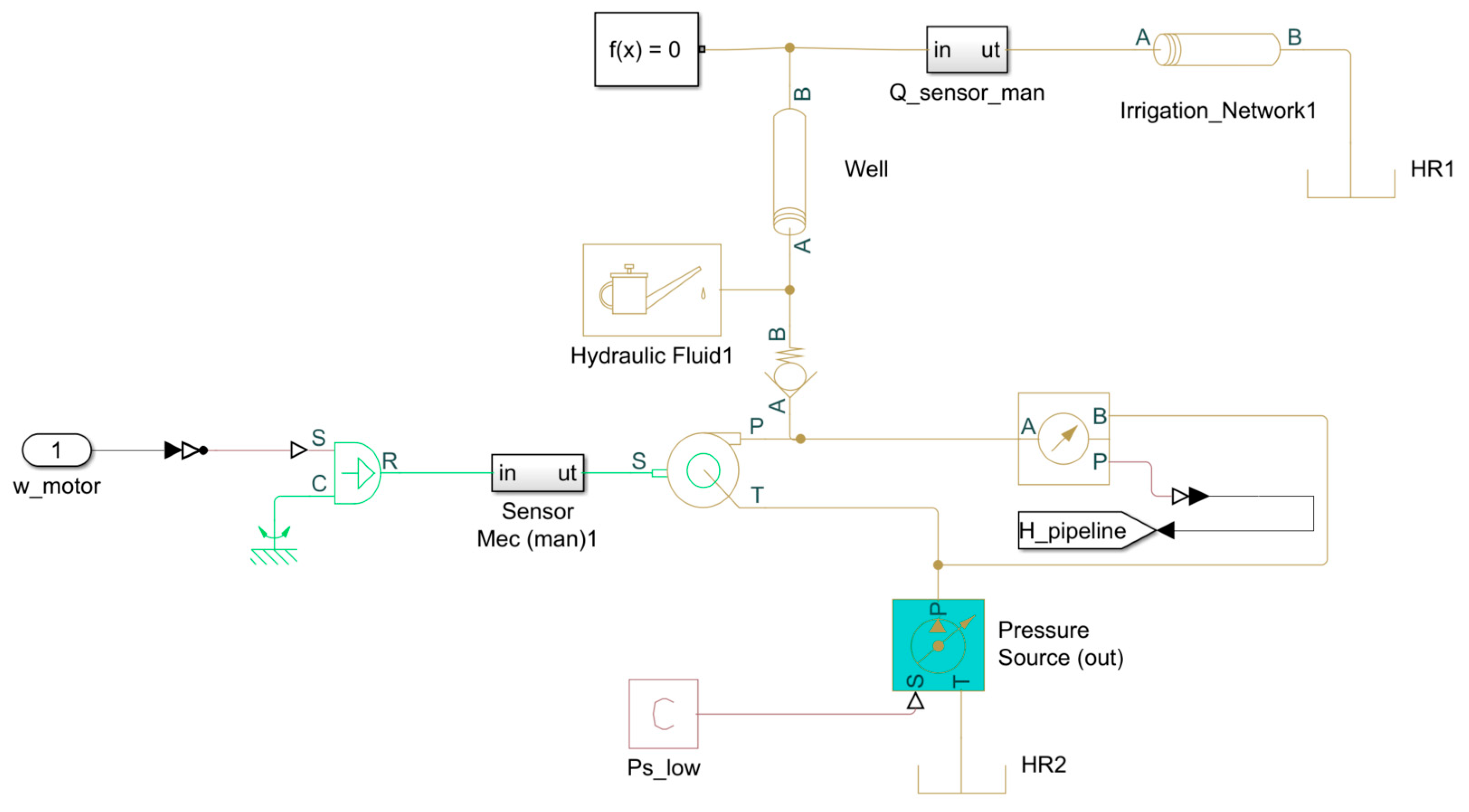
2.4. Hydraulic Network Model

The considered high-power PS presents five operating points. Table 2 presents the nominal values of the key parameters for each operating point obtained through sensor acquisition on the existing industrial high-power PS.
The water distribution and irrigation system characteristic curve is expressed by Equation (18) [21] and represented with the red line in Figure 5:
H s = H g + k · Q s 2
where Qs is the current pump discharge, Hg is the static head, and k is the head loss coefficient. Figure 5a shows the iso-efficiency diagram of the pump together with the hydraulic network characteristic curve [1].
The pump discharge (flow rate) as a function of pump speed (ωps0) is given by the cross-point of the pump head flow characteristic curve (Equation (13)) with the hydraulic network characteristic curve (Equation (18)), resulting in Equation (19):
Q s ω p s s = ω p s s ω p s 0 · B ω p s s ω p s 0 2 · B 2 4 · ω p s s ω p s 0 2 · A H g · C k 2 · C k
The pump power (Ppump) is calculated based on delivered hydraulic power (Phydraulic) divided by the pump efficiency at the operating point (ηs), Equation (20) [1]:
T p u m p = ρ w · g · H g · Q s + ρ · g · k 1 · Q s ω p s s 3 ω p s s · 1 ω p s 0 ω p s s 0.1 + D · Q s ω p s s · ω p s 0 ω p s s 1.1 + E · Q s ω p s s 2 · ω p s 0 ω p s s 2.1
The pump inertia (Ips) is calculated based on the following Equation (21) [20]:
I p u m p = 0.03768 · ρ w · g · H g · Q s + ρ · g · k 1 · Q s ω p s s 3 1 ω p s 0 ω p s s 0.1 + D · Q s ω p s s · ω p s 0 ω p s s 1.1 + E · Q s ω p s s 2 · ω p s 0 ω p s s 2.1 1000 · ω p s s 0.9556
Figure 6 presents the diagram of the centrifugal pump together with the hydraulic network implemented in Simulink.

3. The Proposed Adaptive Control Strategy

The most common solution for driving high-power centrifugal pumps at a variable speed is using a VFD that, by varying the frequency of the induction motor, varies the speed of the pump. Besides controlling the acceleration to the nominal frequency (0–50 Hz) and deceleration from the nominal frequency (50–0 Hz) of the induction motor, a VFD also controls the operation at a variable frequency that can differ from the nominal one (≠50 Hz).
Because most of the VFDs have integrated only one proportional-integral (PI) frequency controller whose parameters (proportional gain/the integration time) can be off-line tuned but cannot be changed during real-time operation, in the current section, an adaptive control strategy is developed, that allows switching between four different regimes of a PS during operation without changing the controller parameters: at variable speed (angular velocity), at variable discharge (pumping flow), at variable pumping head (pressure) and for tracking a variable available power (tracking a fluctuating and intermittent power source such as the power produced by renewable energy conversion systems [1,4]).
The commutation between the operating regimes is performed manually. However, each of these operating regimes implies an adaptation of the control law through an automatic change and recalculation of the electrical frequency error, which is the regular input to the already tuned controller; therefore, no controller re-tuning is required. Thus, the adaptive behavior consists of readjusting the control law through a change in the control loop depending on the controlled output of the process (pump speed, pump discharge, pumping head or absorbed power). In this way, no separate control systems are needed for each operating regime, the proposed unitary adaptive control strategy being able to manage all these regimes. Figure 7 shows this automatic adaptation of the deviations of the mentioned controlled outputs from their referenced values (depending on the selected operating mode), which leads to a change of the control law and implicitly to an adaptive control strategy. In this way, the error calculation block will always generate an electrical frequency error as an input which the controller can handle for any selected operating mode.
Figure 7 presents the VFD control loop block diagram in Simulink. Where the blue blocks, together with the orange block (the only PI regulator in the VFD control architecture that allows off-line tuning of its parameters but cannot be changed during real-time operation), represent the classical variable speed pump control loops implemented in the VFD. The purple blocks represent the mathematical equations (Equations (42) and (43)) with which the classical variable speed pump control loops were extended to operate the centrifugal pump at variable flow (pump discharge). The green blocks represent the mathematical equations (Equations (44) and (45)) with which the classical variable speed pump control loops were extended to operate the centrifugal pump at variable pressure (pumping head). The red blocks represent the mathematical equations (Equations (46) and (47)) with which the classical variable speed pump control loops were extended to operate the centrifugal pump at variable available power. Through the selection of the operating regime (Order_operating_regim input in Figure 7), the proposed control system adapts its strategy according to the desired operating regime by converting the pumping flow error (purple blocks in Figure 7), the pumping head error (green blocks in Figure 7), and the available power error (red blocks in Figure 7) into the electrical frequency error of the programable PI (orange block in Figure 7). The deviations from the pumping flow and head references are obtained by closing the feedback loops with the current values from the nonlinear model of the centrifugal pump together with the hydraulic network from Figure 6 (q_pipeline and H_pipline from Figure 7 are obtained from Q_sensor_main and H_pipline from Figure 6). The deviations from the induction motor speed and power are obtained by closing the feedback loops with the current values from the nonlinear model of the induction motor from Figure 3 (omega_pm and P_motor_pump from Figure 7 are obtained from omega_pm and the power meter from Figure 3).
Where [5,16]:
  • G1, G2 and G3 are variable gains obtained in Equations (43), (45) and (47);
  • k_T represents the torque coefficient calculated in Equation (12);
  • D Q d / q represents the transformation from a stationary (αβ) reference frame into a synchronous (dq) reference frame;
  • a b c D Q represents the transformation from a three-phase (abc) complex space vector into a stationary (αβ) reference frame;
  • d / q D Q represents the transformation from a synchronous (dq) reference frame into a stationary (αβ) reference frame;
  • D Q a b c represents the transformation from a stationary (αβ) reference frame into a three-phase (abc) complex space vector.
d / q D Q = cos θ s sin θ s sin θ s cos θ s ;   D Q d / q = cos θ s sin θ s sin θ s cos θ s ; D Q a b c = 1 0 1 / 2 3 / 2 1 / 2 3 / 2 ;   a b c D Q = 3 2 · 1 1 / 2 1 / 2 0 3 / 2 3 / 2 ;

3.1. Classical Variable Speed Pump Control Strategy Implemented in a VFD

The classical variable speed pump control strategy implemented in the VFD considers a classical solution for current regulation in vector-controlled AC drives. This solution contains two PI (Proportional Integral) controllers, one for the speed and one for the flux, connected in cascade with two equally tuned PI current regulators, one to control the “d”-axis currents and one for the “q”-axis currents. The two PI current regulators are equally tuned using a second-order equivalent system of induction motor currents (Equation (23)), as described in reference [1]:
s 2 + s · R S + k p 1 σ · L S + k i 1 σ · L S = s 2 + 2 · ξ 1 · ω n 1 · s + ω n 1 2
with σ being the leakage coefficient [10]:
σ = 1 L m 2 L s · L r
where Rs = 0.095 [Ω] represents the IM stator resistance, Rr = 0.063 [Ω] represents the IM rotor resistance, Lm = 0.032 [H] is the IM magnetizing inductance, Ls = 0.034 [H] being the IM stator inductance, and Lr = 0.034 [H] the IM rotor inductance. ωn1 and ξ1 are the first natural frequency and damping factors of the system. kp1 and ki1 are the proportional gain and integration time of both closed-loop current systems (“d” and “q”), as both PI current regulators are equally tuned.
From Equation (23), it results that the required proportional gain and integral time constant are as in Equations (25) and (26), respectively:
k p 1 = σ · L s · 2 · ξ 1 · ω n 1 R s
k i 1 = σ · L s · ω n 1 2
with a damping factor equal to 1, ξ1 = 1 [1]:
ξ 1 = 1   results   s + ω n 1 2
and
ω n 1 = 10 σ · L s R s
To the q-axis PI current regulator is added in cascade, a speed controller, that becomes the main loop. The speed controller provides the reference for the inner loop q-axis current (iqs*) containing the current regulation (q-axis) from the electromechanical torque according to Equation (12) from [16], resulting in Equation (29):
T e m * T e m = K · Ψ d r · i q s
which allows us to obtain the q-axis current reference, iqs*.
The synthesis of the speed controller is carried out, starting from Equation (30) [16], where the viscous friction has been neglected:
T e m T p u m p = I p u m p · ω p s s ˙ = 2 · π · I p s p m o t o r · f m ˙
and fm represents the electrical motor frequency in Equation (31) [1]:
f m = p m o t o r · ω p s s 2 · π
Ips represent the total inertia of the pumping unit (induction motor plus pump), Equation (21), and Tpump represents the mechanical torque (Equation (20)).
Denoting ΔT = TemTpump, from Equation (30), the following transfer function of the driving shaft system is obtained in Equation (32):
f m s T s = p m o t o r 2 · π · I p u m p · s
Considering the transfer function of a Proportional and Integral controller (PI2) of the form of Equation (33):
P I 2 = k p 2 + k i 2 s
in series with the transfer function from Equation (32), the transfer function of the closed loop with unitary feedback is obtained in Equation (34):
f m s f m * s = k p 2 · s + k i 2 2 · π p m o t o r · I p u m p · s 2 + k p 2 · s + k i 2
with fm* being the electrical motor frequency and representing the input and fm being the current motor electrical frequency and representing the output.
For tuning the PI2 speed controller, the closed loop denominator of Equation (34) is matched to the denominator of a standard second-order system in Equation (35):
s 2 · 2 · π · I p u m p / p m o t o r + s · k p 2 + k i 2 = s 2 + 2 · ξ 2 · ω n 2 · s + ω n 2 2
The required proportional gain (kp2) and integral time constant (ki2) are obtained in Equations (36) and (37):
k p 2 = 2 · ξ 2 · ω n 2 · p m o t o r 2 · π · I p
k i 2 = ω n 2 2 · p m o t o r 2 · π · I p
In parallel, a flux controller loop is developed and added in cascade to the d-axis PI current regulator, similar to the speed controller loop. The flux controller becomes the main loop and provides the reference for the inner loop d-axis current (ids*) containing the current regulation (d-axis).
The synthesis of the flux controller starts from the transfer function of the rotor flux estimator (Equation (38)) function from reference [14]:
Ψ d r s i d s s = L m τ r · s + 1
where the dynamics of the d-axis current control loop are neglected because the d-axis current loop dynamic is much faster than the rotor flux dynamic. τr represents the rotor time constant.
By including the transfer function of another PI regulator type, Equation (33), (PI3) in series with the rotor flux estimator and closing the loop with unitary feedback, the transfer function of the rotor flux closed loop is obtained:
Ψ d r s Ψ d r * s = k p 3 · s + k i 3 s 2 · τ r L m + s · 1 L m + k p 3 + k i 3
where the current rotor flux (Ψdr) is the output, and the reference of the rotor flux (Ψdr*) is the input.
The proportional gain kp3 and the integral time constant ki3 of the flux controller are obtained in Equations (40) and (41) from the identification of the closed-loop denominator of Equation (39) with a standard second-order system denominator:
k p 3 = τ r L m · ω n 3 2
k i 3 = τ r L m · 2 · ξ 3 · ω n 3 1 L m

3.2. Adapting the Variable Speed Pump Control Strategy of the VFD to Operate the Centrifugal Pump at Variable Flow (Pump Discharge)

A particular application of the variable speed pump is the pumping system that must operate at the desired water discharge (volume flow). Due to this reason, a mathematical equation is introduced (Equation (42)) to obtain the electrical frequency error ∆f = (fm*fm) expressed as a function of water discharge (flow) error ∆Q = (Q*Q), and the first-order Taylor series approximation is used:
Q = Q * + 2 · π p m o t o r · f m f m * · Q ˙ f m *
where Q ˙ is obtained deriving affinity laws from reference [19], the angular velocity (ωpss) is converted into electrical frequency (fm) (Equation (31)), and the nominal discharge (flow) (Q0) and frequency (fm0) are equal to the reference discharge (Q* = Q0) and frequency (fm* = fm0). From Equation (42), Equation (43) is obtained:
Q = 2 · π p m o t o r · f · Q ˙ f m * = 2 · π · Q * p m o t o r · f m * · f   and   f = p m o t o r · f m * 2 · π · H * · Q = G 1 · Q
The blocks and lines highlighted with purple in Figure 2 represent the diagram of the electrical connections to the VFD in order to operate the centrifugal pump at a referenced flow. G1 represents the variable gain used for converting the water discharge (flow) error into an electrical frequency error.

3.3. Adapting the Variable Speed Pump Control Strategy of the VFD to Operate the Centrifugal Pump at Variable Pressure (Pumping Head)

A particular application of the variable speed pump is the pumping system that must operate at the desired variable pressure (pumping head). Due to this reason, a mathematical equation is introduced (Equation (44)) to obtain the IM electrical frequency error ∆f = (fm*fm) as a function of pumping head error ∆H = (H*H), using the first-order Taylor series approximation:
H = H * + 2 · π p m o t o r · f m f m * · H ˙ f m *
where H ˙ is obtained deriving affinity laws from reference [19], the angular velocity (ωpss) is converted into electrical frequency (fm) (Equation (31)), and the nominal head (H0) and frequency (fm0) are equal with the reference head (H* = H0) and frequency (fm* = fm0) [1]. From Equation (44) results Equation (45):
H = 2 · π p m o t o r · f · H ˙ f m * = 4 · π · H * p m o t o r · f m * · f   and   f = p m o t o r · f m * 4 · π · H * · H = G 2 · H
The blocks and lines highlighted with green in Figure 2 represent the diagram of the electrical connections to the VFD in order to operate the centrifugal pump at a referenced pumping head. G2 represents the variable gain used for converting the pumping head (pressure) error into an electrical frequency error.

3.4. Adapting the Variable Speed Pump Control Strategy of the VFD to Operate the Centrifugal Pump at Variable Available Power (Tracking a Fluctuating and Intermittent Power Source)

A particular application of the variable speed pump is the pumping system that must operate at variable available power (tracking a fluctuating and intermittent power source). For example, in the pumping systems powered by a photovoltaic or electrical wind generator, where the pumping system absorption power must track the power produced by a photovoltaic (electrical wind) generator. Due to this reason, a mathematical equation is introduced (Equation (46)) to obtain the electrical frequency error ∆f = (fm*fm) expressed as a function of pump power error ∆Ppump = (Ppump*Ppump), and the first-order Taylor series approximation is used:
P p u m p = P p u m p * + 2 · π p m o t o r · f m f m * · P p u m p ˙ f m *
where P p u m p ˙ is obtained deriving affinity laws from reference [19], the angular velocity (ωpss) is converted into electrical frequency (fm) (Equation (31)), and the nominal pump power (Ppump0) and frequency (fm0) are equal with the reference pump power (Ppump* = Ppump0) and frequency (fm* = fm0). From Equation (46) results Equation (47):
P p u m p = 2 · π p m o t o r · f · P p u m p ˙ f m * = 4 · π · H * p m o t o r · f m * · f and f = p m o t o r · f m * 6 · π · P p u m p * · P p u m p = G 3 · P p u m p
The blocks and lines highlighted with red in Figure 2 represent the diagram of the electrical connections to the VFD in order to operate the pumping unit (centrifugal pump together with the induction motor) at a variable available power. G3 represents the variable gain used for converting the pump power error into an electrical frequency error.

4. Simulation Results

The proposed adaptive control strategy presented in Section 3 and the dynamic model of the pumping system described in Section 2 have been validated through simulation in Simulink. Four simulations were executed to analyze and evaluate the response of the pumping unit (induction motor plus centrifugal pump) driven by a VFD in four different regimes:
  • Variable speed;
  • Variable flow (pump discharge);
  • Variable pressure (pumping head);
  • Variable available power (tracking a fluctuating and intermittent power source).

4.1. Response of the Adaptive Control Strategy Operating the Centrifugal Pump at Variable Speed

The first simulation (12 s—Figure 8) presents the response of the pumping unit driven by a VFD (in the variable speed mode) by a reference speed step from 1800 rpm to 2400 rpm, occurring in the fourth second. In the ninth second, the proposed control strategy stops the pumping system operation.
In Figure 8, it can be seen that the developed strategy for controlling the pump to variable speed makes the pump seed reach its reference with a small overshoot (MP = 0.3761%) occurring at the peak time Tp = 0.9679 s after the step, with a settling time Ts = 1.0285 s (1% criterium) and a rise time of Tr = 0.7575 s (the time for the output to reach from 5% to 95% of the reference). Figure 9a presents the induction motor’s speed reference expressed in electromechanical torque, the actual electromechanical torque and the load (pump) torque. It can be seen that the proposed control strategy drives the induction motor with its maximum torque until it reaches the torque equivalent to its reference speed.
Figure 9b depicts the electrical power absorbed from the power grid, the motor electromechanical power, the mechanical (rotational) power provided by the motor and the pump’s shaft mechanical (rotational) power. During the power transition of the induction motor, the absorbed power from the grid will not exceed the nominal power of the motor. The fluctuations of the absorbed power do not exceed 1% (accepted by most of the power grids).
As seen in Figure 9c, the proposed adaptive control strategy holds constant the three phases of voltage supply from the power grid to the induction motor.
In Figure 9d, it can be seen the current variation of the three phases supplying the induction motor.
Figure 9e presents the pump water discharge (flow) variation during the variable speed step response.
In Figure 9f it can be seen the pumping head (pressure) variation during the variable speed step response. According to Figure 9f, it can be seen that during both speed steps, one from 1800 rpm to 2400 rpm in the fourth second and one from 2400 rpm to 0 rpm in the ninth second, no over or under pressure occurs that could lead to water hammer or cavitation in the pump [22,23].

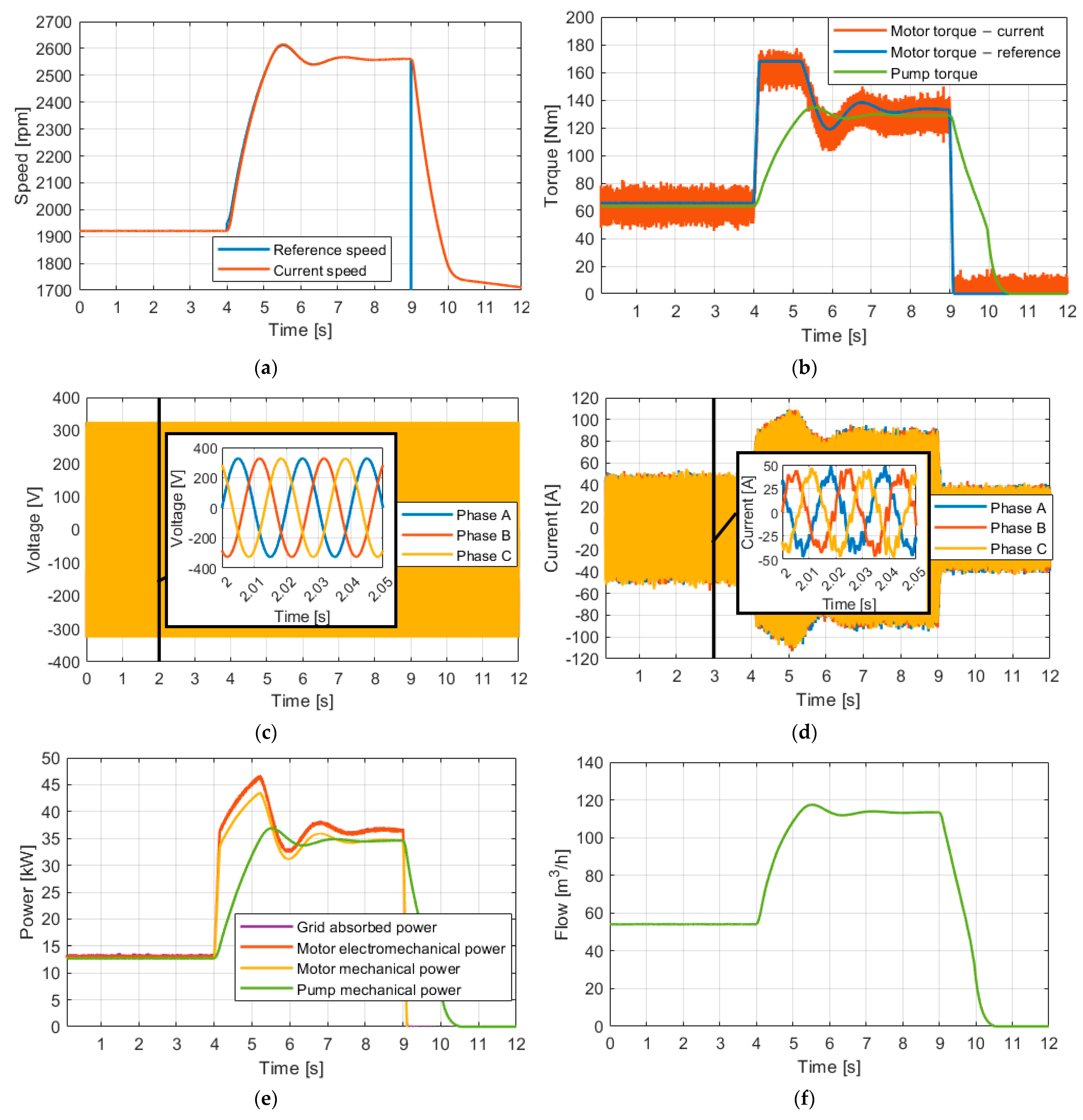
4.2. Response of the Adaptive Control Strategy Operating the Centrifugal Pump at Variable Flow (Pump Discharge)

In the second simulation (12 s), the response of the pumping unit driven by a VFD, operating at variable flow, by a reference flow step from 84 m3/h to 91.5 m3/h, occurring in the fourth second, is presented. In the ninth second, the proposed control strategy stops the pumping system operation.
In Figure 10, it can be seen that the developed strategy for controlling the pump to various flows (discharges) makes the pump flow reach its reference with a small overshoot (MP = 15.2023%) occurring at the peak time Tp = 1.2458 s after the step, with a settling time Ts = 0.4733 s (1% criterium) and a rise time of Tr = 0.138 s (the time for the output to reach from 5% to 95% of the reference).
Figure 11a presents the actual speed of the induction motor and the reference pump flow expressed in the motor’s speed. In the fourth second during the simulation, how the equivalent speed reference changes as the actual volume flow start reaching its reference can be seen.
Figure 11b presents the pump water flow reference expressed in electromechanical torque, the actual electromechanical torque and the load (pump) torque.
Figure 11c shows the three phases of voltage from the power grid being held constant.
In Figure 11d, the current variation of the three phases supplying the induction motor can be seen.
Figure 11e depicts the electrical power absorbed from the power grid, the motor electromechanical power, the mechanical (rotational) power provided by the motor and the pump’s shaft mechanical (rotational) power. During the power transition of the induction motor, the absorbed power from the grid will not exceed the nominal power of the motor. The fluctuations of the absorbed power do not exceed 1% (accepted by most of the power grids).
In Figure 11f, the pump head (pressure) variation during the variable flow (discharge) step response can be seen. According to Figure 11f, it can be seen that during both flow steps from 84 m3/h to 91.5 m3/h in the fourth second and the stop occurring in the ninth second, no over or under pressure occurs that could lead to water hammer or cavitation in the pump [22,24].

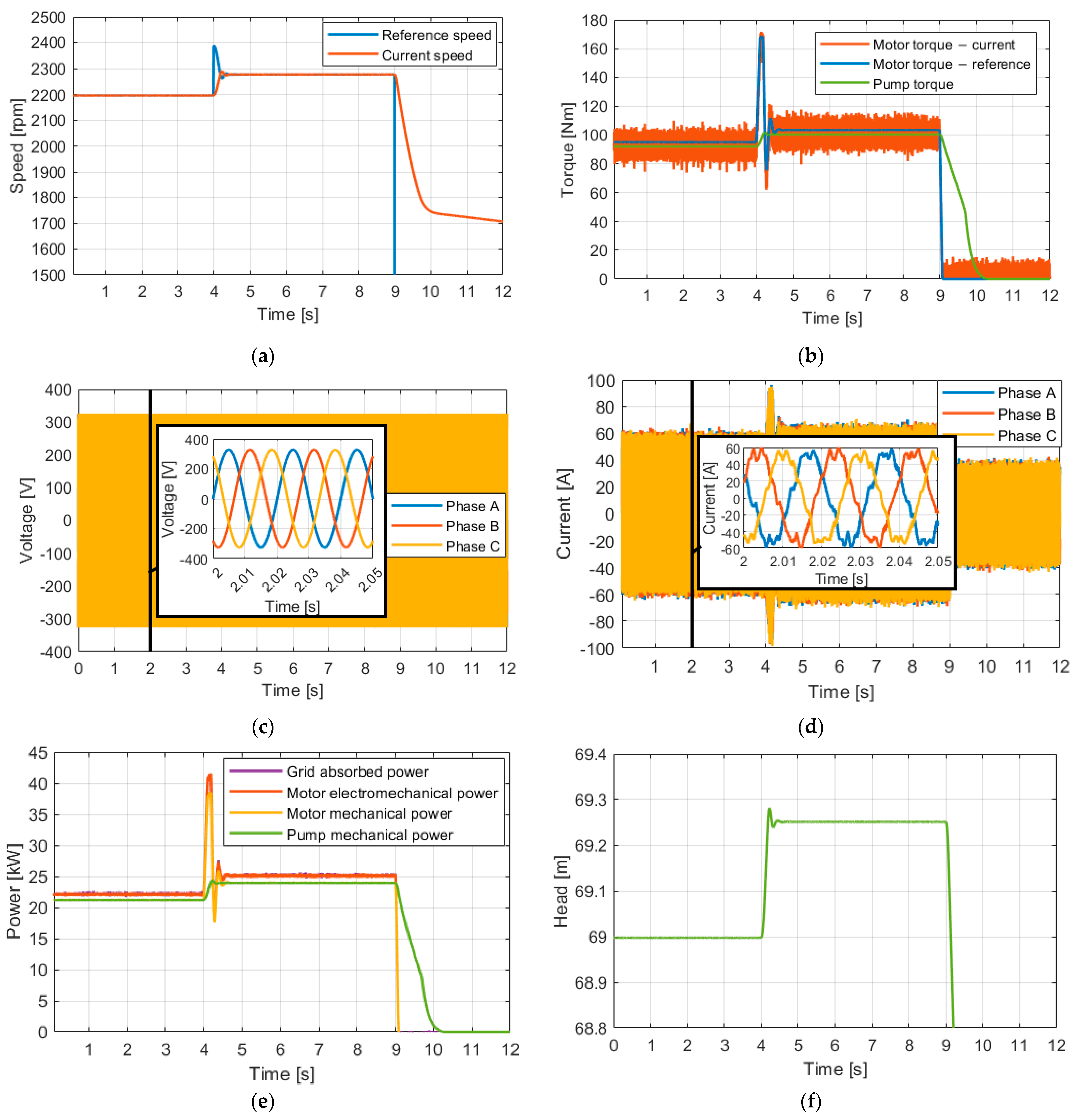
4.3. Response of the Adaptive Control Strategy Operating the Centrifugal Pump at Variable Pressure (Pumping Head)

The third simulation (12 s) presents the response of the pumping unit driven by a VFD in the variable head (pressure) regime, by a reference head step from 68 m to 70 m, occurring in the fourth second. In the ninth second, the proposed control strategy gives the order to stop the pump operation.
In Figure 12, it can be seen that the developed strategy for controlling the pump to various heads (pressures) makes the pump pressure reach its reference with a small overshoot (MP = 7.0261%) occurring at the peak time Tp = 1.5377 s after the step, with a settling time Ts = 2.1090 s (1% criterium) and a rise time of Tr = 1.0084 s (the time for the output to reach from 5% to 95% of the reference).
Figure 13a presents how the actual speed of the induction motor tracks the reference pump head (pressure) expressed in the motor’s speed.
Figure 13b presents the pump head reference expressed in electromechanical torque, the actual electromechanical torque and the load (pump) torque.
Figure 13c shows the three phases of voltage from the power grid being held constant.
In Figure 13d, it can be seen the current variation of the three phases supplying the induction motor during the variable pumping head control strategy.
Figure 13e depicts the electrical power absorbed from the power grid, the motor electromechanical power, the mechanical (rotational) power provided by the motor and the pump’s shaft mechanical (rotational) power. During the power transition of the induction motor, the absorbed power from the grid will not exceed the nominal power of the motor. The fluctuations of the absorbed power do not exceed 1% (accepted by most of the power grids).
In Figure 13f, it can be seen the pump discharge (flow) variation during the variable pumping head control strategy.

4.4. Response Response of the Adaptive Control Strategy Operating the Centrifugal Pump at Variable Available Power (Tracking a Fluctuating and Intermittent Power Source)

The last simulation (9 s) presents the response of the pumping unit driven by a VFD, in the variable power mode, by a reference power step from 22 kW to 25 kW, occurring in the first second. In the sixth second, the proposed control strategy gives the order to stop the pump operation.
Figure 14 depicts the electrical power absorbed from the power grid, the electromechanical motor power, the mechanical (rotational) power provided by the motor and the pump’s shaft mechanical (rotational) power.
Figure 15a presents the actual speed of the induction motor and the reference power expressed in the motor’s speed. The fluctuations of the induction motor’s speed are a maximum of 1.5%.
Figure 15b presents the induction motor power reference expressed in electromechanical torque, the actual electromechanical torque and the pump torque.
Figure 15c shows the three phases of voltage from the power grid being held constant.
In Figure 15d, the current variation of the three phases supplying the induction motor during the variable available power control strategy can be seen.
In Figure 15e, the pump discharge (flow) variation during the variable available power control strategy can be seen.
In Figure 15f, the pressure (pumping head) variation during the variable available power control strategy can be seen. According to Figure 15f, it can be seen that during both the power step from 22 kW to 25 kW occurring in the first second and the stopping order from the sixth second, no over or under pressure occurring that could lead to water hammer or cavitation in the pump [23,24].

5. Conclusions

The current paper proposes a nonlinear mathematical model and an adaptive control strategy for operating PS through a VFD at four different regimes without changing the controller parameters during real-time operation: at variable speed (angular velocity), at variable discharge (pumping flow), at variable pumping head (pressure) and for tracking a variable available power (tracking a fluctuating and intermittent power source such as the power produced by renewable energy conversion systems [1,4]).
The main contribution of the current work, compared to other related work presenting different adaptive control strategies for PS, is that in the current paper, the adaptive character is not ensured by re-tuning the PI controller parameters as in self-tuning controllers [6,7] or by a reference model [8,9] but by readjusting the control law through a change in the control-loop depending on the controlled output of the process (pump speed, pump discharge, pumping head or absorbed power). The deviations of the mentioned controlled outputs from their referenced values are converted into electrical frequency error (the deviation of the current value from its reference), which is the regular input to the already tuned controller; therefore, no controller re-tuning is required.
The personal contribution to the adaptive pumping system control strategy consists of developing several mathematical equations to obtain the pump discharge (flow) error (the deviation of the current value from its reference) (Equation (43)), head (pressure) error (Equation (45)), or absorbed power error (Equation (47)) expressed as a function of electrical frequency error, which is used to develop this control strategy.
The performance of the proposed adaptive control strategy was determined through an in-depth analysis of three performance indicators (overshoot, rise time and settling time) of the pumping system main parameters step responses during four simulations where the pump is driven at variable speed, variable flow, variable pressure and variable power pump. The case studies carried out through simulation led to the conclusion that using the proposed adaptive control strategy ensures good performance. Due to the simplicity and robustness of using only simple PI controllers for managing several operating regimes, the proposed adaptive control strategy is recommended for PS configurations with induction motors driven by VFD with at least one programable PI controller that requires switching during real-time operation between the four different regimes mentioned earlier (without changing the controller parameters on-line).
Finally, as for future work, we propose to experimentally validate the nonlinear mathematical model and adaptive control strategy proposed in the current paper on an existing pumping system powered by a photovoltaic energy conversion system presented in reference [10].

Author Contributions

Conceptualization, D.B. and O.P.; methodology, D.B.; software, D.B.; validation, D.B., O.P., I.F. and C.V.; formal analysis, D.B., O.P., I.F. and C.V.; investigation, D.B., O.P., I.F. and C.V.; resources, D.B., O.P., I.F. and C.V.; data curation, D.B., O.P., I.F. and C.V.; writing—original draft preparation, D.B.; writing—review and editing, D.B., O.P., I.F. and C.V.; visualization, D.B.; supervision, O.P. and I.F.; project administration, D.B.; funding acquisition, I.F. and C.V. All authors have read and agreed to the published version of the manuscript.

Funding

This research was funded by the EEA and Norway Grants under grant No. 2022/337338, entitled Design and Development of an Energy Efficiency Management and Control System with Cost-Effective Solutions for Residential and Educational Buildings.

Data Availability Statement

Not applicable.

Conflicts of Interest

The authors declare no conflict of interest.

Appendix A

Table A1. Variable frequency drive technical specifications [11].
Technical PropertiesVariable Frequency DriveSymbolUnit
ManufacturerNidec Control Techniques--
TypeF300--
Maximum DC voltage980VmaxVFDdcVdc
MMP DC voltage range540–830VVFDdcVdc
AC rated power45PVFDkW
AC rated voltage400VVFDacVac
AC rated frequency50fVFDA
AC maximum continuous current94IVFDA
No-load inverter losses0.0115k0-
Linear inverter losses0.0015k1-
Joule inverter losses0.0438k2-
Table A2. Induction motor technical specifications [17].
Technical PropertiesSubmersible Pump Induction MotorSymbolUnit
ManufacturerCaprari--
TypeMAC625A-8V--
Nominal Power18.5PIM0kW
Nominal Efficiency83%ηIM0%
Nominal Frequency50fIMHz
Nominal Voltage400VIMV
Nominal Current40.2IIMA
Number of poles2Poles-
Rotor synchronous speed3000ωsrpm
Rotor nominal speed2875ω0rpm
Rotor operating speedVariableωrpm
Power factor0.8cos φ-
Table A3. Variable speed centrifugal pump technical specifications [17].
PropertiesValueSymbolUnit
ManufacturerCaprari--
TypeE8P95/7ZC--
Minimum water speed to cool the jacket of the motor0.5 m/s--
Maximum number of starts in one hour20--
Minimum immersion depth507.5 mm--
Pump service flow rate 91.85 m3/hQm3/h
Submersible pump service head 78.12 mHm
Pump rated efficiency 75.63%η%
Pump rated hydraulic power 25.84 kWPhydraulickW
Pump maximum flow rate169.2 m3/hQmaxm3/h
Pump head at theoretical 0 flow rate97.35 mHmaxm
Pump minimum head (at maximum flow rate)83.29 mHminm
Pump efficiency at maximum flow rate81.5%η%
Pump hydraulic power at maximum flow rate30 kWPpumpm3/h
Consumer pressure1.5Hgbar
Well Dynamic head35.7Hgwellmca
Water level variation18.6ΔHgmca
Pipe diameter0.3Dpipem
Head–flow 1st coefficient185.2123Am
Head–flow 2nd coefficient0.2608Bh/m2
Head–flow 3rd coefficient−0.0076Ch/m5
Efficiency-flow 1st coefficient1.8274D1/m2
Efficiency-flow 2nd coefficient−0.104E1/m5

References

  1. Bordeașu, D.; Proștean, O.; Filip, I.; Drăgan, F.; Vașar, C. Modelling, Simulation and Controlling of a Multi-Pump System with Water Storage Powered by a Fluctuating and Intermittent Power Source. Mathematics 2022, 10, 4019. [Google Scholar] [CrossRef]
  2. Al-Khalifah, M.; Mcmillan, G. Control valve versus variable speed drive for flow control. ISA Autom. Week 2012, 60, 42–46. [Google Scholar]
  3. Brogan, A.; Gopalakrishnan, V.; Sturtevant, K.; Valigosky, Z.; Kissock, K. Improving Variable-Speed Pumping Control to Maximize Savings. ASHRAE Trans. 2016, 122, 141–148. [Google Scholar]
  4. Priyadarshi, N.; Ramachandaramurthy, V.K.; Padmanaban, S.K.; Azam, F.; Sharma, A.K.; Kesari, J.P. An ANN Based Intelligent MPPT Control for Wind Water Pumping System. In Proceedings of the 2nd IEEE International Conference on Power Electronics, Intelligent Control and Energy Systems (ICPEICES), Delhi, India, 22–24 October 2018; pp. 443–448. [Google Scholar] [CrossRef]
  5. Sul, S. Control of Electric Machine Drive Systems; John Wiley & Sons: Hoboken, NJ, USA, 2011; pp. 291–294. [Google Scholar]
  6. Mourad, E.; Lachhab, A.; Limouri, M.; Dahhou, B.; Essaid, A. Adaptive control of a water supply system. Control. Eng. Pract. 2001, 9, 343–349. [Google Scholar] [CrossRef]
  7. Kokotovic, V.; Buckman, C. Electric Water Cooling Pump Sensitivity Based Adaptive Control. SAE Int. J. Commer. Veh. 2017, 10, 331–339. [Google Scholar] [CrossRef]
  8. Kiata, E.; Ngasop, N.; Justin, N.S.J.; Djalo, H. Fuzzy Adaptive Control by Reference Model of a Submerged Electric Pump: Application to Photovoltaic Water Pumping. Glob. J. Eng. Sci. 2023, 10, 861–869. [Google Scholar]
  9. Torres, L.H.S.; Schnitman, L.; Felippe de Souza, J.A.M. Model Reference Adaptive Control Applied to the Improvement of the Operational Conditions of a Sucker Rod Pump System. IFAC Proc. Vol. 2010, 43, 231–236. [Google Scholar] [CrossRef] [Green Version]
  10. Bordeașu, D. Study on the implementation of an alternative solution to the current irrigation system. Acta Tech. Napoc. Ser. Appl. Math. Mech. Eng. 2022, 65, 593–602. [Google Scholar]
  11. Nidec. Powerdrive F300; Nidec Control Techniques Ltd.: Newtown, UK, 2017; p. 324. [Google Scholar]
  12. Janevska, G.; Bitola, R.M. Mathematical Modeling of Pump System. Electron. Int. Interdiscip. Conf. 2013, 2, 455–458. [Google Scholar]
  13. Muñoz, J.; Martínez-Moreno, F.; Lorenzo, E. On-site characterisation and energy efficiency of grid-connected PV inverters. Prog. Photovolt. Res. Appl. 2011, 19, 192–201. [Google Scholar] [CrossRef]
  14. Abad, G. Power Electronics and Electric Drives for Traction Applications; John Wiley & Sons, Ltd.: Chichester, UK, 2016. [Google Scholar] [CrossRef]
  15. Abu-Rub, H.; Malinowski, M.; Al-Haddad, K. Power Electronics for Renewable Energy Systems, Transportation and Industrial Applications; John Wiley & Sons Ltd.: Chichester, UK, 2014. [Google Scholar]
  16. Errouha, M.; Motahhir, S.; Combe, Q.; Derouich, A. Intelligent control of induction motor for photovoltaic water pumping system. SN Appl. Sci. 2021, 3, 777. [Google Scholar] [CrossRef]
  17. Caprari, Submersible Electric Pump E8P95/7ZC+MAC870-8V Technical Data Sheet. 2019. Available online: https://ipump.caprarinet.net/ (accessed on 9 October 2021).
  18. Majhi, J.; Nema, S.; Verma, D. Simulation and analysis of solar based water pumping system for hydraulic actuated load. In Proceedings of the 2nd International Conference on Power and Embedded Drive Control (ICPEDC), Chennai, India, 21–23 August 2019. [Google Scholar] [CrossRef]
  19. White, F.M. Fluid Mechanics, 7th ed.; University of Rhode Island: Kingston, RI, USA; McGraw-Hill: New York, NY, USA, 2009. [Google Scholar]
  20. Thorley, A.R.D. Fluid Transients in Pipeline Systems; D. & L. George Ltd Publ.: Herts, UK, 1991. [Google Scholar]
  21. Sabbagh, E.; Sinai, G. A model for optimal real-time computer control of pumping stations in irrigation systems. Comput. Electron. Agric. 1988, 3, 119–133. [Google Scholar] [CrossRef]
  22. Bordeasu, I. Monografia Laboratorului de Cercetare a Eroziunii Prin Cavitatie al Universitatii Polirehnica Timisoara (1960–2020); Editura Politehnica: Timişoara, Romania, 2020. [Google Scholar]
  23. Mitelea, I.; Bordeaşu, I.; Belin, C.; Uţu, I.-D.; Crăciunescu, C.M. Cavitation Resistance, Microstructure, and Surface Topography of Plasma Nitrided Nimonic 80 A Alloy. Materials 2022, 15, 6654. [Google Scholar] [CrossRef] [PubMed]
  24. Bordeasu, I.; Popoviciu, M.O.; Mitelea, I.; Balasoiu, V.; Ghiban, B.; Tucu, D. Chemical and mechanical aspects of the cavitation phenomena. Rev. Chim. 2007, 58, 1300–1304. [Google Scholar]
Figure 1. The layout of the existing industrial high-power pumping system [10].
Machines 11 00688 g001
Figure 2. Diagram of a centrifugal pump driven at variable speed, variable flow, variable pressure and variable available power by an induction motor through a VFD.
Machines 11 00688 g002
Figure 3. Induction Motor dynamic model Simulink diagram.
Machines 11 00688 g003
Figure 4. (a) Pump head-flow H-Q curves at different induction motor frequencies; (b) Pump efficiency-flow η-Q curves at different induction motor frequencies.
Machines 11 00688 g004
Figure 5. (a) Pump Iso-efficiency curve at different induction motor frequencies; (b) Pump Iso-power curve at different induction motor frequencies; (c) Pump Iso-torque curve at different induction motor frequencies; (d) Pump Iso-inertia curve at different induction motor frequencies.
Machines 11 00688 g005
Figure 6. Simulink dynamic model diagram of the centrifugal pump together with the hydraulic network.
Machines 11 00688 g006
Figure 7. VFD control loops block diagram in Simulink.
Machines 11 00688 g007
Figure 8. Response of the induction motor and pump speed (angular velocity) during the operation of the centrifugal pump at variable speed.
Machines 11 00688 g008
Figure 9. Responses during the operation of the centrifugal pump at variable speed (angular velocity): (a) Induction motor and pump torques; (b) Induction motor and pump powers; (c) Voltages of the 3 phases supplying the induction motor; (d) Currents of the 3 phases supplying the induction motor; (e) Pump discharge; (f) Pumping head.
Machines 11 00688 g009
Figure 10. Response of the pump discharge (flow) during the operation of the centrifugal pump at variable pump discharge (flow).
Machines 11 00688 g010
Figure 11. Responses during the operation of the centrifugal pump at variable flow (pump discharge): (a) Induction motor and pump speed; (b) Induction motor and pump torques; (c) Voltages of the 3 phases supplying the induction motor; (d) Currents of the 3 phases supplying the induction motor; (e) Induction motor and pump powers; (f) Pumping head.
Machines 11 00688 g011
Figure 12. Response of the pumping head during the operation of the centrifugal pump at variable pumping head.
Machines 11 00688 g012
Figure 13. Responses during the operation of the centrifugal pump at variable pumping head: (a) Induction motor and pump speed; (b) Induction motor and pump torques; (c) Voltages of the 3 phases supplying the induction motor; (d) Currents of the 3 phases supplying the induction motor; (e) Induction motor and pump powers; (f) Pump discharge.
Machines 11 00688 g013
Figure 14. Response of the induction motor and pump powers during the operation of the centrifugal pump at variable available power.
Machines 11 00688 g014
Figure 15. Responses during the operation of the centrifugal pump at variable available power: (a) Induction motor and pump speed; (b) Induction motor and pump torques; (c) Voltages of the 3 phases supplying the induction motor; (d) Currents of the 3 phases supplying the induction motor; (e) Pump discharge; (f) Pumping head.
Machines 11 00688 g015
Table 1. The 7 operating points of the Variable speed centrifugal pump used in identifying the coefficients of the pump head–flow and efficiency–flow equations.
50 Hz Curve Fitting PointQ [m³/h]H [m]P [kW]η [%]NPSH [m]
10185000
25417736.868.11.8
369.8416641.1976.72.37
485.6815245.11803.22
5101.52133.548.09784.28
6117.3611150.01715.6
7133.28550.0358.357.2
Table 2. Acquisition of nominal data from the sensors during the existing high-power PS operation.
SectorHtotal
(mca)
Q
(m3/h)
Pressure
(bar)
Pressure
Reference (bar)
Power
(kW)
Frequency
(Hz)
168543.48123543.512.02933.0518
276844.188224084.222.31939.0077
37691.54.420837824.425.30140.3471
476904.1683464.224.67640.0732
57285.53.790691913.821.89038.6260
Disclaimer/Publisher’s Note: The statements, opinions and data contained in all publications are solely those of the individual author(s) and contributor(s) and not of MDPI and/or the editor(s). MDPI and/or the editor(s) disclaim responsibility for any injury to people or property resulting from any ideas, methods, instructions or products referred to in the content.

