3.2. Revised Model of Unreformed Cutting Thickness under Tool Wear Conditions
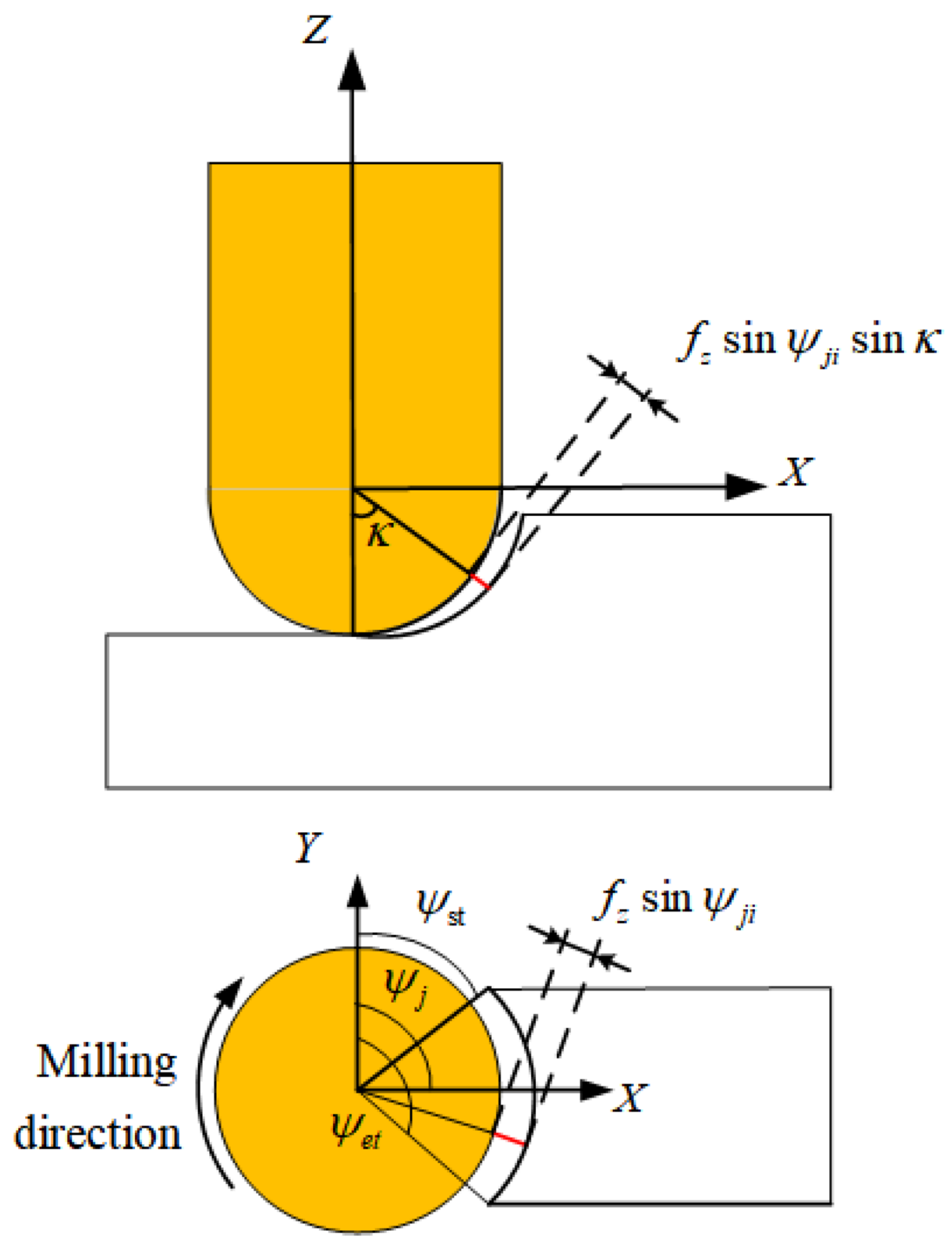
During the ball–end milling cutter section of the cutting process, the cutting edge experiences both rotary motion of the tool and translation movement along the feed direction. A double–bending chip is generated at the apex of the ball–end milling cutter along the cutter helix. This chip–bending phenomenon is closely related to the tool–workpiece cutting contact conditions. The instantaneous undeformed cutting thickness of the ball–end milling cutter is strongly associated with the geometric parameters of the cutter.
As shown in
Figure 5, the instantaneous uncut chip thickness in ball–end milling under the condition of no tool wear [
27] is as follows:
In the formula, represents the cutter’s feed per tooth (mm/z); is the instantaneous radial cutting contact angle (rad) at the spatial position of the I-th cutting element on the J-th cutter tooth; is the axial immersion angle (rad) of the tool and the workpiece.
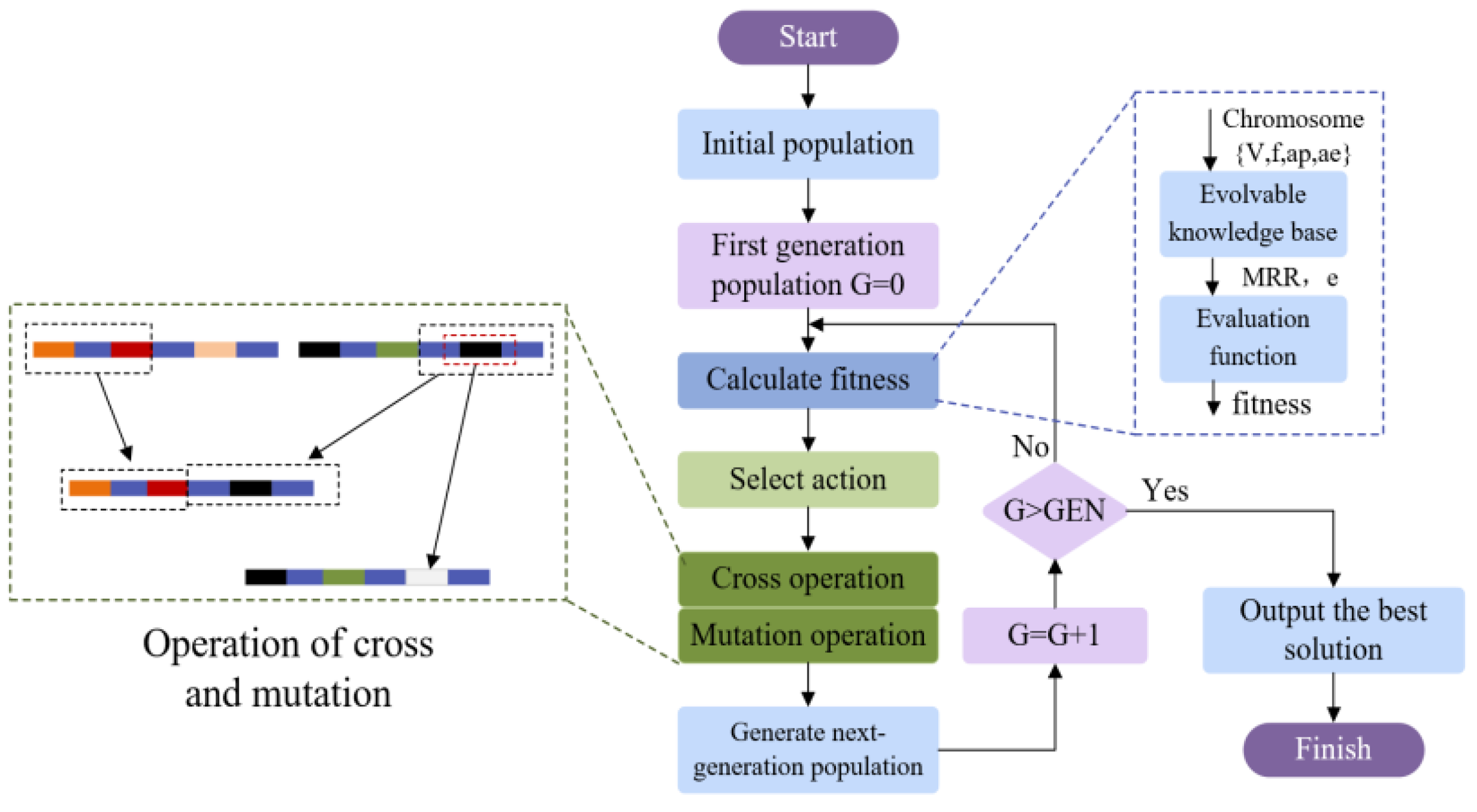
3.2.1. Construction of an Evolutionary Knowledge Base Model Based on Tool Wear Prediction Model
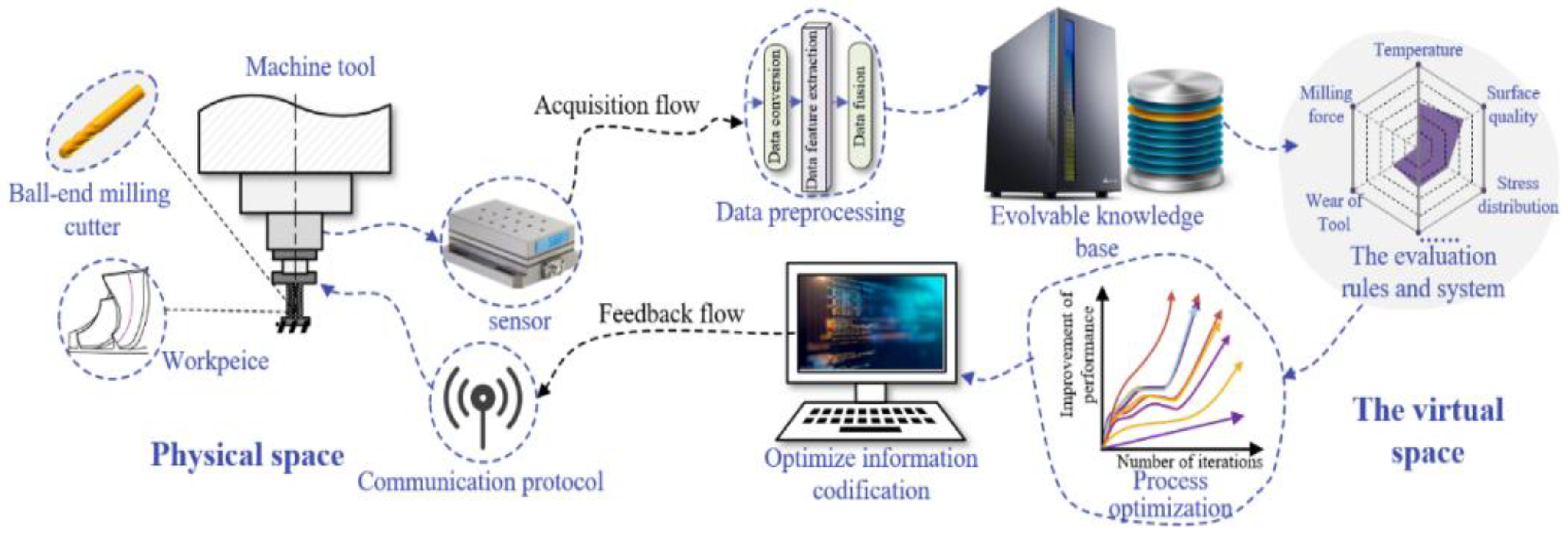
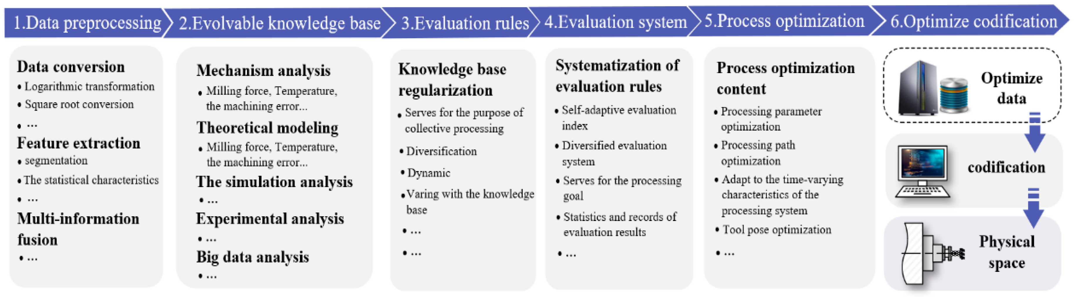
Through the use of machine tool communication protocols, the evolutional knowledge base is capable of reading machining parameters and posture data in real time from the cutting tool, as well as gathering and storing information about the tool’s pose. To expedite the resolution of tool–chip contact areas during the cutting process, the information obtained from the machine tool is compared and extrapolated with the data stored in the evolutionary knowledge base module. In the virtual environment, a model of the unreformed cutting thickness under the condition of tool wear and a model of the tool milling effort in the presence of wear are constructed first. The evolutionary knowledge base is utilized to solve the dynamic cutting force based on rolling data, which is then transmitted to the process evaluation rule module. The resulting process’s overall evaluation data are then relayed to the process optimization module, where the optimization of process parameters is performed.
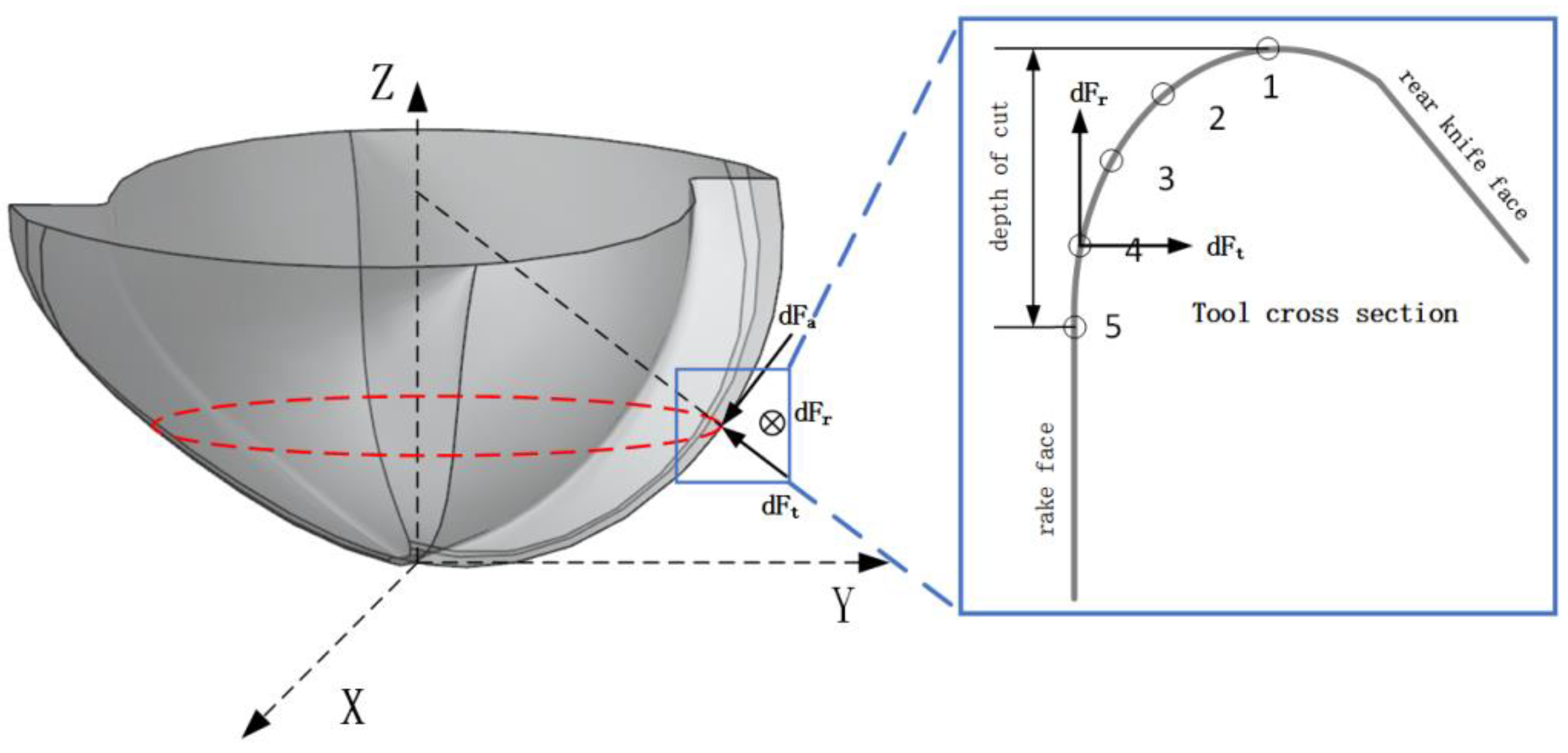
To establish an evolvable knowledge base, the first step is to establish tool wear rules. The cutting force and the hardness of the workpiece and tool can cause friction extrusion, adhesion, diffusion, edge collapse, and plastic deformation, which lead to tool wear and damage. When a tool is worn to a certain extent, it will affect the processing quality and efficiency. A comprehensive analysis of the micro–section of the tool is carried out by cutting the tool section in the XY plane and cutting the surface at the micro–level to approximate it as a turning tool. The force on the selected point is analyzed by taking five evenly spaced points in the intercepting plane for solution. In this article, point 4 is selected as a case for analysis. The cutting force at point 4 can be divided into three parts: the tangential component
along the cutting edge, the radial component
perpendicular to the tool center axis, and the axial component
along the tool axis. The direction of
is along the Z–axis and is not considered in the XY plane, as shown in
Figure 6.
3.2.2. Analysis
Tool metals consist of polycrystalline structures composed of numerous grains of varying shapes. These grains undergo plastic deformation that leads to changes in the lattice arrangement within the metal. The presence of external forces induces shear stress in the material, which causes the lattice to undergo elastic deformation when the stress is small. However, as the stress exceeds a certain threshold, the resistance of the lattice is overcome, causing the grains to slide relative to one another along a crystal plane, a phenomenon referred to as slip. After a certain displacement, the atoms stabilize in a new position, and the slip along the plane ceases due to an increase in resistance. The continued application of shear stress leads to the propagation of slip in other facets of the crystal, resulting in plastic deformation and eventual tool wear.
The formula of the tool wear rule [
28,
29] is as follows:
In the formula, is the wear amount (mm3) and is the empirical wear coefficient (m−1N−1). is the sliding distance (m), is the normal force (N), and is the Vickers hardness number of harder materials.
Where
is the empirical wear coefficient, the calculation formula [
30] is
In the formula, is the cutting speed (m/min), is the sliding distance (m), and is the normal force (N).
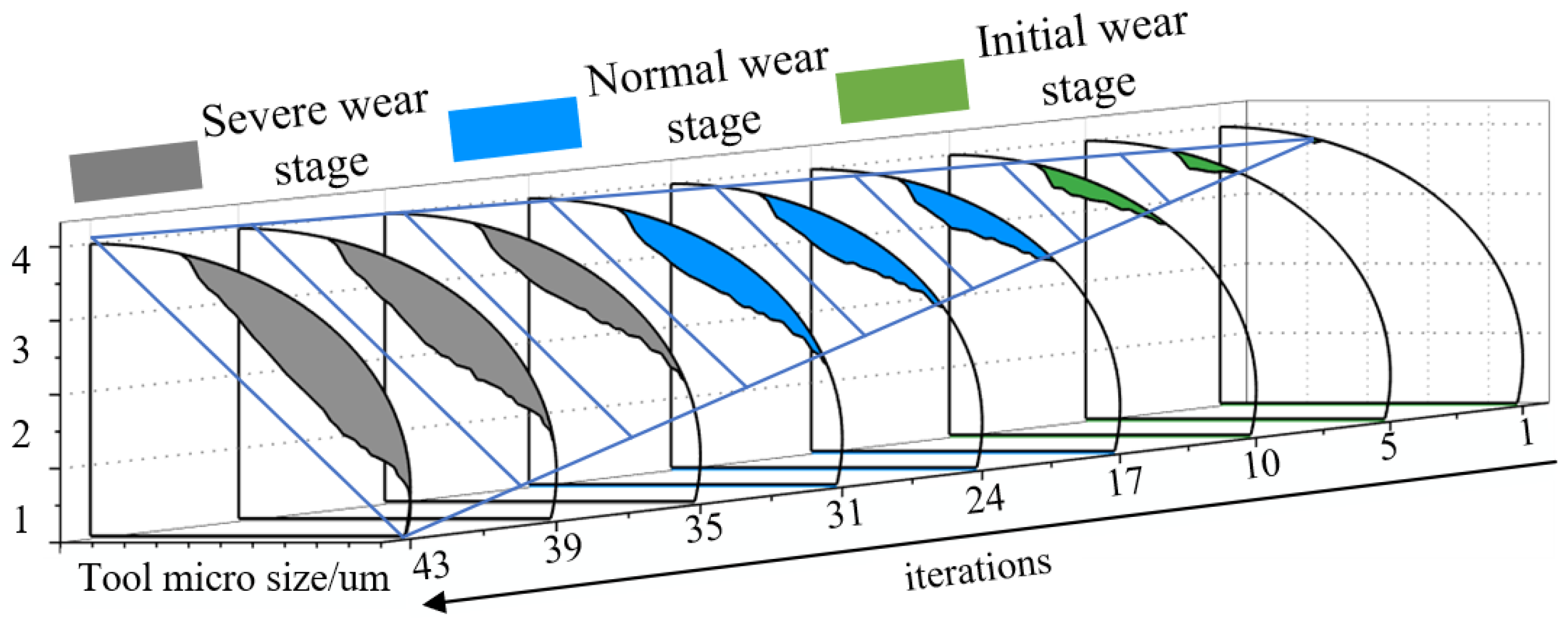
According to the model of tool volume wear, the influence of three stages of tool wear on tool wear was comprehensively considered. The iterative change in the cross–section boundary at point 4 is shown in
Figure 7.
As shown in
Figure 7, point 4 was selected for wear iteration. The different colors in the figure represent different stages of wear and tear. Green represents the initial wear stage of the tool, blue represents the normal wear stage, and gray represents the sharp wear stage. At the bottom right of the picture is the number of iterations. The direction of the arrow in the picture is the increase in the number of iterations. The number corresponds to the change in the tool wear boundary at the selected point 4. The cutting analysis was carried out for other selected points, and the wear boundary in
Figure 8 was obtained after superimposed wear.
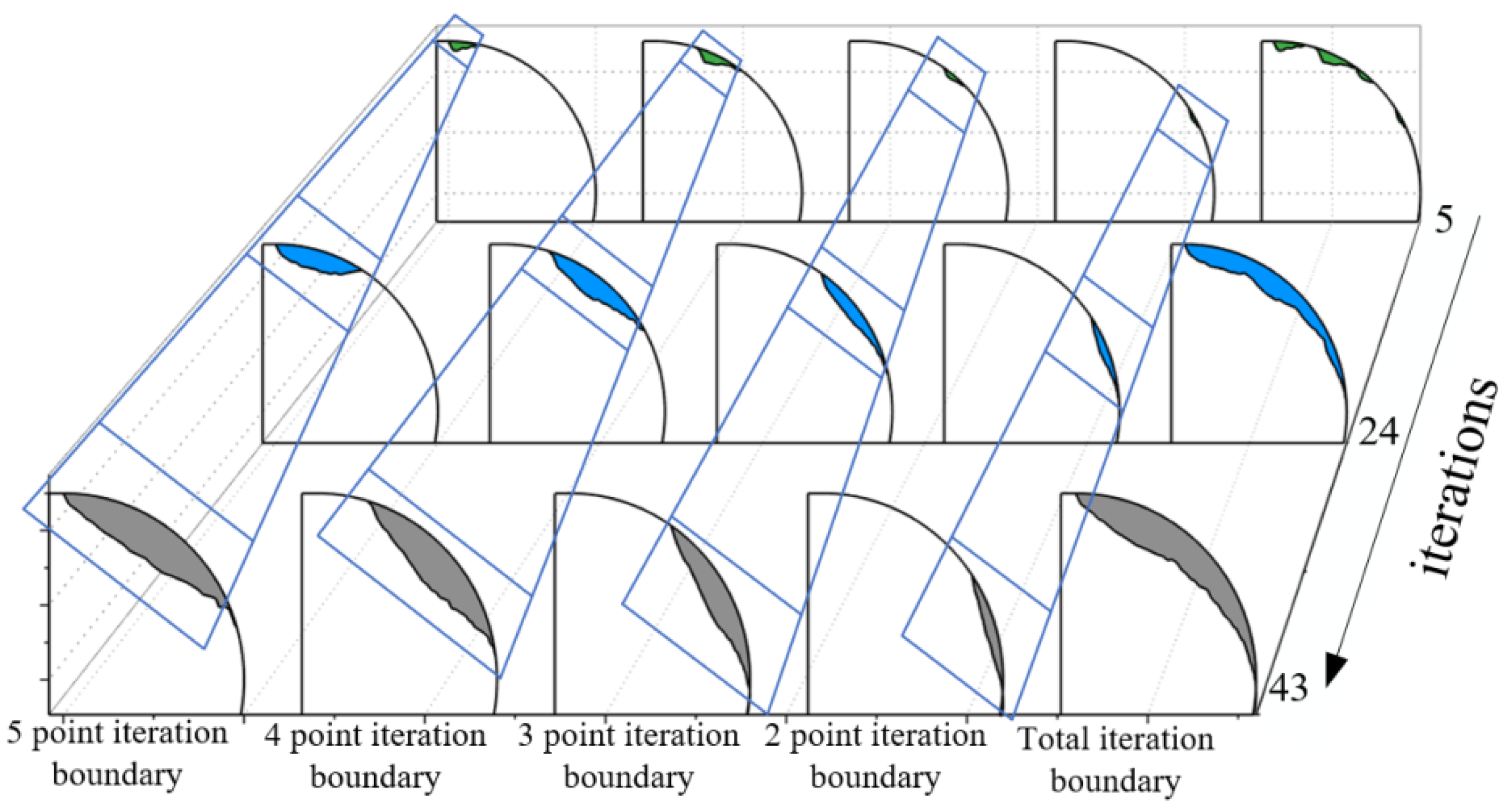
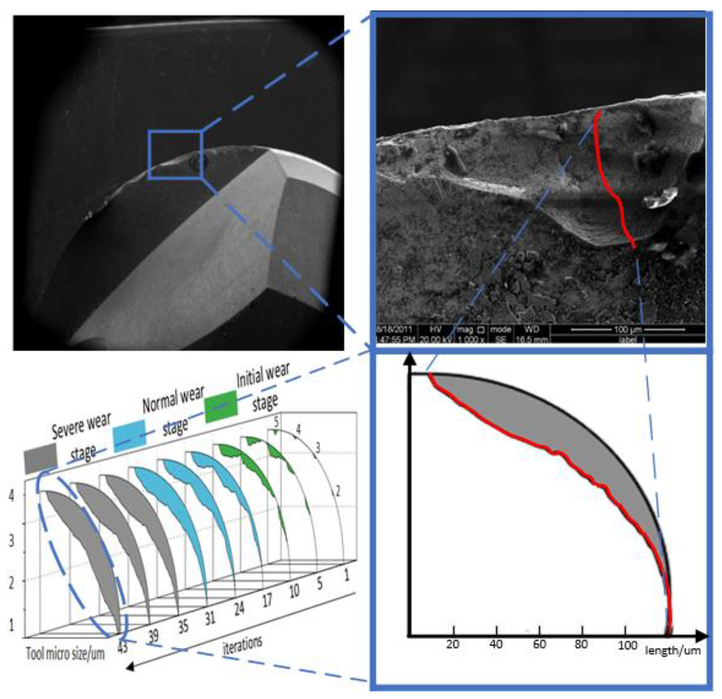
As shown in
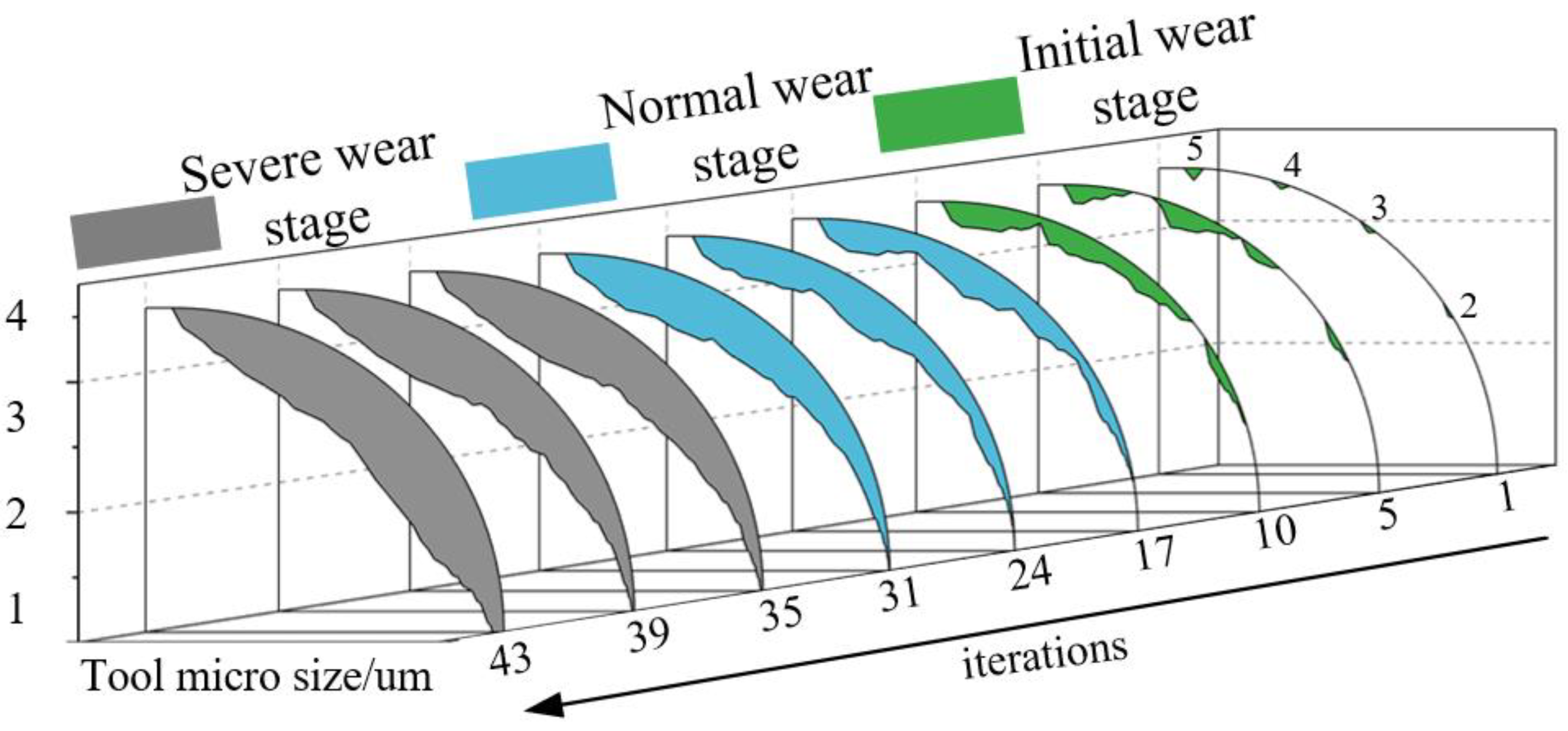
Figure 8, the figure shows the number of iterations on the right, divided into 5, 24, and 43 iterations. The 5 iterations correspond to the initial tool wear stage, the 24 iterations are the normal wear stage, and the 39 iterations are the severe wear stage. Each row corresponding to the number of iterations is the wear boundary of each selected point; the first four graphs of each column are the wear boundaries of points 5, 4, 3, and 2, and the fifth graph is the integrated boundary of the first four points. The first four columns are the changes in the wear boundary for each selected point. The fifth column is the boundary iteration change curve of the overall tool. Considering the influence of the three stages of tool wear on tool wear, the overall change curve of tool section wear is shown in
Figure 8.
As shown in
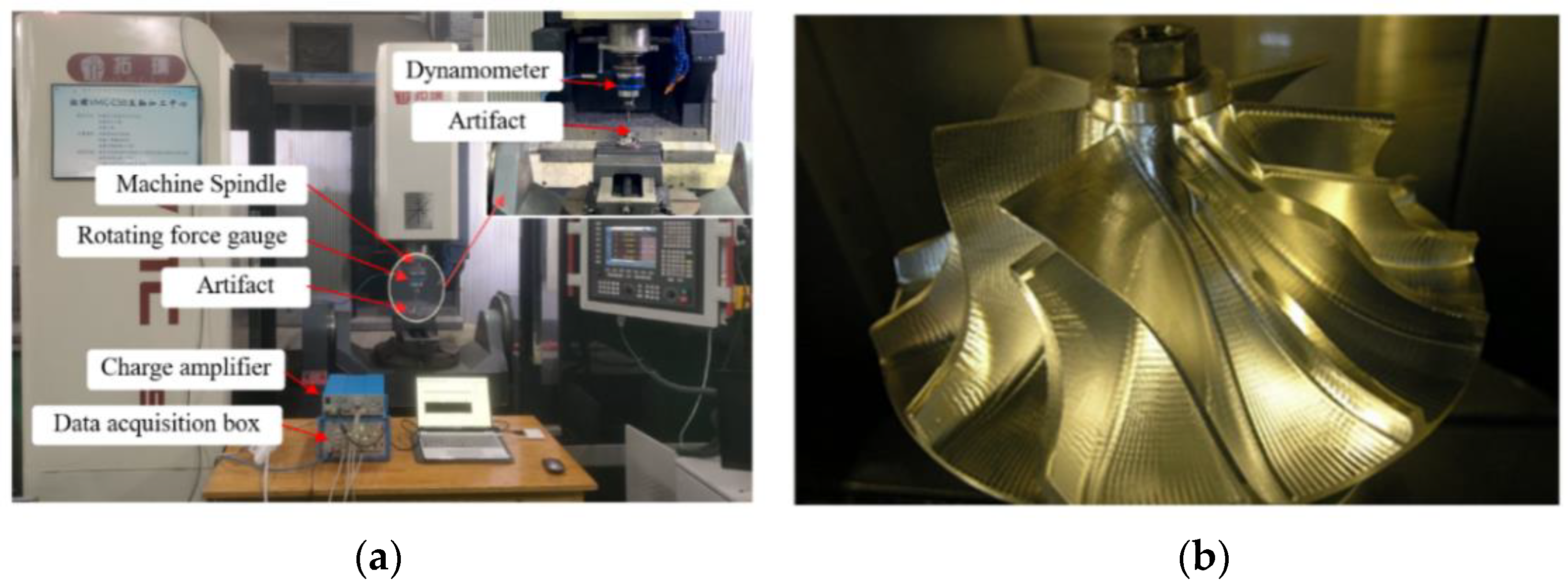
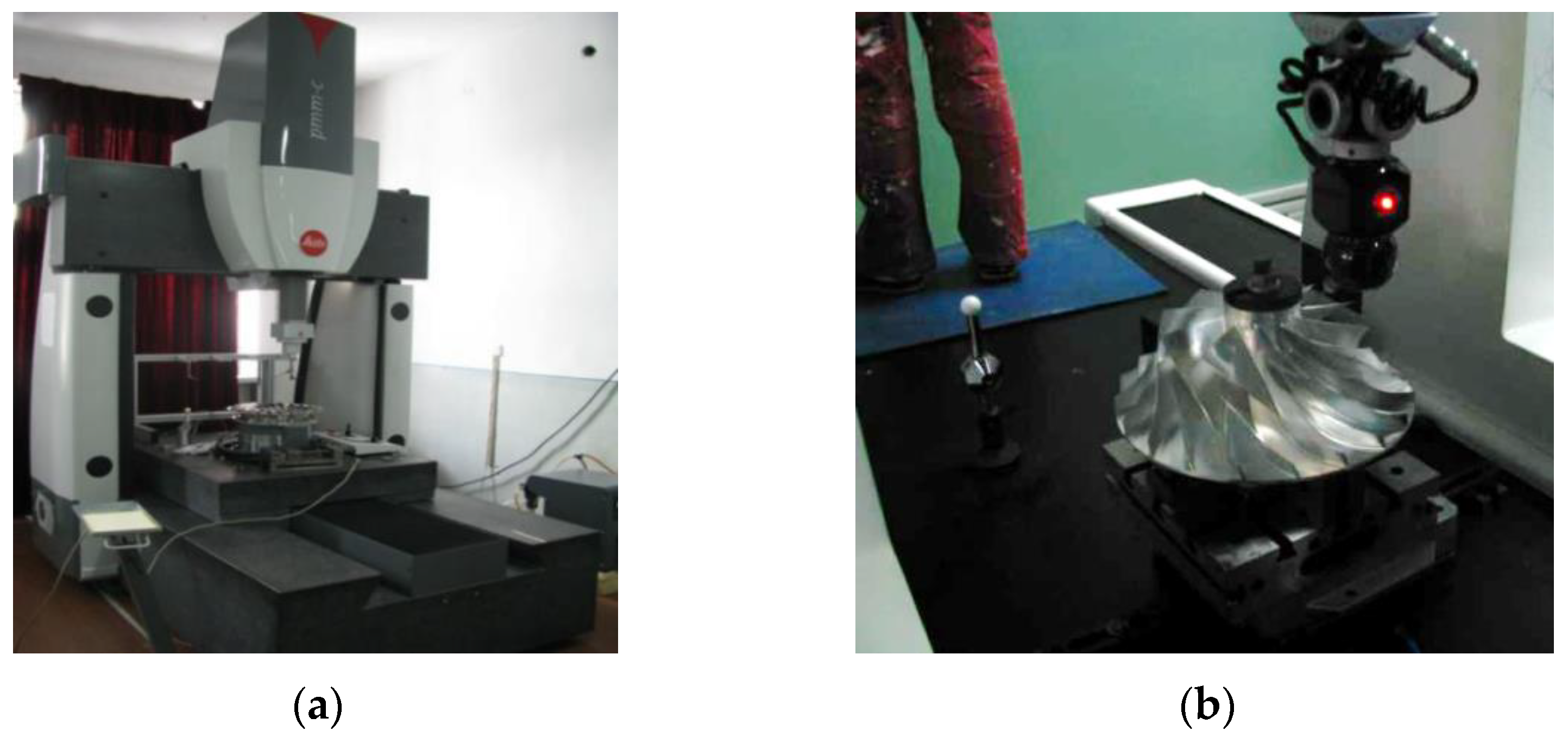
Figure 9, different colors represent different stages of wear. Green is the early wear stage of the tool, blue is the normal wear stage, and gray is the rapid wear stage. The lower right of the figure is the number of iterations, and the direction of the arrow is the increase in the number of tool iterations. Each iteration number corresponds to the overall tool boundary of that iteration. Along with the direction of the arrow is the iterative change in the tool boundary. The tool used is a Dai–Jie double–blade integral carbide ball–end milling cutter, with a diameter of 10 mm, and the material is a hard alloy, as shown
Table 1.
The cutting depth of the tool is 0.2 mm, the rotating speed is 9200 r/min, and the speed
is
When the tool rotates once during cutting, the blade only touches the workpiece at 180°, so the sliding distance
is
In the formula, (min) is the contact time.
According to the calculation, the volume wear rate is about 0.0003 mm
3/min. A microscopic picture of tool wear is shown in
Figure 10.
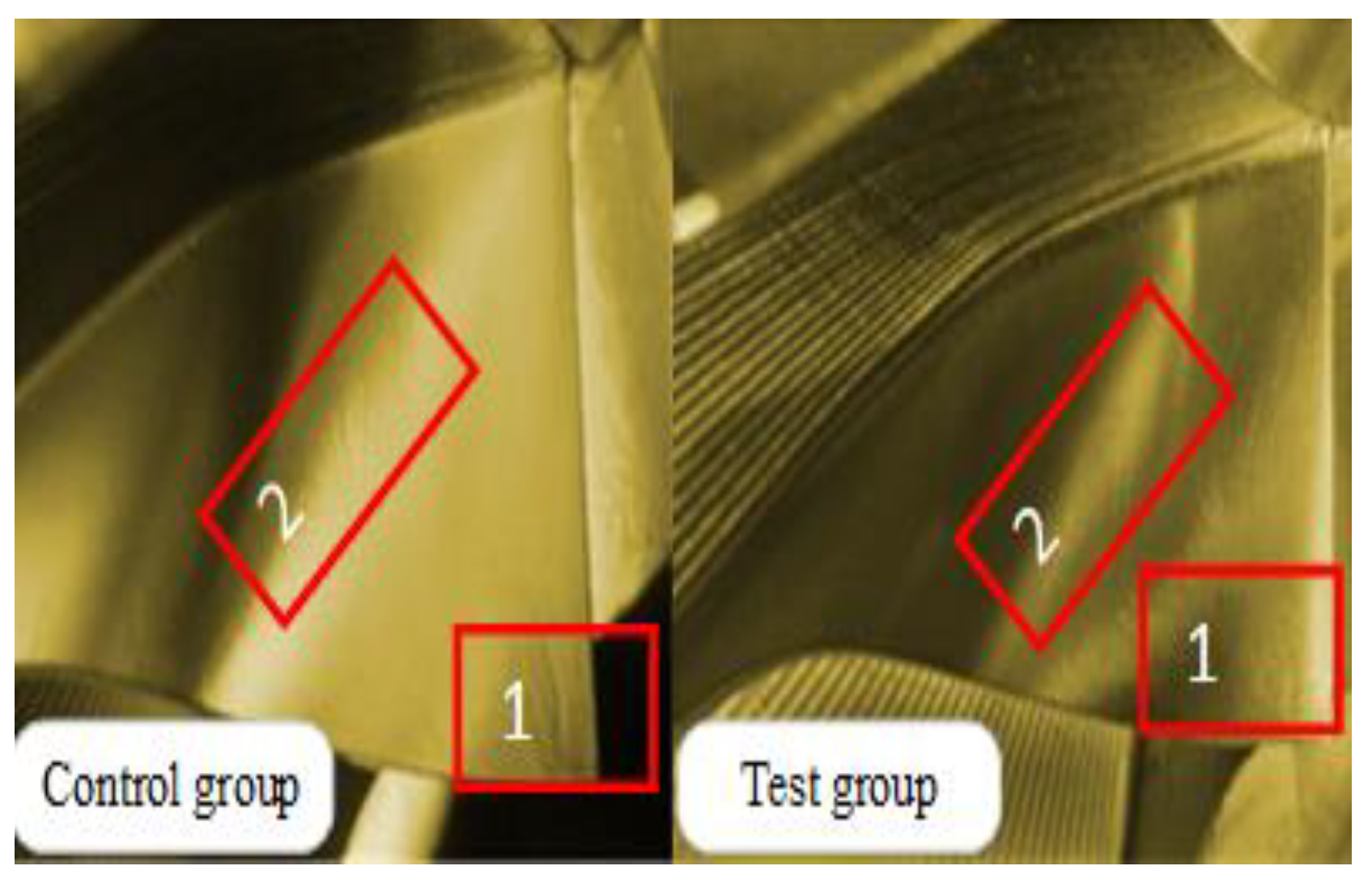
In
Figure 10, the upper half of the figure is the predicted tool wear boundary. The lower part of the figure is the tool wear boundary obtained from the experiment. The red curved boundary is the result of the experimental tool wear boundary and the predicted boundary of the 43rd iteration. There is a certain deviation between the two when compared. The reason for this is that in the method mentioned in this article, the wear volume
is a two–dimensional projection superposed on a certain section of the tool. This method can generate a three–dimensional volume of tool wear by stacking the changes in multi–layer two–dimensional projection, so as to achieve the accurate prediction of tool wear. The model can achieve optimal matching of prediction accuracy and efficiency by adjusting the number of contact points selected on the cross–section. Based on the above research, an evolutionary knowledge base model of the digital–twin tool wear prediction model is established.
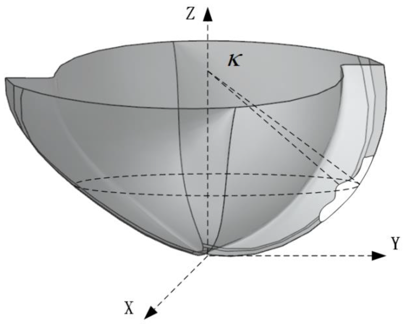
During the cutting process, the tool wear causes the tool’s volume to decrease, leading to changes in the axial immersion angle
of the tool, as illustrated in
Figure 11. The white part of the tool in the figure represents the worn volume of the tool. The reduction in tool volume is evident from the decrease in the axial immersion angle
.
From
Figure 11, it is shown that the axial immersion angle
will decrease with the tool wear, and the change formula of the axial immersion angle
is
In the formula, is the radius. is cutting depth.
The change formula of axial immersion angle
was substituted into the formula of undeformed cutting thickness under the wear condition as follows:
3.3. Milling Force Prediction Model Based on Tool–Chip Contact Relationship
The friction force on the tool flank face is related to the positive pressure and the wear of the flank face. The milling forces solved in this paper include those on the rake face and cutting edge. The partial force of the cutting edge is solved via the micro–element method, and the partial force of the rake face is solved by constructing the stress distribution of the rake face using the tool–chip contact relationship.
When calculating the partial forces on the cutting edge, the cutting edge is micro–elemented, and the force of each cutting edge element is related to the arc length of the element [
31]. The calculation formula is as follows:
In the formula,
,
, and
are, respectively, the tangential force, radial force, and axial force components of the cutting edge element;
is the arc length of the cutting edge element. By integrating the micro–element forces of the cutting edge, the
,
and
components of the milling force received by the cutting edge can be obtained.
,
,
use the milling force coefficient value calculated from the average milling force obtained through experiments proposed by GRADISEK [
32].
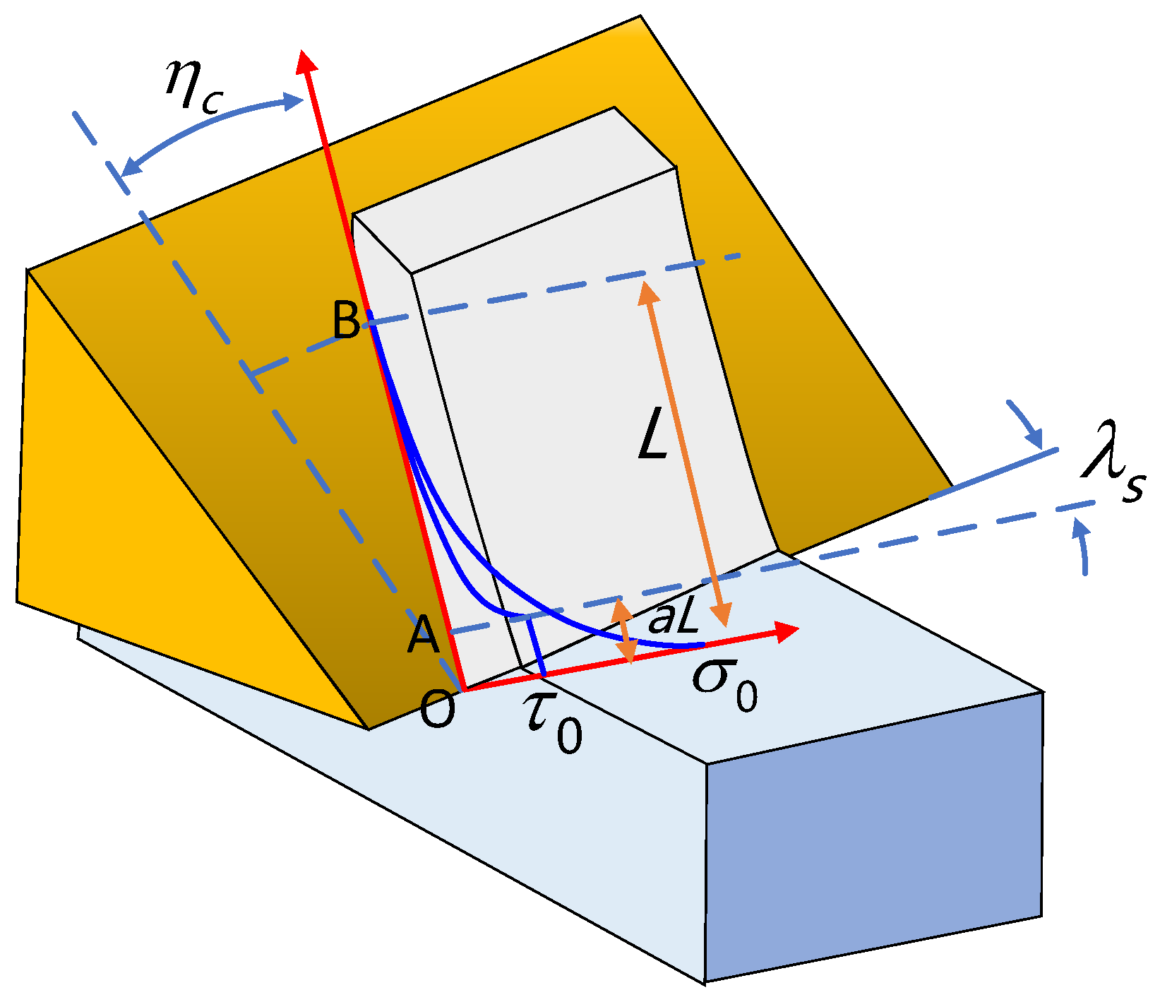
When solving the component forces of the front cutter face, the solution model is the tool–chip contact mechanical model [
33]. The specific situation of the model is shown in
Figure 12.
In
Figure 12,
is the tool tip,
is the bonding area,
is the sliding area, the maximum normal stress at the tool tip is
, the tool–chip contact length is
, and the ratio of the bonding zone length to the tool–chip contact length is
. The friction stress
in the bonding area
is a constant
, and the friction stress in the sliding area is the product of the normal stress and the friction factor. The normal stress
conforms to the power exponential distribution:
is the power exponent, and related experimental studies have shown that the value of b is around 3 [
34]. The maximum stress at the tool tip can be solved using the friction stress
in the bonding area:
In the formula,
is the undeformed chip thickness,
is the cutting outflow angle,
is the shear outflow angle,
is the normal angle of the rake face,
is the shear angle in the normal plane,
is the normal friction angle, and the size of
is close to the shear limit. At this time, the law of friction stress distribution is
In the formula,
is the sliding friction factor, and the size can be calculated from the ball mill test data or through an empirical formula. The scale factor
of the bond zone length to the tool–chip contact length can be solved using the empirical formula:
The integral of normal stress on the rake face is equal to the positive pressure on the rake face, and the integral of friction stress on the rake face is equal to the friction force of the rake face.
In the formula, is the positive pressure on the rake face, and is the friction force on the rake face.
The research object of the tool–chip contact mechanics model for stress distribution and milling force calculation is turning. The milling tool for impeller blade processing is a ball–end milling cutter, and the cutting method is different from turning. When using this model to solve the milling process, the model needs to be revised according to the milling situation. In the solution process, the stress response area is divided into
layers according to parameters such as depth of cut, tool inclination angle, and mesh size. The normal stress and friction force of each layer are as follows:
In the formula, and are the normal stress and friction force of the rake face of the layer, respectively; is the tool–chip contact length extracted from the simulation results of the layer; is the maximum normal stress at the cutting edge of the layer; is the ratio of the layer bonding area to the chip contact area; and is the number of division layers. , , , and other parameters can all be calculated from the tool–chip contact relationship obtained in 4–1.
The direction of the normal stress on the rake face
is perpendicular to the rake facing inward, and the direction of the friction force of
is perpendicular to the normal stress and opposite to the outflow direction of the chips. The normal vector of the rake face can be solved using the equation of the edge line of the ball–end milling cutter and the rake angle of the ball–end milling cutter. The vector equation of the edge line of the ball–end milling cutter can be expressed as
In the formula,
represents the
tooth of the tool,
represents any cutting element on the current tooth,
is the helix angle,
is the helix lag angle,
is the lag angle of the
tooth at this position,
is the radius of the circular section under
, and the vector equation
is the expression in the tool coordinate system.
and
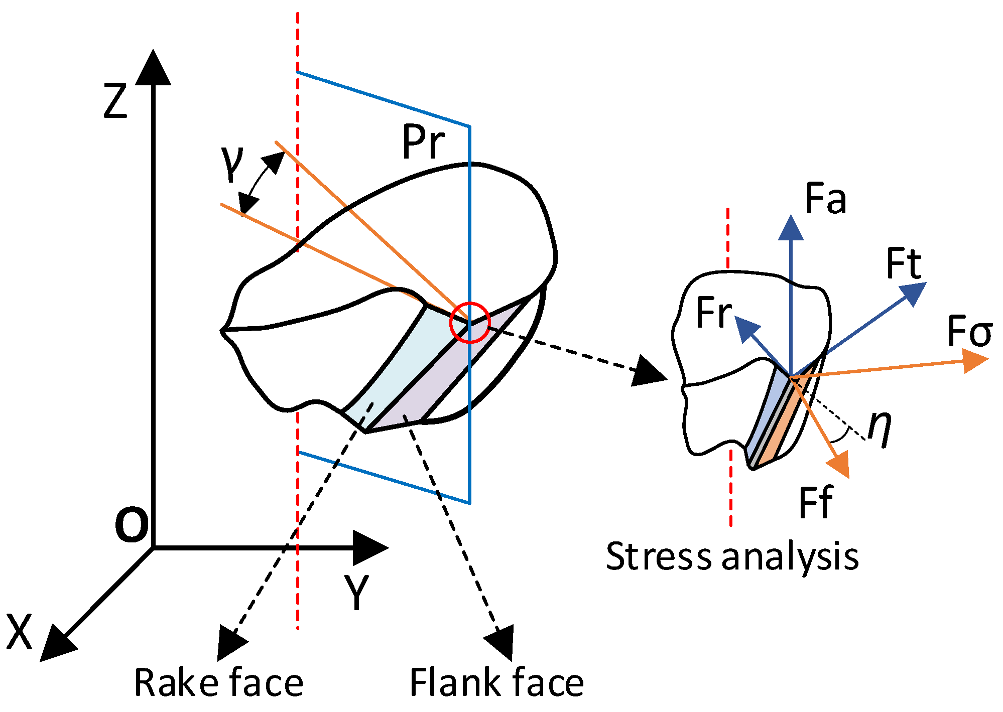
are the unit vectors of each axial direction in the tool coordinate system. The angle and force analysis of the ball–end milling cutter is shown in
Figure 13 below.
In
Figure 13,
is the rake angle of the ball–end milling cutter,
is the chip flow angle, and
is the base plane of the datum reference plane. Assuming that the coordinate of a certain cutting micro–element is
, the relationship between the
milling force coordinate system of the micro–element point and the tool coordinate system is the space translation amount
and angle of rotation around the
axis
. (where
,
). In the
force system coordinate, the normal vector
of the rake face in the coordinate can be obtained through the rake angle
. The edge line equation
of the ball–end milling cutter at this point can be converted into
in the force system coordinate. Then, the normal vector of the rake face can be expressed as
In the formula, is the normal vector of the rake face, which has a vertical relationship with .
The direction vector of the rake face friction force is in the rake face and is opposite to the direction of the cutting flow angle
. Therefore, the friction direction vector can be expressed as
By decomposing the positive pressure and friction of the rake face into the directions of
and then accumulating, the component forces of the force on the rake face in the radial, tangential, and axial directions can be solved:
In the formula, are the axial unit vectors of the force system coordinate. is the normal vector of the rake face of the -th element of the rake face, and is the direction vector of the friction force.
At this time, the milling force of the ball–end milling cutter for processing thin–walled parts is
where
and
refer to the radial, tangential, and axial components of the milling force;
and
refers to the component of milling force experienced by the cutting edge.;
and
are the component of milling force received by the front face;


