Boundary Element Method for Tangential Contact of a Coated Elastic Half-Space

Abstract

We present a formulation of the boundary element method (BEM) for simulating the tangential contact with an elastic half-space coated with an elastic layer with different elastic properties. We use the fast Fourier-transform-based formulation of BEM, while the fundamental solution is determined directly in the Fourier space. Numerical tests are validated by comparison with available asymptotic analytical solutions for a very thin and a very thick layer, as well as with FEM calculations for layers with finite thickness.

1. Introduction

Coatings are widely used to influence and to improve mechanical, electrical, thermal, adhesive, capillary, and other mechanical properties of surfaces; an overview of related problems and applications can be found in [1]. One of the most prominent applications of coatings is wear reduction [2]. The key for understanding and design of coatings is understanding the contact mechanics of coated materials. Other than for the half-space, there are no simple analytical solutions for coated materials. However, analytical solutions have been obtained for limiting cases. Thus, in [3], an analytic asymptotic theory of a normal contact with a thin elastic layer on a rigid foundation was considered. Further developments included analytical work related to rough surfaces [4] as well as contact problems with account of surface tension [5]. Analytical solutions for the tangential contact of coated surfaces has been derived in [6] for isotropic media, in [7] for a transversely isotropic elastic layer, and in [8] for the case of a sliding spherical indenter. Numerical solutions of non-adhesive contact problems for contacts with elastic half-space have been developed since 1990s in the group of Q. Wang (see a review in [9]) and have been extended later to adhesive contacts [10] and contacts with graded materials [11]. Numerical simulation and calculation of normal contact of coated surfaces has also been extensively studied. This includes modelling the contact of specific body shapes [12], or creating contact models, e.g., using finite element analysis [13,14], to investigate different contact configurations. The complete solution for normal contact (both non-adhesive and adhesive) with coated elastic bodies has been given in [15]. Numerical solutions for tangential contact problems of coated surfaces are mostly associated with the study of partial slip, as in [16,17]. In [16], Z. Wang et al. applied a similar procedure to O’Sullivan and King in [8], using Papkovich-Neuber elastic potentials to derive the corresponding frequency response functions. A semi-analytical method (SEM) was used to solve the contact problem. Besides SEM and FEM [18], the BEM is a method that can be used to solve contact problems very efficiently. However, no BEM solution for the tangential contact of coated surfaces has been presented so far. Therefore, an extension of the method developed in [15] to tangential contact is described in the present work; it considers only the tangential part of the contact problem. The FFT-based formulation of the BEM is used for the solution. Since no points inside the body must be discretized, but only the points on the surface, this method has a high numerical efficiency compared to other methods.

The remainder of this paper is structured as follows: Section 2, derives in detail the fundamental solution needed for the BEM formulation. In Section 3, the derived solution is compared with results from the investigation of limiting cases and FEM simulations. In the last section a conclusion is drawn.

2. FFT-Based BEM for Tangential Contact of Coated Surfaces

Consider a coated elastic half-space as schematically shown in Figure 1. The layer having thickness $h$ is assumed to consist of a linearly elastic isotropic material with Young’s modulus $E_1$ and Poisson’s ratio ${\nu }_1$. The half-space is also an isotropic material with elastic constants $E_2$ and ${\nu }_2$. The origin of coordinates is placed on the surface of the layer and the $z$-axis points in the direction of the half-space. The interface between the layer and the underlying elastic half-space has the coordinate $z=h$.

For a numerical simulation, a square area with the side length $L$ is considered, which is discretized with $N$ grid points in each direction. Each square simulation cell has the same size $\Delta x=\Delta y=\Delta$ (see Figure 2). For the application of BEM, it is further assumed that the pressure or stress in each cell is uniform. The usual method for calculating the tangential displacements u resulting from a tangential stress distribution $\mathsf{\tau }$ with the BEM is to perform a direct FFT of the pressure distribution, multiplying it with the FFT of the fundamental solution and finally performing the inverse FFT as follows [15]

$$\mathsf{u}=\mathsf{I}\mathsf{F}\mathsf{F}\mathsf{T}[\mathsf{F}\mathsf{F}\mathsf{T}({\mathsf{U}}_0)\cdot \mathsf{F}\mathsf{F}\mathsf{T}(\mathsf{\tau })],$$

(1)

where ${\mathsf{U}}_0$ is the fundamental solution, giving the displacement of surface points resulting from a single localized tangential force. This procedure is possible for all laterally homogeneous systems, for which the displacement is represented as a convolution of stress distribution and fundamental solution. In Fourier-space the convolution transforms to simple multiplication. A detailed explanation can be found in Ref. [9]. Thus, to calculate the displacements, both the known fundamental solution and the stress distribution must be Fourier-transformed. As suggested in [15], it is much easier to derive the fundamental solution directly in the Fourier-space than in the real space. This also omits one of the operations in (1). In the following, this fundamental solution is to be derived, that is, in terms of Equation (1), the factor $\mathsf{F}\mathsf{F}\mathsf{T}({\mathsf{U}}_0)$.

For the derivation of the fundamental solution in Fourier-space, a distribution of tangential stresses ${\tau }_{xz}$ and ${\tau }_{yz}$ acting on the surface of the layer is considered in the form of a plane wave:

$${\tau }_{xz}={\tau }_x={\tau }_x^0{e}^{i\mathsf{k}\mathsf{r}},$$

(2)

$${\tau }_{yz}={\tau }_y={\tau }_y^0{e}^{i\mathsf{k}\mathsf{r}}.$$

(3)

${\tau }_x^0$ and ${\tau }_y^0$ are here the amplitudes of the corresponding component, $\mathsf{k}$ is the wave vector and $\mathsf{r}$ is the radius vector in the contact plane. In the further text, the symbol $k$, which is not printed in bold, denotes the absolute value of the wave vector, $k=\left|\mathsf{k}\right|$. For simplicity, without loss of generality, we can assume that the direction of the wave vector is given by the $x$-axis. Thus, Equations (2) and (3) can be written as:

$${\tau }_x={\tau }_x^0{e}^{ikx},$$

(4)

$${\tau }_y={\tau }_y^0{e}^{ikx}.$$

(5)

To obtain equations that contain the displacements and can be evaluated using boundary conditions, the equilibrium equation of an elastic isotropic medium is used:

$$\mathrm{grad} \mathrm{div}\hspace{0.17em}\mathsf{u}+(1-2{\nu }_{1,2}){\nabla }^2\mathsf{u}=0,$$

(6)

where $\nabla$ is the (three-dimensional) gradient operator. The displacements $\mathsf{u}$ will in the $x$-direction also have the form of a plane wave:

$$\mathsf{u}=u_x{\mathsf{e}}_{\mathsf{x}}+u_y{\mathsf{e}}_{\mathsf{y}}+u_z{\mathsf{e}}_{\mathsf{z}}=u_x^0(z)e^{ikx}{\mathsf{e}}_x+u_y^0(z)e^{ikx}{\mathsf{e}}_y+u_z^0(z)e^{ikx}{\mathsf{e}}_z.$$

(7)

The vectors ${\mathsf{e}}_x$, ${\mathsf{e}}_y$ and ${\mathsf{e}}_z$ are unit vectors pointing in the direction of the coordinate axes. $u_x$, $u_y$ and $u_z$ denote the projections of the displacement vector on the corresponding directions and the symbols $u_x^0$, $u_y^0$ and $u_z^0$ denote the amplitudes which depend only on the vertical coordinate $z$.

The operators appearing in (6) read:

$$\mathrm{div}\hspace{0.17em}\mathsf{u}=\frac{\partial }{\partial x}\left[u_x^0(z)e^{ikx}\right]+\frac{\partial }{\partial y}\left[u_y^0(z)e^{ikx}\right]+\frac{\partial }{\partial z}\left[u_z^0(z)e^{ikx}\right]=ik{u}_x^0(z)e^{ikx}+\frac{\partial u_z^0(z)}{\partial z}{e}^{ikx},$$

(8)

$$\mathrm{grad} \mathrm{div}\hspace{0.17em}\mathsf{u}=\left[-k^2{u}_x^0(z)e^{ikx}+ik\frac{\partial u_z^0(z)}{\partial z}{e}^{ikx}\right]{\mathsf{e}}_x+\left[ik\frac{\partial u_x^0(z)}{\partial z}{e}^{ikx}+\frac{{\partial }^2{u}_z^0(z)}{\partial z^2}{e}^{ikx}\right]{\mathsf{e}}_z,$$

(9)

$$\begin{array}{l}{\mathbf{\nabla }}^2\mathsf{u}=\\ \left(\frac{{\partial }^2}{\partial x^2}+\frac{{\partial }^2}{\partial z^2}\right)\left[u_x^0(z)e^{ikx}\right]{\mathsf{e}}_x+\left(\frac{{\partial }^2}{\partial x^2}+\frac{{\partial }^2}{\partial z^2}\right)\left[u_y^0(z)e^{ikx}\right]{\mathsf{e}}_y+\left(\frac{{\partial }^2}{\partial x^2}+\frac{{\partial }^2}{\partial z^2}\right)\left[u_z^0(z)e^{ikx}\right]{\mathsf{e}}_z=\\ \\ \left[-k^2{u}_x^0(z)e^{ikx}+\frac{{\partial }^2{u}_x^0(z)}{\partial z^2}{e}^{ikx}\right]{\mathsf{e}}_x+\left[-k^2{u}_y^0(z)e^{ikx}+\frac{{\partial }^2{u}_y^0(z)}{\partial z^2}{e}^{ikx}\right]{\mathsf{e}}_y+\\ \left[-k^2{u}_z^0(z)e^{ikx}+\frac{{\partial }^2{u}_z^0\left(z\right)}{\partial z^2}{e}^{ikx}\right]{\mathsf{e}}_z\hspace{0.17em}\hspace{0.17em}.\end{array}$$

(10)

After substitution of these expressions into (6), we obtain:

$$\frac{{\partial }^2{u}_x^0\left(z\right)}{\partial z^2}+\frac{ik}{1-2{\nu }_{1,2}}\frac{\partial u_z^0\left(z\right)}{\partial z}-\frac{2(1-{\nu }_{1,2})k^2}{1-2{\nu }_{1,2}}{u}_x^0(z)=0,$$

(11)

$$\frac{{\partial }^2{u}_y^0\left(z\right)}{\partial z^2}-k^2{u}_y^0(z)=0,$$

(12)

$$\frac{{\partial }^2{u}_z^0\left(z\right)}{\partial z^2}-\frac{ik}{2({\nu }_{1,2}-1)}\frac{\partial u_x^0(z)}{\partial z}+\frac{(1-2{\nu }_{1,2})k^2}{2({\nu }_{1,2}-1)}{u}_z^0(z)=0.$$

(13)

We look for solutions of the differential equation system in the form:

$$u_x^0\left(z\right)=A{e}^{\lambda z}; u_y^0\left(z\right)=B{e}^{\lambda z};\hspace{0.33em}{u}_z^0\left(z\right)=C{e}^{\lambda z}.$$

(14)

Substituting (14) into Equations (11)–(13), we get:

$$A{\lambda }^2+C\frac{ik}{1-2{\nu }_{1,2}}\lambda -A\frac{2(1-{\nu }_{1,2})k^2}{1-2{\nu }_{1,2}}=0,$$

(15)

$$B{\lambda }^2-B{k}^2=0,$$

(16)

$$C{\lambda }^2-A\frac{ik}{2({\nu }_{1,2}-1)}\lambda +C\frac{(1-2{\nu }_{1,2})k^2}{2({\nu }_{1,2}-1)}=0.$$

(17)

Equation (16) is completely decoupled from (15) and (17) and gives ${\lambda }_{1,2}=k,-k$. Equations (15) and (17) have non-trivial solutions if their determinant vanishes:

$$\left|\begin{array}{cc}{\lambda }^2-\frac{2(1-{\nu }_{1,2})k^2}{1-2{\nu }_{1,2}}& \frac{ik}{1-2{\nu }_{1,2}}\lambda \\ -\frac{ik}{2({\nu }_{1,2}-1)}\lambda & {\lambda }^2+\frac{(1-2{\nu }_{1,2})k^2}{2({\nu }_{1,2}-1)}\end{array}\right|=0.$$

(18)

The solution of this equation gives the characteristic equation with the four roots ${\lambda }_{3,4,5,6}=k,-k,k,-k$. The general solution has the form:

$$u_x^{(1)}(x,z)=u_x^0\left(z\right)e^{ikx}=\left(A_1{e}^{kz}+A_2{e}^{-kz}+A_{3}z{e}^{kz}+A_{4}z{e}^{-kz}\right)e^{ikx},$$

(19)

$$u_y^{(1)}(x,z)=u_y^0\left(z\right)e^{ikx}=\left(B_1{e}^{kz}+B_2{e}^{-kz}\right)e^{ikx},$$

(20)

$$u_z^{(1)}(x,z)=u_z^0\left(z\right)e^{ikx}=\left(C_1{e}^{kz}+C_2{e}^{-kz}+C_{3}z{e}^{kz}+C_{4}z{e}^{-kz}\right)e^{ikx}.$$

(21)

The superscript $\left(1\right)$ indicates that the solutions are valid only inside the coating $(0\le z\le h)$. The general solution inside the half-space has the same form with a different set of coefficients and the superscript $\left(2\right)$:

$$u_x^{(2)}(x,z)=u_x^0\left(z\right)e^{ikx}=\left(A_5{e}^{kz}+A_6{e}^{-kz}+A_{7}z{e}^{kz}+A_{8}z{e}^{-kz}\right)e^{ikx},$$

(22)

$$u_y^{(2)}(x,z)=u_y^0\left(z\right)e^{ikx}=\left(B_3{e}^{kz}+B_4{e}^{-kz}\right)e^{ikx},$$

(23)

$$u_z^{(2)}(x,z)=u_z^0\left(z\right)e^{ikx}=\left(C_5{e}^{kz}+C_6{e}^{-kz}+C_{7}z{e}^{kz}+C_{8}z{e}^{-kz}\right)e^{ikx}.$$

(24)

Substitution of (19)–(21) and (22)–(24) into Equations (11)–(13) leads to:

$$\begin{array}{l}{C}_1=-i\left(A_1-\frac{A_3(3-4{\nu }_1)}{k}\right),\\ C_2=i\left(A_2+\frac{A_4(3-4{\nu }_1)}{k}\right),\\ C_3=-i{A}_3,\hspace{0.33em}{C}_4=i{A}_4\hspace{0.17em}.\end{array}$$

(25)

$$\begin{array}{l}{C}_5=-i\left(A_5-\frac{A_7(3-4{\nu }_2)}{k}\right),\\ C_6=i\left(A_6+\frac{A_8(3-4{\nu }_2)}{k}\right),\\ C_7=-i{A}_7,\hspace{0.33em}{C}_8=i{A}_8\hspace{0.17em}.\end{array}$$

(26)

We use the following boundary conditions:

• The displacements of the half-space in infinite depth are zero:

  $$u_x^{(2)}(x,z\to \infty )=0,\hspace{0.33em}{u}_y^{(2)}(x,z\to \infty )=0,\hspace{0.33em}{u}_z^{(2)}(x,z\to \infty )=0.$$

  (27)
• Continuity of displacements at the interface between the half-space and the coating, as they are assumed to be bonded together:

  $$u_x^{(1)}(x,h)=u_x^{(2)}(x,h),\hspace{0.33em}{u}_y^{(1)}(x,h)=u_y^{(2)}(x,h),\hspace{0.33em}{u}_z^{(1)}(x,h)=u_z^{(2)}(x,h).$$

  (28)
• Continuity of stresses at the interface between the half-space and coating, as they are assumed to be bonded together:

  $${\sigma }_{zz}^{(1)}(x,h)={\sigma }_{zz}^{(2)}(x,h),\hspace{0.33em}{\tau }_{xz}^{(1)}(x,h)={\tau }_{xz}^{(2)}(x,h),\hspace{0.33em}{\tau }_{yz}^{(1)}(x,h)={\tau }_{yz}^{(2)}(x,h).$$

  (29)
• Vanishing of normal stresses at the contact plane:

  $${\sigma }_{zz}^{(1)}(x,z=0)=0.$$

  (30)
• Given x-component of the tangential stress distribution on the surface:

  $${\tau }_{xz}^{(1)}(x,z=0)={\tau }_x={\tau }_x^0{e}^{ikx}.$$

  (31)
• Given y-component of the tangential stress distribution on the surface:

$${\tau }_{yz}^{(1)}(x,z=0)={\tau }_y={\tau }_y^0{e}^{ikx}.$$

(32)

After their evaluation we obtain:

$$A_5=0,\hspace{0.33em}{A}_7=0,\hspace{0.33em}{B}_3=0,\hspace{0.33em}{C}_5=0,\hspace{0.33em}{C}_7=0,$$

(33)

$$A_1{e}^{2hk}+A_2+A_{3}h{e}^{2hk}+A_{4}h-A_6-A_{8}h=0,$$

(34)

$$B_1{e}^{2hk}+B_2-B_4=0,$$

(35)

$$A_{1}k{e}^{2hk}-A_{2}k+A_3{e}^{2hk}(4{\nu }_1+hk-3)+A_4(4{\nu }_1-hk-3)+A_{6}k-A_8(4{\nu }_2-hk-3)=0,$$

(36)

$$\begin{array}{l}\frac{E_1}{1+{\nu }_1}\left[A_{1}k{e}^{2hk}+A_{2}k+A_3{e}^{2hk}\left(2{\nu }_1+hk-2\right)-A_4\left(2{\nu }_1-hk-2\right)\right]-\\ \frac{E_2}{1+{\nu }_2}\left[A_{6}k-A_8\left(2{\nu }_2-hk-2\right)\right]=0\hspace{0.17em}\hspace{0.17em},\end{array}$$

(37)

$$\begin{array}{l}\frac{E_1}{1+{\nu }_1}\left[A_{1}k{e}^{2hk}-A_{2}k+A_3{e}^{2hk}\left(2{\nu }_1+hk-1\right)+A_4\left(2{\nu }_1-hk-1\right)\right]+\\ \frac{E_2}{1+{\nu }_2}\left[A_{6}k-A_8\left(2{\nu }_2-hk-1\right)\right]=0\hspace{0.17em}\hspace{0.17em},\end{array}$$

(38)

$$E_1\left(1+{\nu }_2\right)\left(B_1{e}^{2hk}-B_2\right)+E_2\left(1+{\nu }_1\right)B_4=0,$$

(39)

$$A_{1}k+A_{2}k+2A_3\left(-1+{\nu }_1\right)-2A_4\left(-1+{\nu }_1\right)=0,$$

(40)

$$\frac{E_1}{1+{\nu }_1}\left[A_{1}k-A_{2}k+A_3\left(-1+2{\nu }_1\right)+A_4\left(-1+2{\nu }_1\right)\right]={\tau }_x^0,$$

(41)

$$\frac{E_1}{2\left(1+{\nu }_1\right)}\left[B_{1}k-B_{2}k\right]={\tau }_y^0.$$

(42)

For the plain tangential contact, we search for the displacements in $x$- and $y$- direction at the contact surface $u_x^{(1)}\left(x,z=0\right)$ and $u_y^{(1)}\left(x,z=0\right)$. So, we calculate $A_1,A_2,A_3,A_4$, $B_1$ and $B_2$ using Equations (34)–(42). The solutions for $A_1,A_2,A_3,A_4$ are substituted into (19) and we obtain:

$$u_x^{(1)}\left(x,z=0\right)=\frac{2\left({\nu }_1^2-1\right)\left[A{e}^{-4hk}+4Bhk{e}^{-2hk}+D\right]}{E_{1}k\left[-A{e}^{-4hk}+4B{h}^2{k}^2{e}^{-2hk}+2C{e}^{-2hk}+D\right]}{\tau }_x^0{e}^{ikx}.$$

(43)

Here, the constants $A$, $B$, $C$ and $D$ are given by the following expressions:

$$\begin{array}{l}A=E_2^2{\left(1+{\nu }_1\right)}^2\left(-3+4{\nu }_1\right)+E_1^2{\left(1+{\nu }_2\right)}^2\left(-3+4{\nu }_2\right)-\\ 2E_1{E}_2\left(1+{\nu }_1\right)\left(1+{\nu }_2\right)\left(-3+2{\nu }_1+2{\nu }_2\right)\hspace{0.17em},\end{array}$$

(44)

$$B=E_2^2{\left(1+{\nu }_1\right)}^2+E_1^2{\left(1+{\nu }_2\right)}^2\left(-3+4{\nu }_2\right)-2E_1{E}_2\left(1+{\nu }_1\right)\left(-1+{\nu }_2+2{\nu }_2^2\right),$$

(45)

$$\begin{array}{l}C=E_2^2{\left(1+{\nu }_1\right)}^2\left(5-12{\nu }_1+8{\nu }_1^2\right)+E_1^2{\left(1+{\nu }_2\right)}^2\left(-3+4{\nu }_2\right)-\\ 2E_1{E}_2\left(-1+{\nu }_1+2{\nu }_1^2\right)\left(-1+{\nu }_2+2{\nu }_2^2\right)\hspace{0.17em},\end{array}$$

(46)

$$\begin{array}{l}D=-E_2^2{\left(1+{\nu }_1\right)}^2\left(-3+4{\nu }_1\right)-E_1^2{\left(1+{\nu }_2\right)}^2\left(-3+4{\nu }_2\right)+\\ 2E_1{E}_2\left(1+{\nu }_1\right)\left(1+{\nu }_2\right)\left(5-6{\nu }_2+{\nu }_1\left(-6+8{\nu }_2\right)\right)\hspace{0.17em}\hspace{0.17em}.\end{array}$$

(47)

Now we substitute $B_1$ and $B_2$ into (20) and obtain:

$$u_y^{(1)}\left(x,z=0\right)=\frac{2\left(1+{\nu }_1\right)\left[F{e}^{-2hk}-G\right]}{E_{1}k\left[F{e}^{-2hk}+G\right]}{\tau }_y^0{e}^{ikx},$$

(48)

where the constants $F$ and $G$ are given by the following expressions:

$$F=E_2\left(1+{\nu }_1\right)-E_1\left(1+{\nu }_2\right),$$

(49)

$$G=E_2\left(1+{\nu }_1\right)+E_1\left(1+{\nu }_2\right).$$

(50)

We write the solutions (43) and (48) for $u_x$ and $u_y$ in the following abbreviated form:

$$\begin{array}{l}{u}_x=u_x^{(1)}\left(x,z=0\right)={\mathsf{\Phi }}_x\left(k\right){\tau }_x^0{e}^{ikx}\hspace{0.17em},\\ u_y=u_y^{(1)}\left(x,z=0\right)={\mathsf{\Phi }}_y\left(k\right){\tau }_y^0{e}^{ikx}\hspace{0.17em}.\end{array}$$

(51)

In the above derivation, we have chosen the $x$-axis along the wave vector. However, on the back Fourier transformation, integration goes over all possible wave vectors at the given stress on the surface. To be able to perform this operation, we now write the result (51) in a coordinate system where both the wave vector and the stress vector have arbitrary directions. To this end a new coordinate system $\left(x^{\prime },y^{\prime }\right)$ is considered, which is rotated relative to $\left(x,y\right)$ by angle $\phi$ as shown in Figure 3.

The coordinate transformations read:

$$\begin{array}{l}{u}_{x^{\prime }}=u_x\cos \phi -u_y\sin \phi \hspace{0.17em},\\ u_{y^{\prime }}=u_x\sin \phi +u_y\cos \phi \hspace{0.17em},\end{array}$$

(52)

$$\begin{array}{l}{\tau }_x^0={\tau }_{x^{\prime }}^0\cos \phi +{\tau }_{y^{\prime }}^0\sin \phi \hspace{0.17em},\\ {\tau }_y^0=-{\tau }_{x^{\prime }}^0\sin \phi +{\tau }_{y^{\prime }}^0\cos \phi \hspace{0.17em},\end{array}$$

(53)

$$\begin{array}{l}x=x^{\prime }\cos \phi +y^{\prime }\sin \phi \hspace{0.17em},\\ y=-x^{\prime }\sin \phi +y^{\prime }\cos \phi \hspace{0.17em}.\end{array}$$

(54)

Substitution of (53) and (54) into (51) gives:

$$\begin{array}{l}{u}_x={\mathsf{\Phi }}_x\left(k\right)\left({\tau }_{x^{\prime }}^0\cos \phi +{\tau }_{y^{\prime }}^0\sin \phi \right)e^{ik\left(x^{\prime }\cos \phi +y^{\prime }\sin \phi \right)}\hspace{0.17em},\\ u_y={\mathsf{\Phi }}_y\left(k\right)\left(-{\tau }_{x^{\prime }}^0\sin \phi +{\tau }_{y^{\prime }}^0\cos \phi \right)e^{ik\left(x^{\prime }\cos \phi +y^{\prime }\sin \phi \right)}\hspace{0.17em}.\end{array}$$

(55)

Further substitution of (55) into (52) leads to the result:

$$\begin{array}{l}{u}_{x^{\prime }}=\left[{\mathsf{\Phi }}_x\left(k\right)\left({\tau }_{x^{\prime }}^0{\cos }^2\phi +{\tau }_{y^{\prime }}^0\sin \phi \cos \phi \right)-{\mathsf{\Phi }}_y\left(k\right)\left(-{\tau }_{x^{\prime }}^0{\sin }^2\phi +{\tau }_{y^{\prime }}^0\sin \phi \cos \phi \right)\right]e^{ik\left(x^{\prime }\cos \phi +y^{\prime }\sin \phi \right)}\hspace{0.17em},\\ u_{y^{\prime }}=\left[{\mathsf{\Phi }}_x\left(k\right)\left({\tau }_{x^{\prime }}^0\sin \phi \cos \phi +{\tau }_{y^{\prime }}^0{\sin }^2\phi \right)+{\mathsf{\Phi }}_y\left(k\right)\left(-{\tau }_{x^{\prime }}^0\sin \phi \cos \phi +{\tau }_{y^{\prime }}^0{\cos }^2\phi \right)\right]e^{ik\left(x^{\prime }\cos \phi +y^{\prime }\sin \phi \right)}\hspace{0.17em}.\end{array}$$

(56)

If we assume that the stress vector $\mathsf{\tau }$ is directed along the axis $x^{\prime }$, then ${\tau }_{y^{\prime }}^0=0$ and (56) takes the form:

$$\begin{array}{l}{u}_{x^{\prime }}={\tau }_{x^{\prime }}^0\left[{\mathsf{\Phi }}_x\left(k\right){\cos }^2\phi +{\mathsf{\Phi }}_y\left(k\right){\sin }^2\phi \right]e^{ik\left(x^{\prime }\cos \phi +y^{\prime }\sin \phi \right)}\hspace{0.17em},\\ u_{y^{\prime }}={\tau }_{x^{\prime }}^0\left[{\mathsf{\Phi }}_x\left(k\right)-{\mathsf{\Phi }}_y\left(k\right)\right]\sin \phi \cos \phi e^{ik\left(x^{\prime }\cos \phi +y^{\prime }\sin \phi \right)}\hspace{0.17em}.\end{array}$$

(57)

These equations show that the traction along the axis $x^{\prime }$ lead to displacements both in the direction of traction and perpendicular to it. The reverse is also true: a displacement in the direction $x^{\prime }$ will lead to the appearance of stress component perpendicular to this direction.

Now it is possible to calculate the displacements in the direction of the loading and perpendicular to it. To use it in a BEM code, we need to convert it into an inverse Fast Fourier Transform so that:

$$u_x=\mathsf{I}\mathsf{F}\mathsf{F}\mathsf{T}\left[\left\{{\mathsf{\Phi }}_x\left(k\right){\cos }^2\phi +{\mathsf{\Phi }}_y\left(k\right){\sin }^2\phi \right\}\hspace{0.33em}\cdot \hspace{0.33em}\mathsf{F}\mathsf{F}\mathsf{T}\left(\mathsf{\tau }\right)\right]\hspace{0.17em},$$

(58)

$$u_y=\mathsf{I}\mathsf{F}\mathsf{F}\mathsf{T}\left[\left\{\left[{\mathsf{\Phi }}_x\left(k\right)-{\mathsf{\Phi }}_y\left(k\right)\right]\sin \phi \cos \phi \right\}\hspace{0.33em}\cdot \hspace{0.33em}\mathsf{F}\mathsf{F}\mathsf{T}\left(\mathsf{\tau }\right)\right]\hspace{0.17em}.$$

(59)

The operation $〈\cdot 〉$ denotes an element-wise multiplication since both terms are 2D matrices. For the inverse problem, the calculation of the tangential stress distribution from a given displacement field, the conjugate gradient method can be used. This completes the formulation of the BEM for the purely tangential contact of coated systems.

3. Comparison with Limiting Cases and FEM Solutions

In order to check the correctness of the derivation and the resulting Equations (58) and (59), comparisons are made with other solutions. For this purpose, limiting cases are investigated and results from FEM calculations are used. The limiting cases are, first, the case of a layer with infinite thickness and, second, the case of a thin layer on a rigid surface. Comparison solutions can be easily created for these two cases.

To start with the general case, the comparison with FEM solutions is presented first. More detailed information on the FEM model and how to obtain the FEM results can be found in Appendix A. For comparison, we consider a boundary value problem in which a circular contact area of diameter $2a$ is displaced tangentially by $u_x$. The resulting tangential force $F_x$ and the resulting tangential contact stiffness $k_T$ are calculated. We are interested in the influence of the ratio of elastic moduli $E_1/E_2$ on the contact stiffness at different ratios $a/h$. The Poisson’s ratio of the layer and the substrate should be the same $\left({\nu }_1={\nu }_2=0.3\right)$. To work only with dimensionless parameters, the normalized tangential contact stiffness $k_{T,\mathrm{n}\mathrm{o}\mathrm{r}\mathrm{m}}$ is defined, which can be calculated as follows:

$$k_{T,\mathrm{n}\mathrm{o}\mathrm{r}\mathrm{m}}=\frac{k_T}{k_{T,\mathrm{h}\mathrm{o}\mathrm{m}}}.$$

(60)

The contact stiffness resulting from BEM or FEM simulations is thus divided by the contact stiffness that would result without the layer. This contact stiffness can be calculated analytically for our case [19]

$$k_{T,\mathrm{hom}}=2a{G}_2^{*}\hspace{0.17em},$$

(61)

with $G_2^{*}=4G_2/\left(2-{\nu }_2\right)$ and $G_2$ as the shear modulus of the substrate.

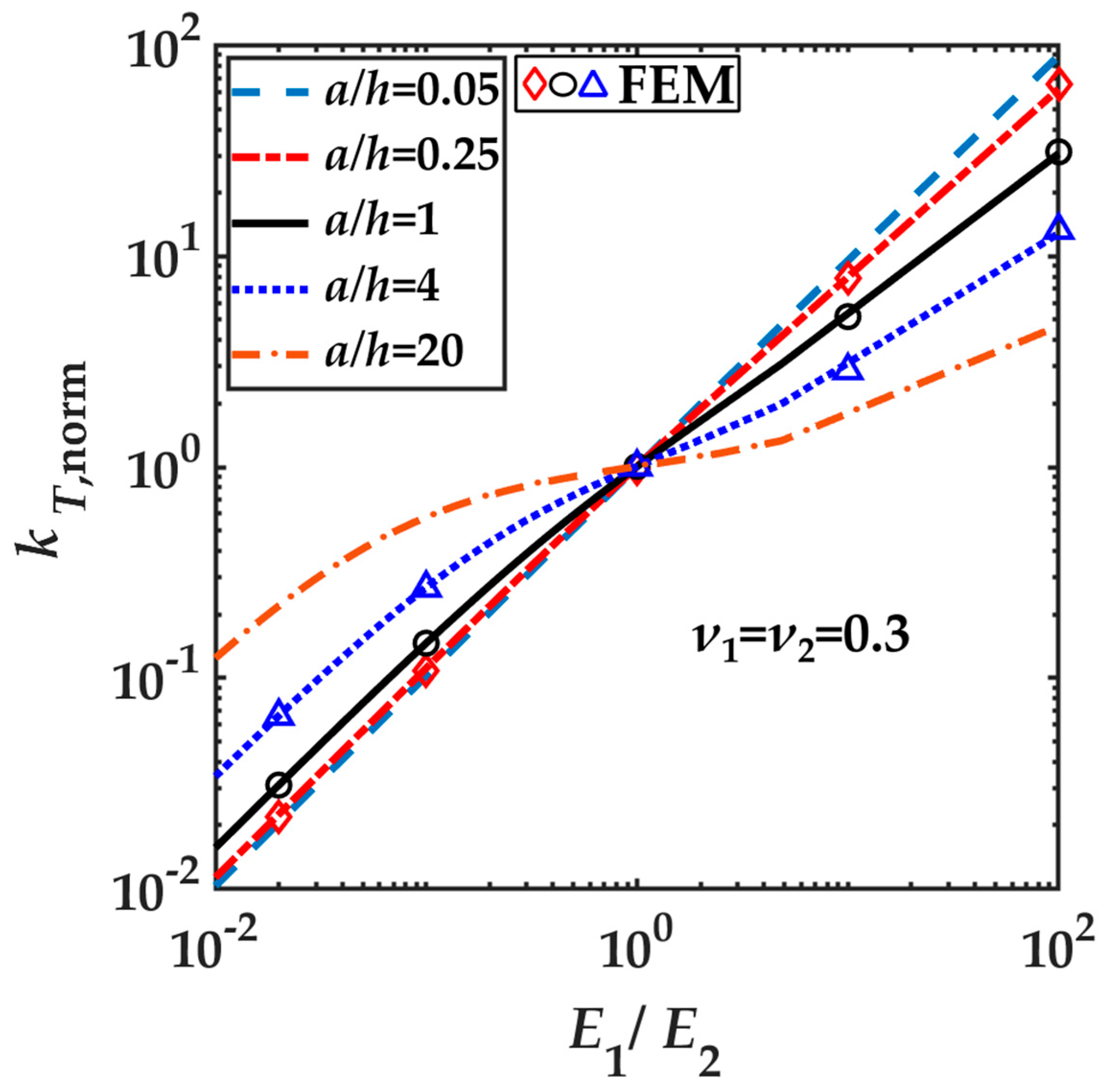
Figure 4 shows the results and the comparison. The normalized tangential contact stiffness is plotted against the ratio of elastic moduli for different ratios $a/h$. The different types of lines represent the BEM solutions, and the markings represent the FEM solutions. The comparison was made for each case: the contact radius is smaller, larger, or equal to the layer thickness. In addition, two other ratios $a/h$ were calculated with the BEM.

As can be seen, the agreement between the results of the two simulation methods is very good. Moreover, all curves meet at the point $k_{T,\mathrm{n}\mathrm{o}\mathrm{r}\mathrm{m}}=1$ and $E_1/E_2=1$, as it is to be expected, since it is the case of the homogeneous half-space. We can also see that the layer stiffness has a direct influence on the tangential contact stiffness of the contact system. When $E_1>E_2$, $k_{T,\mathrm{n}\mathrm{o}\mathrm{r}\mathrm{m}}>1$, since the contact stiffness is larger than in the homogeneous case. The reverse case also applies, so that $k_{T,\mathrm{n}\mathrm{o}\mathrm{r}\mathrm{m}}<1$ if $E_1<E_2$. The influence of the layer depends of course on its thickness. For thinner layers $\left(a/h>1\right)$, $k_{T,\mathrm{n}\mathrm{o}\mathrm{r}\mathrm{m}}$ tends to become a constant with a value of $1$, since the properties of the substrate dominate the contact configuration. For thicker layers $\left(a/h<1\right)$, the relation between $k_{T,\mathrm{n}\mathrm{o}\mathrm{r}\mathrm{m}}$ and the ratio $E_1/E_2$ becomes linear, as the properties of the layer are more dominant, which can also be represented analytically. If the layer is thick enough, we can assume it to be a homogeneous half-space. In this case, (61) can be used for $k_T$, but with $G_1^{*}=4G_1/\left(2-{\nu }_1\right)$. Thus the Equation (60) reads (with ${\nu }_1={\nu }_2=0.3$):

$$k_{T,\mathrm{n}\mathrm{o}\mathrm{r}\mathrm{m}}=\frac{2a{G}_1^{*}}{2a{G}_2^{*}}=\frac{G_1}{G_2}=\frac{E_1}{E_2}\hspace{0.17em}.$$

(62)

This relation can be seen in Figure 4 for $a/h=0.05$.

3.1. Limiting Cases for Tangential Contact without Slip

The procedure for checking the limiting cases is similar to the comparison with the FEM solutions. We again consider a circular contact area with diameter $2a$, which is displaced tangentially by $u_x$, and calculate the tangential force and the resulting tangential contact stiffness $k_T$. Since in both limiting cases the layer thickness is important, we are now interested in the influence of the ratio $a/h$ on the contact stiffness. To investigate both cases in an efficient way, the following considerations were made.

For the first case, the infinite layer thickness, very large values for $h$ should be used. Now we can use the assumption we have already used for the comparison with the FEM results: If the layer is thick enough, it can be assumed to be an elastic half-space with the appropriate elastic parameters. Thus, the results of the BEM simulation should be consistent with those obtained by assuming a homogeneous elastic half-space with the same parameters as the layer. As written above, the tangential contact stiffness in this case can be calculated with (61), with the difference that now $G_1^{*}$ is used. For the second limiting case, the thin layer on a rigid surface, very small values for $h$ should be used and, in addition, the value of $E_2$ must be large. In this case, it is also possible to calculate the tangential contact stiffness analytically. The derivation of the equation will be briefly illustrated.

Considering a thin elastic layer of thickness $h$ on a rigid surface, the shear strain ${\gamma }_{xz}$ can be approximated as follows:

$${\gamma }_{xz}=\frac{\partial u_x}{\partial z}\approx \frac{u_x}{h}\hspace{0.17em}.$$

(63)

The thin elastic layer acts as a three-dimensional Winkler foundation. Thus, the shear strain does not depend on $z$ and is constant under the displaced area. The resulting shear stress is then:

$${\tau }_{xz}=G_1{\gamma }_{xz}\approx G_1\frac{u_x}{h}\hspace{0.17em}.$$

(64)

This results in the following equation for the tangential contact stiffness:

$$k_{T,\mathrm{a}\mathrm{n}\mathrm{a}}\approx G_1\frac{\pi a^2}{h}\hspace{0.17em}.$$

(65)

The use of the model of a Winkler foundation for a thin elastic layer can also be found in other literature [20]. To illustrate the comparison, we now use the normalized tangential contact stiffness again by dividing each calculated contact stiffness by that of the homogeneous half-space (but now with the parameters of the layer). Since the elastic modulus of the substrate should not matter in the first case and must be large in the second, $E_1/E_2={10}^{-9}$ is used to mimic a rigid surface as closely as possible.

In Figure 5 the results are shown. The BEM results are represented by solid lines and the limiting cases by dashed or dotted lines. In addition to the previous theoretical considerations and for the sake of completeness, the comparison is performed for two different values of ${\nu }_1$, since $k_{T,\mathrm{hom}}=2a{G}_1^{*}$ depends on this quantity. However, as can be seen, the influence of the Poisson’s ratio of the layer on the normalized tangential contact stiffness is not large. The more interesting point is that the limiting cases are very well reproduced with the derived BEM solution. For very thick layers $\left(a/h\ll 1\right)$, the normalized tangential contact stiffness becomes $1$, as this is very close to the homogeneous case. For very thin layers $\left(a/h\gg 1\right)$ there is a linear relation between $k_{T,norm}$ and $a/h$, as can be seen from the equations. To give information about the deviations between BEM results and the analytical results: For $a/h=0.1$, the deviation between the BEM result and the analytical result for the homogeneous half-space is $4\%$. The same deviation results for the case of the thin layer on a rigid surface for $a/h=22$.

3.2. Limiting Cases for the Tangential Contact of a Parabolic Indenter Considering Slip

The same limiting cases are now tested for the contact of a parabolic indenter, taking partial slip into account. For this purpose, a parabolic indenter with the radius of curvature $R$ is first pressed in by $\delta$ and then tangentially displaced by $u_x$. For the calculation, we assume that the normal and the tangential contact can be considered as decoupled. We also assume Coulomb friction with the coefficient of friction $\mu$. With these assumptions, an iterative procedure can be used to investigate the partial slip and calculate the stick-slip regions for each incremental displacement $\Delta u_x$. To do this, the no-slip condition $\left|\tau \right|<\mu p$ is checked for each contact point after each incremental displacement. The pressure distribution $p$ is calculated using the BEM formulation presented in [15]. As can be seen, only the absolute value of the tangential stress $\tau$ is considered in the no-slip condition. Thus, the Cattaneo-Mindlin assumption is used, and the exact directions of the displacements and the friction force are not considered [21,22].

For the comparison between the calculations and the limiting cases, we are interested in the ratio of the radii of the stick region $c$ and the total contact area $a$ for each $\Delta u_x$. To derive asymptotic analytical solutions, the Ciavarella-Jäger assumption is used, with which the tangential contact can be determined by the corresponding frictionless normal contact [23,24]. Thus, among others, the following equation can be used:

$$\tau \left(r\right)=\mu \left[p\left(r;a\right)-p\left(r;c\right)\right]\hspace{0.17em}.$$

(66)

For the case of infinite layer thickness, the solution of the homogeneous half-space can be used as before, which has the same elastic parameters as the layer. The derivation can be found for example in [20] and the resulting equation is:

$${\left(\frac{c}{a}\right)}_{\mathrm{hom}}={\left(1-\frac{F_x}{\mu F_N}\right)}^{1/3}\hspace{0.17em}.$$

(67)

For the case of the thin layer on a rigid surface, the model of a three-dimensional Winkler foundation is again used. Thus, Equation (64) can be used for the shear stress in the stick region. The derivation of the pressure distribution $p\left(r;\tilde{a}\right)$ is similar to that of the shear stress. The strain can be approximated as:

$${\epsilon }_{zz}=\frac{\mathrm{d}{u}_z}{\mathrm{d}z}\approx -\frac{1}{h}\left(\delta -\frac{r^2}{2R}\right)\hspace{0.17em},$$

(68)

where $r^2/2R$ describes the shape of the indenter. The known relation between the indentation depth $\delta$ and the corresponding contact radius $\tilde{a}$, $\delta ={\tilde{a}}^2/2R$, can be used and thus the following pressure distribution is obtained:

$$p\left(r;\tilde{a}\right)=-{\sigma }_{zz}=\frac{G_1}{h}\frac{2\left(1-{\nu }_1\right)}{\left(1-2{\nu }_1\right)}\left(\frac{{\tilde{a}}^2-r^2}{2R}\right)\hspace{0.17em}.$$

(69)

The representation with $G_1$ serves to facilitate the transformation of the equation after (64) and (69) have been substituted into (66). In this way, the following result is obtained:

$${\left(\frac{c}{a}\right)}_{\mathrm{a}\mathrm{n}\mathrm{a}}={\left(1-\frac{\left(1-2{\nu }_1\right)}{2\left(1-{\nu }_1\right)}\frac{u_x}{\mu d}\right)}^{1/2}\hspace{0.17em}.$$

(70)

The comparison is shown in Figure 6. The tangential displacement is normalized to $u_{x,\max }$, i.e., the maximum tangential displacement at which the stick region just vanishes in the homogeneous case. It can be calculated as follows:

$$u_{x,\max }=\mu \frac{2-{\nu }_1}{2\left(1-{\nu }_1\right)}\delta \hspace{0.17em}.$$

(71)

The asymptotic analytical results are represented by the solid and dashed lines and the BEM results for different ratios $a_{\mathrm{theo}}/h$ by markers. The contact radius $a_{\mathrm{theo}}=\sqrt{2R\delta }$ is used to have a fixed value for comparison since the real contact radius changes for different layer thicknesses. In addition, the contact configuration with the stick-slip regions at $c/a=0.5$ for $a_{\mathrm{theo}}/h=1$ is shown as an inset image.

As can be seen, the agreement between the BEM results and the limiting cases is very good. For very thick layers $\left(a_{\mathrm{theo}}/h=0.02\right)$ the course of the BEM result is equal to the course described by Equation (67). For both results, the ratio $c/a$ at $u_x/u_{x,\max }=1$ becomes zero due to normalization. For thinner layers, larger tangential displacements are required to reach the full slip state, as can be seen for $a_{\mathrm{theo}}/h=1$. The ratio of the radii becomes zero for $u_x/u_{x,\max }>1$. The agreement between the BEM result and Equation (70) for the limiting case of the thin layer can be seen for $a_{\mathrm{theo}}/h=100$. Although the curves do not overlap as well as in the infinite layer thickness case, the deviation between both results is only about 1%.

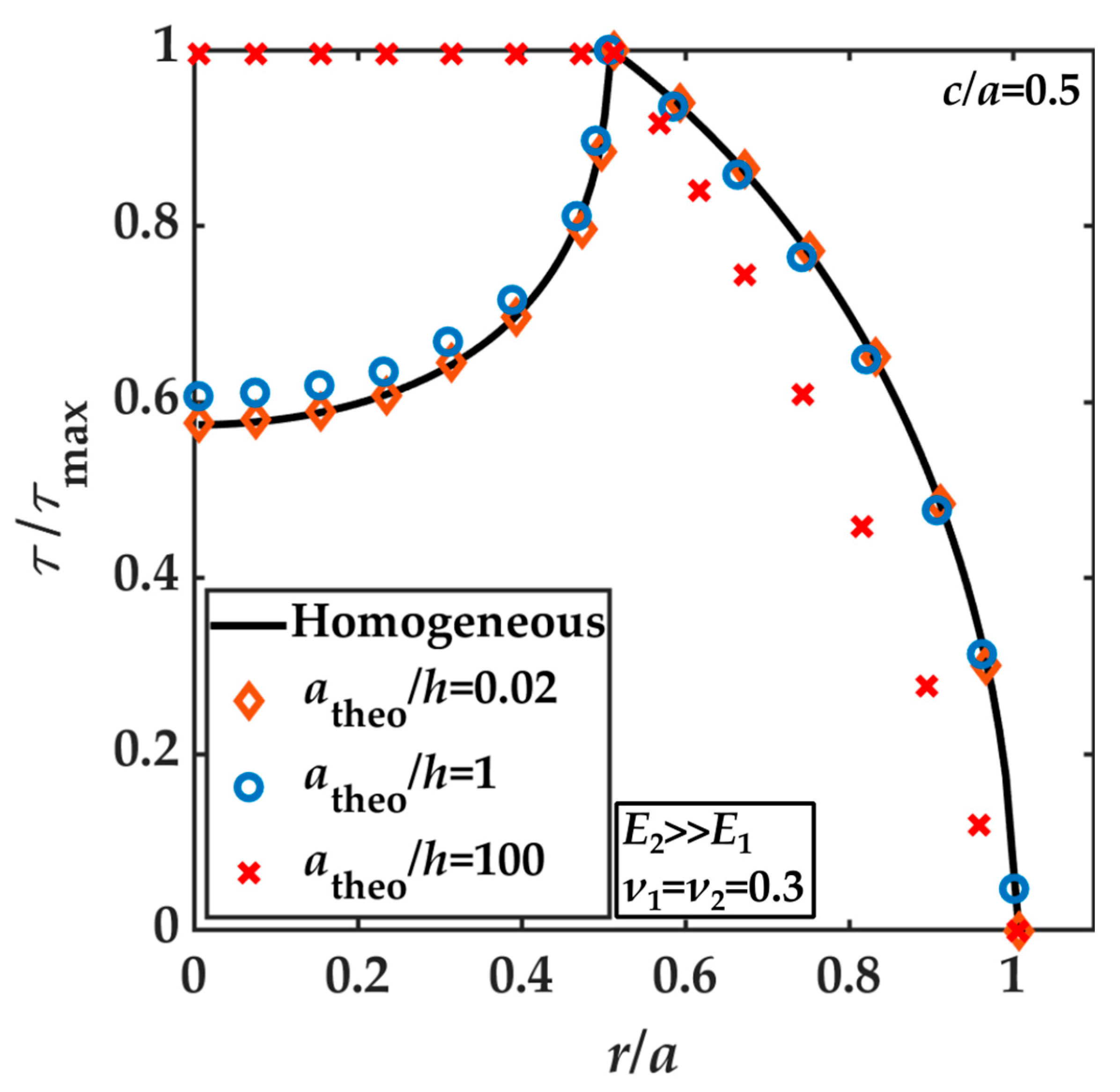
For the same values of $a_{\mathrm{theo}}/h$, the tangential stress distributions normalized to their maximum are plotted against the radial coordinate normalized to the contact radius $a$ and represented by markers (see Figure 7). In addition, the homogeneous case is plotted and represented by a solid line. As before, the homogeneous case can be represented very well by the result of $a_{\mathrm{theo}}/h=0.02$. Even for $a_{\mathrm{theo}}/h=1$ there is no big difference to the homogeneous case with the used normalizations, especially in the slip region. The course for a very thin layer $\left(a_{\mathrm{theo}}/h=100\right)$ looks quite different. In the stick region the tangential stress is constant, which is in very good agreement with Equation (64), in which no dependency on the ratio $r/a$ is given. Thus, the tangential stress distributions of the BEM results and the limiting cases can also be successfully compared using the above assumptions.

4. Conclusions

The derivation of a fundamental solution for the calculation of the tangential contact of a coated elastic half-space and its integration into the boundary element method are presented. To make the integration as simple as possible, the solution was derived in Fourier space. It is assumed that the layer is bonded to the substrate and there is no normal load to consider. The main conclusions are as follows:

• The derived solution works very well, as comparison with asymptotic analytical solutions for a very thin and a very thick layer, as well as with FEM results for finite layer thicknesses, shows very good agreement.
• With the new formulation, tangential contact problems between an arbitrarily shaped indenter and an elastic half-space coated with a layer with different elastic properties can be simulated and computed. In addition, arbitrary tangential loads can be considered.
• It might be interesting to take a closer look at the findings that have been pointed out and briefly discussed.
• Some strong assumptions, such as decoupling, Cattaneo-Mindlin and Ciavarella-Jäger, are used to study the stick-slip regions of a parabolic indenter. A study without these assumptions, that is with accounting of coupling terms and considering the direction of the displacements and the frictional force will be presented in a separate publication.

References

1. Bhushan, B.; Peng, W. Contact Mechanics of Multilayered Rough Surfaces. Appl. Mech. Rev. 2002, 55, 435–480. [Google Scholar] [CrossRef]
2. Khadem, M.; Penkov, O.V.; Yang, H.; Kim, D. Tribology of multilayer coatings for wear reduction: A review. Friction 2017, 5, 248–262. [Google Scholar] [CrossRef] [Green Version]
3. Jaffar, M.J. Asymptotic behaviour of thin elastic layers bonded and unbonded to a rigid foundation. Int. J. Mech. Sci. 1989, 31, 229–235. [Google Scholar] [CrossRef]
4. Persson, B.N.J. Contact Mechanics for layered materials with randomly rough surfaces. J. Phys. Condens. Matter 2012, 24, 10. [Google Scholar] [CrossRef]
5. Li, S.; Yuan, W.; Ding, Y.; Wang, G. Indentation load-depth relation for an elastic layer with surface tension. Math. Mech. Solids 2019, 24, 1147–1160. [Google Scholar] [CrossRef] [Green Version]
6. Westmann, R. Layered Systems Subjected to Asymmetric Surface Shears. Proc. R. Soc. Edinburgh Sect. A Math. Phys. Sci. 1963, 66, 140–149. [Google Scholar] [CrossRef]
7. Fabrikant, V. Tangential contact problem for a transversely isotropic elastic layer bonded to an elastic foundation. J. Eng. Math. 2011, 70, 363–388. [Google Scholar] [CrossRef]
8. O’Sullivan, T.C.; King, R.B. Sliding Contact Stress Field Due to a Spherical Indenter on a Layered Elastic Half-Space. J. Tribol. 1988, 110, 235–240. [Google Scholar] [CrossRef]
9. Wang, Q.; Sun, L.; Zhang, X.; Liu, S.; Zhu, D. FFT-Based Methods for Computational Contact Mechanics. Front. Mech. Eng. 2020, 6, 61. [Google Scholar] [CrossRef]
10. Pohrt, R.; Popov, V.L. Adhesive Contact Simulation of Elastic Solids Using Local Mesh-Dependent Detachment Criterion in Boundary Elements Method. Facta Univ. Ser. Mech. Eng. 2015, 13, 3–10. [Google Scholar]
11. Li, Q.; Popov, V.L. Boundary element method for normal non-adhesive and adhesive contacts of power-law graded elastic materials. Comput. Mech. 2018, 61, 319–329. [Google Scholar] [CrossRef]
12. Chen, Z.; Etsion, I. Recent Development in Modeling of Coated Spherical Contact. Materials 2020, 13, 460. [Google Scholar] [CrossRef] [Green Version]
13. Shisode, M.P.; Hazrati, J.; Mishra, T.; de Rooij, M.B.; van den Boogaard, A.H. Semi-analytical contact model to determine the flattening behavior of coated sheets under normal load. Tribol. Int. 2020, 146, 106182. [Google Scholar] [CrossRef]
14. Chen, Z.; Goltsberg, R.; Etsion, I. A universal model for a frictionless elastic-plastic coated spherical normal contact with moderate to large coating thicknesses. Tribol. Int. 2017, 114, 485–493. [Google Scholar] [CrossRef]
15. Li, Q.; Pohrt, R.; Lyashenko, I.A.; Popov, V.L. Boundary element method for nonadhesive and adhesive contacts of a coated elastic half-space. Eng. Tribol. 2019, 234, 73–83. [Google Scholar] [CrossRef] [Green Version]
16. Wang, Z.J.; Wang, W.Z.; Wang, H.; Zhu, D.; Hu, Y.Z. Partial Slip Contact Analysis on Three-Dimensional Elastic Layered Half Space. ASME J. Tribol. 2010, 132, 021403. [Google Scholar] [CrossRef]
17. Jin, F.; Wan, Q.; Guo, X. Plane Contact and Partial Slip Behaviors of Elastic Layers with Randomly Rough Surfaces. ASME J. Appl. Mech. 2015, 82, 091006. [Google Scholar] [CrossRef]
18. Komvopoulos, K. Finite Element Analysis of a Layered Elastic Solid in Normal Contact with a Rigid Surface. ASME J. Tribol. 1988, 110, 477–485. [Google Scholar] [CrossRef]
19. Popov, V.L.; Heß, M.; Willert, E. Handbook of Contact Mechanics—Exact Solutions of Axisymmetric Contact Problems; Springer-Verlag GmbH: Heidelberg, Germany, 2018; pp. 127–141. [Google Scholar]
20. Zhao, Y.; Liu, H.C.; Morales-Espejel, G.E.; Venner, C.H. Response of elastic/viscoelastic layers on an elastic half-space in rolling contacts: Towards a new modeling approach for elastohydrodynamic lubrication. Tribol. Int. 2023, 186, 108545. [Google Scholar] [CrossRef]
21. Cattaneo, C. Sul Contatto di due Corpore Elastici: Distribuzione degli sforzi. Rend. Dell’ Acad. Naz. Dei Lincei 1938, 27, 342–348. [Google Scholar]
22. Mindlin, R.D. Compliance of elastic bodies in contact. J. Appl. Mech. 1949, 16, 259–268. [Google Scholar] [CrossRef]
23. Jäger, J. A New Principle in Contact Mechanics. J. Tribol. 1998, 120, 677–684. [Google Scholar] [CrossRef]
24. Ciavarella, M. Tangential Loading of General Three-Dimensional Contacts. J. Appl. Mech. 1998, 65, 998–1003. [Google Scholar] [CrossRef] [Green Version]
25. Dassault Systems Simulia Corp. SIMULIA User Assistance; Dassault Systems Simulia Corp.: Providence, RI, USA, 2021. [Google Scholar]
Figure 1. A schematic representation of a coated body. The elastic constants of the layer are E 1 and ν 1 while those of the half-space are E 2 and ν 2 . The thickness of the layer is h and the coordinate origin is on the outer surface of the coating.
Machines 11 00694 g001
Figure 2. Representation of the mesh used for the numerical simulation. An area is shown enlarged to illustrate the discretization and, by way of example, the stress in a cell.
Machines 11 00694 g002
Figure 3. Representation of the new coordinate system x , y , which is rotated relative to x , y by the angle φ .
Machines 11 00694 g003
Figure 4. The normalized tangential contact stiffness k T , n o r m plotted against the ratio of elastic moduli E 1 / E 2 for different ratios a / h . The BEM solutions are represented by different types of lines for the different ratios a / h . The FEM solutions are represented by markers that have the same color as the corresponding line. The Poisson’s ratio of the layer and the substrate are ν 1 = ν 2 = 0.3 .
Machines 11 00694 g004
Figure 5. Comparison between the BEM results (solid lines) and analytical results of the limiting cases (dotted and dashed lines) for different ratios a / h and for two different ν 1 . The elastic modulus of the substrate is much larger than that of the layer E 1 / E 2 = 10 9 .
Machines 11 00694 g005
Figure 6. The ratio of radii c / a plotted against the ratio u x / u x , max . The analytical results of the limiting cases (solid and dashed lines) are compared with the BEM results (markers) for different ratios a theo / h . The elastic parameter data are given and the contact configuration at c / a = 0.5 for a theo / h = 1 is shown as an inset image.
Machines 11 00694 g006
Figure 7. Tangential stress distributions at c / a = 0.5 for different ratios a theo / h , plotted against the ratio r / a , normalized to its maximum and represented by markers. The homogeneous case is represented by a solid line. Information on the elastic parameters is given.
Machines 11 00694 g007
Disclaimer/Publisher’s Note: The statements, opinions and data contained in all publications are solely those of the individual author(s) and contributor(s) and not of MDPI and/or the editor(s). MDPI and/or the editor(s) disclaim responsibility for any injury to people or property resulting from any ideas, methods, instructions or products referred to in the content.