Article

Hardware-in-the-Loop Scheme of Linear Controllers Tuned through Genetic Algorithms for BLDC Motor Used in Electric Scooter under Variable Operation Conditions

by
Leonardo Esteban Moreno-Suarez
,
Luis Morales-Velazquez
,
Arturo Yosimar Jaen-Cuellar
and
Roque Alfredo Osornio-Rios
*
Cuerpo Académico (CA) Mecatrónica, Facultad de Ingeniería, Universidad Autónoma de Querétaro, Av. Río Moctezuma 249, San Juan del Río, Querétaro 76807, Mexico
*
Author to whom correspondence should be addressed.
Machines 2023, 11(6), 663; https://doi.org/10.3390/machines11060663
Submission received: 4 May 2023 / Revised: 13 June 2023 / Accepted: 16 June 2023 / Published: 19 June 2023
(This article belongs to the Special Issue Condition-Based Monitoring of Electrical Machines)

Abstract

:
Outrunner brushless DC motors (BLDC) are a type of permanent magnet synchronous motor (PMSM) widely used in electric micro-mobility vehicles, such as scooters, electric bicycles, wheelchairs, and segways, among others. Those vehicles have many operational constraints because they are driven directly by the user with light protective wearing. Therefore, to improve control strategies to make the drive safer, it is essential to model the traction system over a wide range of operating conditions in a street environment. In this work, we developed an electro-mechanical model based on the Hardware-in-the-Loop (HIL) structure for a two-wheeler electric scooter, using the BLDC motor to explore its response and to test linear controllers for speed and torque management under variable operating conditions. The proposed model includes motor parameters, power electronics component characteristics, mechanical structure, and external operating conditions. Meanwhile the linear controllers will be adjusted or tuned though a heuristic approach based on Genetic Algorithms (GAs) to optimize the system’s response. The HIL scheme will be able to simulate a wide range of conditions such as user weight, slopes, wind speed changes, and combined conditions. The designed model can be used to improve the design of the controller and estimate mechanical and electrical loads. Finally, the results of the controller tests show how the proposed cascade scheme, tuned through the GA, improves the system behavior and reduces the mean square error with respect to a classical tuning approach between 20% and 60%.

1. Introduction

The micro-mobility is a topic focused in the society welfare that has been gaining attention in recent years due to the combination of aspects such as fast urbanization, climate change, population growth, and the need of efficient and ecological innovative systems for people movement [1]. Thus, problems such as public transport pollution, insufficient variety of sustainable public transport, and city traffic issues have brought the opportunity to explore the use of vehicles that represent alternative methods for mobility such as those that are fully electric [2] and with regenerative energy features [3]. Thus, the micro-mobility is the expression assigned to vehicles characterized by their compact design, with light weights, achieving low velocities (generally under the 30 km/h similar to bicycles) that are driven exclusively by the road users (nobody else) [4]. In this sense, the devices used for micro-mobility encompass bicycles, e-bikes, electric scooters, electric skateboards, shared bicycles, and electric pedal-assisted bicycles [5]. Some of the aforementioned devices rely in what is known as active mobility, or active travel, which considers all models of transport that are based on the propulsion generated by human power [6]. However, the interest in this work is in those devices that make use of electric power. For example, the electric scooter is of special interest because of its popularity, ease of access, low-to-medium cost, ease of carrying and transporting, the velocities that can be reached, the green mobility over short-to-medium distances, effortless use, the parallel possibility of using other types of transport, less requirements for parking and space, and some others [7]. The electric scooter integrates several components such as the mechanical structure, the electronics and drivers, the batteries, the system controllers, and the motor; the last is typically a brushless direct current (BLDC) motor [8]. Despite its advantages, some elements in the scooter still require attention, such as the embedded controllers and the BLDC motor, to raise its efficiency as much as possible and for keeping the system security, maintaining a constant velocity, and reducing the energy consumption [9]. This is because the design of the electric scooter does not consider all the possibilities in the final operation conditions such as weight variations, path rugosity, slopes in the path, affectations derived by wind speed, among others. Additionally, another important aspect to meet with the requirements of velocity and performance is the use of banks of batteries, and they must be managed adequately in aspects such as storage, distribution, operation, and energy savings [10]. Therefore, an adequate control scheme to maintain, for instance, a defined velocity and torque under these changing conditions, optimizing the energy consumption from the batteries, is essential and still represents an area of opportunity. Additionally, these controllers require more complete and integrated system models, which, in several cases, are not easy to obtain.
With the purpose of designing a control scheme is necessary to use a system model, an appropriate model of the electric scooter is required in order to propose improvements in the system’s dynamics, controls, and design [11]. For example, the work proposed in [12] presents the development of an electric two-wheeler numerical model, considering the energy-conservation-based longitudinal dynamic coupled to a Li-Ion battery second-order RC equivalent circuit to predict the electric range under real driving cycles. By its part, the investigation carried out in [13] described an specific design of an electric three-wheeled scooter for being used by persons with partial incapacities to move. For such design, the proposed model was performed through Solidworks, considering a hub motor, battery, and control system that achieved velocities up to 45 km/h and a carrying load capacity of 100 kg by simulation. In other cases, such as in [14], an adaptive Cuckoo search (ACS) is combined with the extreme learning machine (ELM) for developing a prognosis method of the remaining useful life of intermittently fault components of an electric scooter system. To perform the prognostic, first, a diagnostic bond graph (DBG) model of the electric scooter was developed, later sub models were obtained through structural model decomposition, the ACS estimated distributed faults, and the ELM modeled the intermittent fault degradation. In another case, the research presented in [15] described the energy optimization of a two-wheeler hybrid electric vehicle (HEV). First, a through-the-road (TTR) parallel HEV system structure was proposed and modeled, and then three control strategies were switched, considering the state of the charge, fuzzy logic, and a neural network. The comparison of the strategies was performed under the Simulink environment and under simulations in a world-harmonized motorcycle test cycle (WMTC) drive cycle. In other works, the analyses, modeling, and designs of specific parts used in electric scooters are addressed, such as the case of the design and optimization of a switched reluctance motor (SRM) developed in [16]. To achieve this design, the analysis of the SRM configuration with 8 and 10 poles on the stator and rotor was performed through two-dimensional electromagnetic static finite element analysis combined with multi-objective design optimization (MOO) and particle swarm optimization (PSO). The works previously discussed clearly indicated that research addressing systems modeling could be useful for the development of methodologies that improve such systems behaviors, without compromising the integrity of a physical system.
In recent years, a relatively new concept, known as hardware-in-the loop (HIL), has taken the old definition of simulation to a new level because it incorporates physical hardware systems as integral parts of a large simulation system [17]. This tool can be very helpful for experimenting and validating developed methodologies and designs in a wide variety of applications such as approaches for modeling electric machine drives [18], the development of electrical test benches for drive inverters in the power electronics field [19], studies of the impact of smart appliances connected to the electric grid [20], applications for designing new automotive products with vision systems for efficient software validation [21], and automotive applications in general for modeling electric vehicles [22], among others. The HIL simulation has been used for modeling, analyzing, and designing electric vehicles. For instance, the work described in [23] presented an intelligent controller for an HEV. In the work, a model predictive controller (MPC) was enhanced though an artificial neural network (ANN) for controlling the speed of the HEV, and the simulation model and a HIL system were implemented with Simulink on MATLAB (https://www.mathworks.com/, accessed on 1 May 2023). This controller was compared with classical controllers such as a linear Proportional + Integral (PI) and with a classic MPC. However, some limitations could be mentioned, such as the use of a low-cost Arduino Mega 2560 platform, which had low performance for hardware applications, and it was only used for communication and signal transmission functions in the closed loop (as the model and the controller were implemented in Simulink). Additionally, the way in which the classical controllers were tuned or adjusted was not detailed for the comparison. Additionally, only one control variable was considered, which was the system velocity analyzed under two case studies: variations in the controller reference and noise rejection of the controller. Finally, the model considered parameters for the motor, the engine, the tires, the system drive, the DC-to-DC converter, the vehicle body, and the battery, but it did not consider the effects of the environment such as wind speed, path profiles and slopes, variations in the system mass, etc. Regarding the use of HIL, a real-time implementation into a field-programmable gate array (FPGA) of a vector control scheme was performed in [24]. In that work, the control scheme, integrated by three PI controllers, was applied to a permanent magnet synchronous motor (PMSM) that propelled an electric scooter. The models of the PMSM and the converter were implemented in MATLAB Simulink, whereas the control scheme was developed through Xilinx System Generator (XSG) without Hardware Description Language (HDL) coding. Thus, the HIL was a co-simulation between the FPGA and Simulink. However, some limitations could be mentioned. For example, the use of the vector control scheme for the speed control was not justified, and the method for tuning the proportional and integral gains was not detailed. The system model only considered the parameters of the PMSM, and the other elements of the scooter were fixed, such as mass and load. Finally, the control of the modeled system was analyzed, considering a fixed velocity reference from the New European Duty Cycle (NEDC), and the highway section of the cycle was not considered. In this same line, a HIL platform was developed in [25] for a hybrid electric scooter (HES) with the purpose of using a fuzzy control that managed three power sources. The dynamic of the HES was of a low-order but considered several subsystems such as a spark–ignition engine, a high-power traction motor, an integrated starter generator, a high-power battery module, transmission, and a longitudinal vehicle dynamic. Nonetheless, some drawbacks were observed, such as the 73 inference rules for fuzzy control, which were classically defined for the seven operation modes without adaptability of the rules and requiring expert knowledge for defining them. Additionally, the operating conditions of the considered model were fixed as constant, limiting the analysis of the system’s response under realistic environments. Finally, only the speed of the HEV was considered as the control variable, despite the different feedback signals based on torque to indirectly define the vehicle’s speed. From the reported literature, the HIL systems were excellent tools that allowed effective testing of their analogous physical systems (without having the real system itself). They could include elements or parts that analytical modeling could not, which were excellent characteristics if rapid developments requirements were demanded. Nevertheless, some aspects are still required to be addressed, such as the type of control strategy, its design and tuning, and the modeling of the systems because it still assumes some conditions as constant or negligible, etc.
From the analysis of the works reported in the literature, it can be observed that most of the models used for describing the physical systems are analytical, and, normally, they do not represent the complete system. In many cases, the model is focused on a specific part or element, for instance, the motor, the drivers, the converter, etc. By its part, the models that consider a complete electric vehicle system are very complex, their implementation is far from reality, and they are limited because they do not consider variations in their parameters during operation and dynamic simulation. For example, during the model design of an integrated electric vehicle, some operating parameters are assumed as constant values, such as weight and a flat path, with the purpose of reaching a desired velocity and torque of the vehicle on its way. Another aspect is that many models are validated by simulation, and, in some cases, it is very complex to analyze realistic conditions. In this sense, the HIL systems can be an effective tool for addressing a simulation from a real perspective, and this is similar to what is known as digital twins, where a digital system is compared with the physical system for deep analysis.
The contribution of this work is the development of a model based on the Hardware-in-the-Loop (HIL) structure for a two-wheeler electric scooter, considering several changing operating conditions of the system. The model of the physical scooter considers the mechanical and the electrical parts as several subsystems such as the brushless direct current (BLDC) motor, the power inverter of the motor based on a bidirectional converter, the mechanical structure, the battery, etc. By its part, between the operating conditions that will be analyzed in the proposed model are the effects in the dynamics due to the masses of both the user and the mechanical structure, the motor speed and torque, the path profiles or conditions such as slopes, and the effects in the aerodynamics due to environmental factors such as wind speed. Further important aspects in the proposed HIL approach are the control structures applied for the proper operation of the electric scooter on the bidirectional converter and for the compensation to the motor in order to achieve the desired velocity and torque when an operating condition changes. It must be highlighted that the controller’s tuning is carried out through a heuristic approach based on genetic algorithms (GAs). Four case studies, where variations in the wind speed, the mass of the system, path profile variation, and combined conditions are analyzed. The obtained results through the HIL platform demonstrate that the optimization scheme on the system controllers allow the improvement of the operation of the electric scooter without compromising the integrity of a physical system and its security aspects.

2. Materials and Methods

In the following subsections, the theoretical foundations and the methodology followed for the development of the HIL platform for a two-wheeler electric scooter considering changing operating conditions of the system will be described.

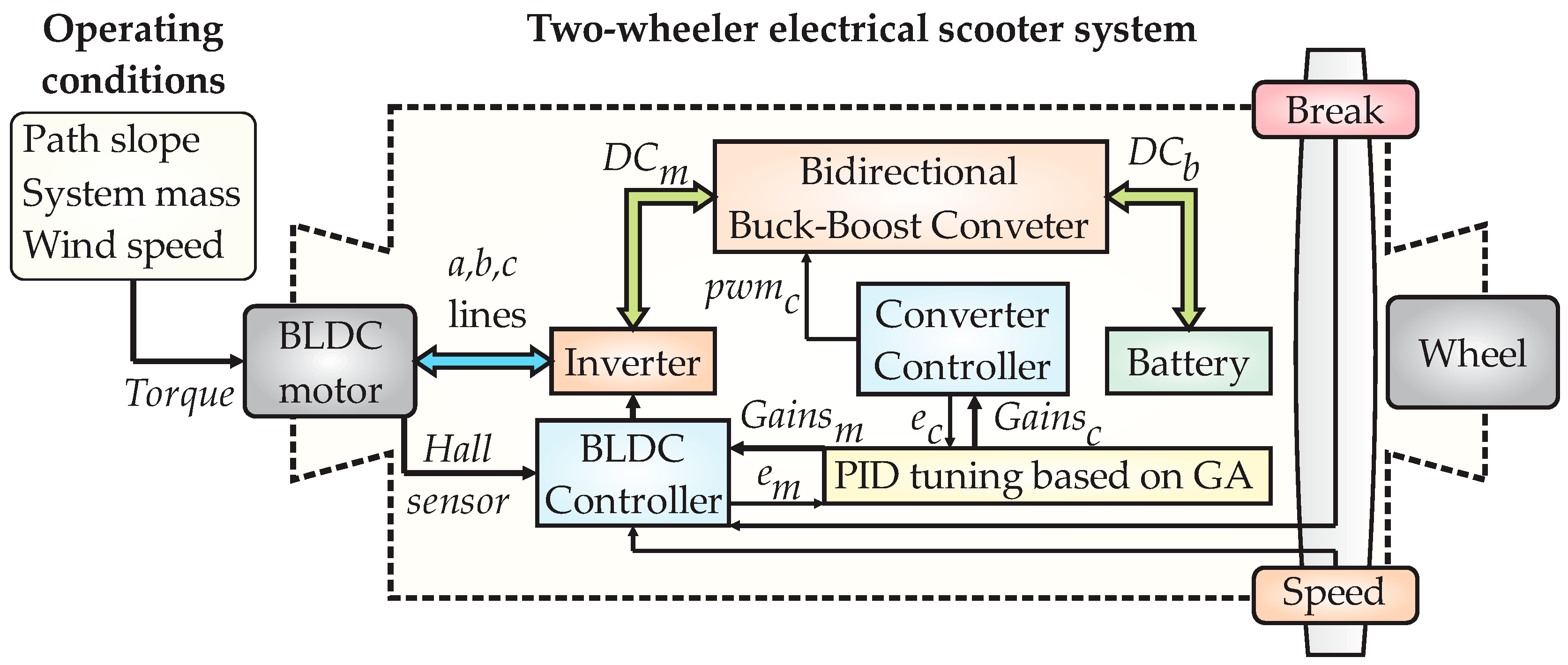
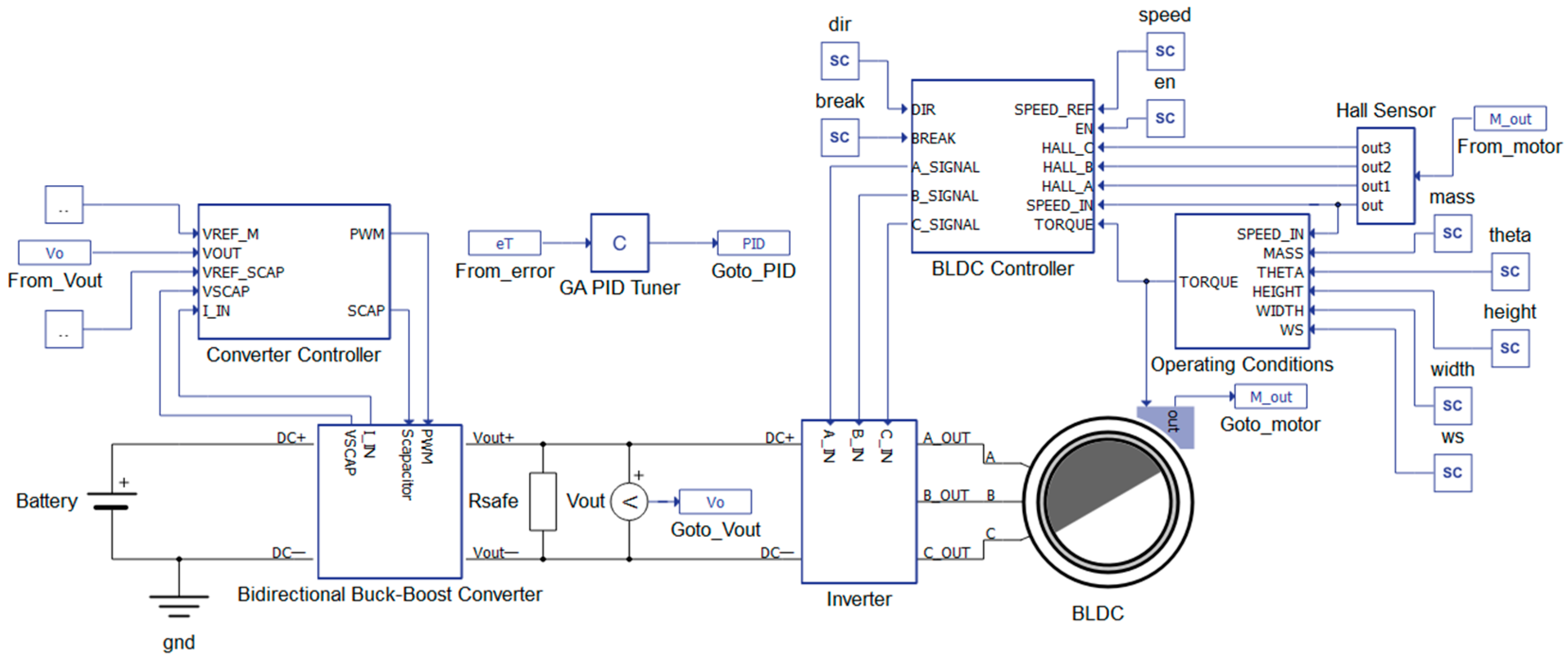
2.1. Two-Wheeler Electrical Scooter Model

Figure 1 shows a general block diagram remarking on two main parts considered in the proposed HIL platform such as (i) the operating conditions and (ii) the system of the two-wheeler electric scooter.
From Figure 1, the first block of the proposed HIL system is the operating conditions. The conditions are determined by the forces interacting with the electric scooter’s displacement, such as the friction force generated between the wheel and the path relief, the resistance caused by the wind speed, and the acceleration force required by the vehicle to keep the movement. These operating conditions consider the parameters of the system mass, the wind speed, and the path slope (inclination angle with respect to the horizontal plane) as inputs. Regarding the path slope, this parameter implies the possible presence of the slopes in the path that the two-wheeler electric scooter can face, affecting the speed and the torque directly. Therefore, the scooter must be capable of compensating for the effects of the system’s operation due to the slopes and their inclinations; naturally, it is expected that the velocity must be guaranteed as constant when a slope appears in the trajectory of the scooter. In relation to the system mass, this parameter considers both the mass of the mechanical structure (including the batteries with the other subsystems) and the mass of the user driving the electric scooter. The total mass is analyzed from the viewpoint of the affectations in the system’s dynamic behavior when this parameter is changed because the mass variations could be assumed as very insignificant in real conditions. By its part, the wind speed parameter implies the affectation in the system displacement velocity due to the aerodynamics modified by the user through their width and height.
The second block of the diagram is the two-wheeler electric scooter that was integrated by several subsystems: the battery, bidirectional buck-boost converter, inverter, BLDC motor, converter controller, BLDC controller, PID tuning based on genetic algorithms (GAs), and wheel. A lithium battery was chosen for the voltage and current source used for feeding the electric scooter. The battery had a capacity of 24 V and 30 A. Thus, the battery provided the voltage D C b for the bidirectional buck-boost converter but also the battery received the recovered energy through the regenerative braking. On the other side, the bidirectional buck-boost converter was a type of DC-to-DC converter that operated in two ways: the boost mode (the voltage was increased) and the buck mode (the voltage was reduced). In the boost mode, the converter received the supplied voltage by the primary source, which was the battery, and its purpose was raising the voltage up to 48 V, which fed the inverter, keeping a constant value, allowing the BLDC motor to work on propelling the scooter. Meanwhile, in contrast, the buck mode worked when the electric vehicle needed to slow down or brake, allowing the recovery of the mechanical energy converted to electrical energy because the motor operated similar to a generator, being a secondary source of the converter. Then, the electrical energy recovered remained constant despite the changes produced in the supplied voltage by the motor, keeping the potential difference of the battery. The bidirectional connection between the buck-boost converter and the inverter was represented as D C m . Now, regarding the inverter, it performed the voltage conditioning from direct current (DC) to alternating current (AC) in three lines. This signal conditioning was performed through the H-bridge structure by using metal-oxide semiconductor field effect transistors (MOSFETS) with high powers for feeding a sinusoidal wave voltage signal to each one of the three motor windings, represented as A , B , C lines. Regarding the BLDC motor, this was a type of permanent magnet electric machine, with direct traction and an outer rotor coupled to the electric vehicle wheel, having high torque and allowing for the energy recovery. The internal hall sensors allowed the adequate commutation of the BLDC motor through the inverter and provided information about its rotation direction. Now, for the case of the converter controller subsystem, it was in charge of generating the pulse width modulation signal p w m c required by the bidirectional converter with the purpose of operating in the modes buck or boost. To achieve this, the controller was implemented as a cascade scheme with Proportional + Integral + Derivative (PID) actions to accomplish a level current and voltage required by the bidirectional converter. This way, the internal closed-loop applied a PID control for the current, and the external closed-loop applied a PID control for the voltage. By its part, the BLDC controller subsystem was in charge of achieving the desired velocity and torque in the motor. To meet this goal, the control scheme was also a cascade structure, being the internal PID loop dedicated to the torque and the external PID loop to the velocity. Last but not least, the PID tuning based on the GA adjusted the gains of the controllers through a heuristic approach, where the signal error of the voltage and current e c and the error of the torque and velocity e m achieved were used in the objective functions for the gain’s adjustment. The outputs of this subsystem were the optimized gains for the controller converter G a i n s c and the gains for the BLDC controller G a i n s m .

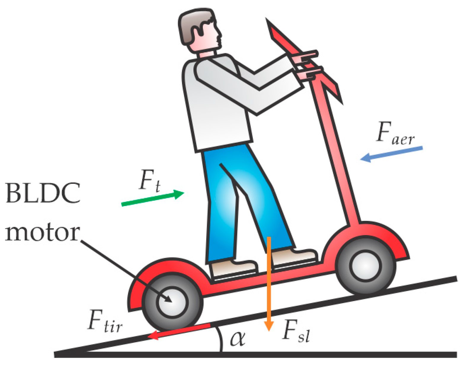
2.2. System Dynamics Modeling

As it was mentioned, the two-wheeler electric scooter was integrated by several subsystems to know the battery, bidirectional buck-boost converter, inverter, BLDC motor, converter controller, BLDC controller, the tuning based on genetic algorithms (GAs), and the wheel. In this section, the analytic models of some of the subsystems in Figure 1 will be explained in detail, as these models were implemented in the HIL platform. Hence, beginning with the electric model of the BLDC motor that had a three-phase “Y” configuration in the stator windings [26], which is presented in expression (1):
V a V b V c = R a 0 0 0 R b 0 0 0 R c i a i b i c + L M 0 0 0 L M 0 0 0 L M d d t i a i b i c + e a e b e c
where the parameters involved in the motor dynamics are the phase voltages V a , V b , and V c ; the stator winding resistances R a , R b , and R c ; the stator currents i a , i b , and i c ; the stator inductance L ; the mutual inductance between the stator windings M ; and the electromotive forces e a , e b , and e c . Now, the corresponding mechanical model of this BLDC motor [26] is presented in Equation (2):
T e = T L + J · d ω m d t + B · ω m
where T e is the motor torque with units in N · m ; T L is the load torque applied to the motor with units in N · m ; J is the inertia moment expressed in k g · m 2 / r a d ; ω m is the angular velocity of the motor measured in r a d / s ; and B is the friction constant of the motor.
To obtain the transfer function of the BLDC wheel motor, a phases conduction must be considered, for instance, between phases a and b ; therefore, i a = i b = i , where i is the current that flows between both phases [27,28]. This way, taking the currents from expression (1), the voltage between the phases a and b was obtained through Equation (3):
V a , b = R a + R b · i + 2 · L M · d i d t + e a + e b
When both phases were active, they were equal in magnitude but with opposite directions; thus, (3) can be rewritten through (4), as follows:
V a , b = 2 · R · i + 2 · L M · d i d t + 2 · e U = R l · i + L l · d i d t + k e · ω m
where U is the applied voltage to the motor; R l is the resistance; L l is the inductance; and e is the electromotive force. All of these values were considered between the two phases. Additionally, the product of the angular velocity ω m of the motor with the back-electromotive force constant k e was the electromotive force e , according to the analogy in (4). By the other side, the motor torque could also be obtained by means of the torque constant k T and the current between the phases i [29], as observed in (5):
T e = k T · i
Next, by substituting (5) in (2), we have the expression of (6):
k T · i = T L + J · d ω m d t + B · ω m
Then, by assuming the relation of (6) with a torque of the motor under no load condition ( T L = 0 ), with the purpose of obtaining the system model without external affectations, it was possible to obtain the value of the current, as indicated in (7):
i = J k T · d ω m d t + B k T · ω m
Now, the current i of (7) could be substituted in the equality of the right side in expression (4). Thus, by applying the Laplace transform to the resulting expression, the transfer function of the motor G ( s ) is the ratio between the output, angular velocity ω m ( s ) , input, and applied voltage U (s) [28], yielding the system model observed in (8):
G s = ω m ( s ) U ( s ) = k T L l · J · s 2 + R l · J + L l · B · s + R l · B + k e · k T
The parameters of the BLDC motor considered in this proposed work for the two-wheeler electric scooter are summarized in Table 1.

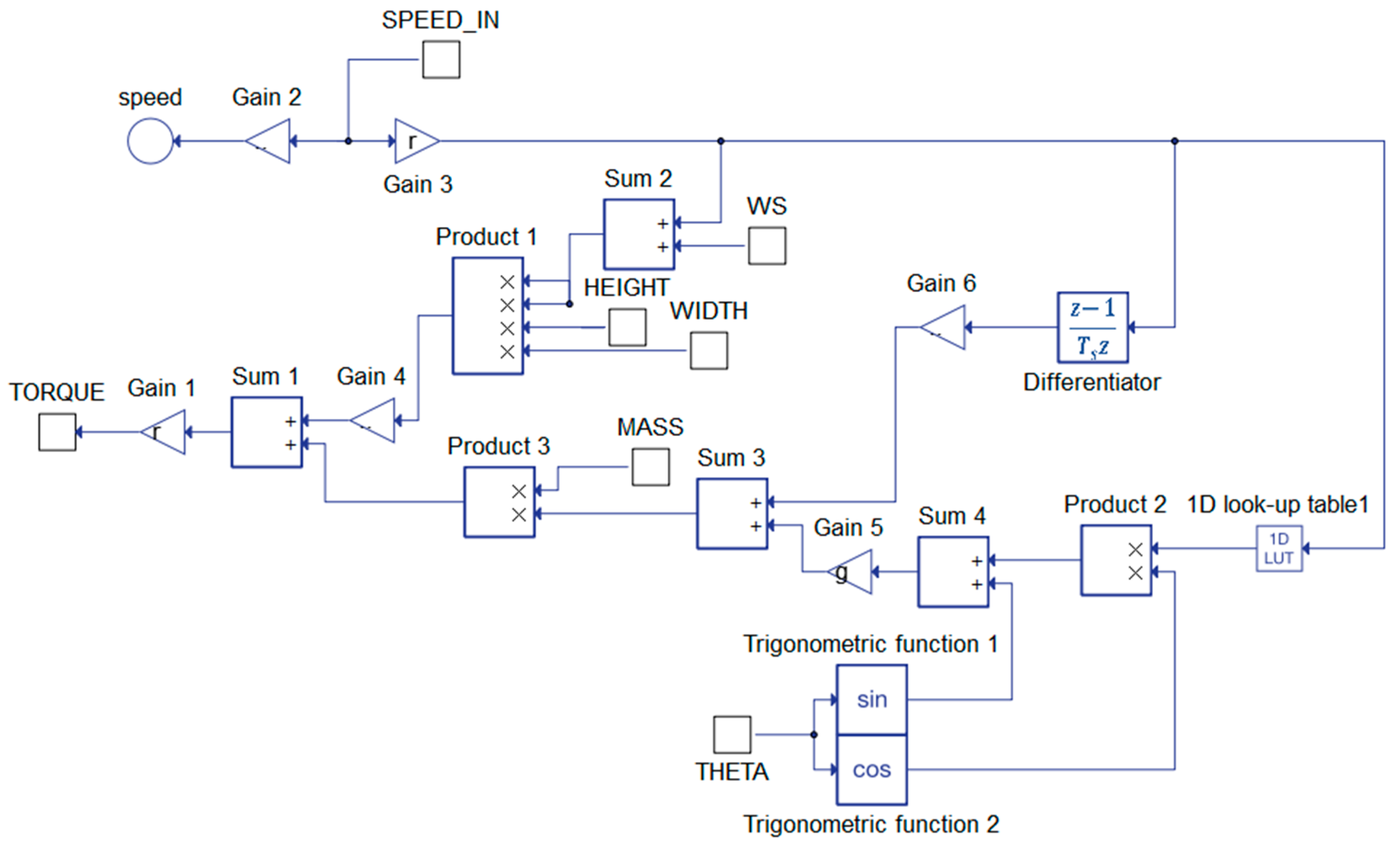
2.3. Operating Conditions Modeling

As it was previously mentioned, the two-wheeler electric scooter would be affected by external forces during the vehicle displacement. Figure 2 displays a free-body diagram of these external forces affecting the system’s dynamics, and the following expressions were obtained according to [30,31].
From Figure 2, the rolling force F t i r over the horizontal plane between the BLDC motor wheel and the path surface, where the vehicle goes on its way, can be computed through (9):
F t i r = f r · m · g · c o s α
where f r is the rolling constant force; m is the total mass of the manned vehicle; g is the standard acceleration of gravity; and α is the angle of the vehicle path with respect to the horizontal plane. Meantime, the expression to obtain the force due to the slope in the vehicle path F s l is observed in (10):
F s l = m · g · s i n α
Regarding the effects of the wind speed, when a user is driving the two-wheeler electric scooter, the wind causes a resistance in the vehicle displacement because the user characteristics, such as its height and width, modify the system aerodynamics. Thus, this resistance is a force F a e r generated because the system’s aerodynamics are changed, and its effects are considered through Equation (11):
F a e r = 1 2 · ρ a · a v · c a r · v 2
From the equation, ρ a is the air density; a v is the contact area to the wind of the vehicle; c a r is the aerodynamics resistance coefficient; and v is the linear velocity of the vehicle with respect to the wind speed.
Therefore, considering the effects of all these external forces interacting with the electrical scooter, and according to the Newton’s law, the sum of forces F s must be equal to the system mass m , multiplied by the acceleration value a , as stated in (12) and rewritten as in (13):
F s = F t F t i r F s l F a e r = m · a
F t = F t i r + F s l + F a e r + m · a
where F t represents the traction force of the motor wheel. By its part, the torque load T L , or electromagnetic torque, applied to the BLDC motor of permanent magnets with synchronous rotation can be computed by Equation (14):
T L = F t × r
where r is the motor radius because the machine is a wheel motor ensemble of direct drive traction.

2.4. Hardware-in-the-Loop Proposed Structure

In this section, the main system and the subsystems that require detailed explanation for being implemented in the HIL simulation are described: the general system structure (two-wheeler electric scooter), the operation conditions’ sub block, the converter controller sub block, and the BLDC controller sub block. Therefore, the block diagram of Figure 3 shows the complete structure of the proposed HIL for testing the linear controllers tuned by the GA applied to a two-wheeler electric scooter BLDC motor. The description of the diagram begins with the voltage source, which is the battery type lithium with 24 V and 30 A feeding the bidirectional buck-boost converter. Now, regarding the bidirectional converter sub block, the input signals received are the pulse width modulation (PWM) of the converter controller and the signal that establishes the supercapacitor’s connection, named SCAP; this last signal also performs the commutation of the MOSFETs in the converter. Meanwhile, the corresponding outputs are the digital signals that give information about the supercapacitor voltage (VSCAP) and the input inductor current (I_IN), which, in turn, are connected to the converter controller sub block. By its part into the converter controller, in addition to the feedback signals VSCAP and I_IN, other input signals are received such as the reference voltage of the super capacitor (VREF_SCAP), the reference voltage of the BLDC motor (VREF_M), and the output voltage (Vo) of the bidirectional converter; this last signal is acquired by a measurement function given by the simulation software. The corresponding output signals are the previously mentioned PWM and SCAP. It is worth mentioning that the analogic signal Vo has a protection resistance of high impedance, with the function of discharging the energy storage components of the bidirectional converter to avoid damage and errors in the measure, connected in parallel.
Posteriorly, the voltage provided by the bidirectional converter supplies the motor inverter consisting in an H-bridge arrangement of MOSFETs generating the three-phase outputs A_OUT, B_OUT, and C_OUT, which, in turn, feed the BLDC motor. The parameters defining the BLDC motor dynamics are summarized in Table 1, but also this motor includes hall effect sensors into its case, represented in the diagram as M_out, providing the information about the rotation’s synchronism. Additionally, the BLDC motor sub block receives the variations in the torque determined by the operating conditions’ sub block. Concerning this last sub block (operating conditions), it receives the parameters of the total mass (MASS), the slope angle (THETA), the user characteristics such as height (HEIGTH) and width (WIDTH), and the wind speed (WS) as inputs. The last three parameters affect the displacement because they modify or impact the vehicle’s aerodynamics. Additionally, this sub block has a feedback input of the motor velocity through the input SPEED_IN provided by the hall sensors. Now, the BLDC controller sub block receives the following inputs, the velocity (SPEED_IN) and torque (TORQUE) values of the motor, the hall sensor signals (HALL_A, HALL_B, and HALL_C), and also the external signals stablished by the user such as vehicle start (EN), the reference velocity (SPEED_REF), the motor direction (DIR), and the breaking command (BREAK). Consequently, the BLCD controller establishes the driver’s commutation per phase, providing the corresponding synchronization signals A_IN, B_IN, and C_IN to the inverter. This inverter generates the output signals A_OUT, B_OUT, and C_OUT that are sent to the BLDC motor for controlling the rotation speed and torque. Regarding this motor, the implemented model is the transfer function observed in (8) that was obtained through Equations (1)–(7). Finally, the GA PID Tuner sub block performs the adjusting of the PID controller’s gains of both the bidirectional converter and the BLDC motor, having the error sets on each control as input parameters.
The block diagram of Figure 4 shows the part of the proposed HIL structure corresponding to the generated operating conditions affecting the behavior of the electric scooter such as the external forces specified in (13), which, in turn, depend on parameters such as the wind speed, the system’s mass, and the path’s slope angle. In first place, and for visualization purposes, the vehicle velocity SPEED_IN, with original units in radians per second (rad/s), is converted through the “Gain 2” function to units in kilometers per hour (km/h) displayed on the speed view. In second place, the force F a e r of expression (13) is computed according to Equation (11) as follows. The “Gain 3” function performs the conversion of the original velocity units to meters per second (m/s), and this value is added to the wind speed value WS through the “Sum 2” addition function. This result is fed twice to the multiplication function “Product 1”, representing the velocity raised to power 2, but also the height and width of the user and the vehicle are fed to this block as a set representing the contact area exposed to the wind. Next, the air density and the aerodynamics’ resistance coefficient are considered in the function “Gain 4” to obtain the resulting force. In third place, the forces F t i r , F s l , and the term m · a are computed through a factorization of Equations (9), (10) and (13), of course without the force F a e r , as follows. The velocity of the function “Gain 3” is derivative, with respect to time, and the acceleration of the electric scooter is obtained with the function “Gain 6”. Meanwhile, this velocity is also used to specify the rolling constant force through the lookup table function “1D look-up Table 1”. Additionally, the “1D look-up Table 1” function defines the effects of the grounding friction force indirectly through the rolling constant force on the tire, caused by a change in the type of surface material on which the tire is rolling to. This look-up-table changes the rolling constant force, considering the grounding friction on the tire, depending on the vehicle speed and the type of surface (pavement, wood, dirt road, wet surface, etc.). By its part, the path slope angle is input to compute the sine and cosine values through the functions “Trigonometric function 1” and “Trigonometric function 2”, respectively. Regarding the cosine value, this is multiplied by the rolling constant force in the function “Product 2”, whose output is added to the sine value in the function “Sum 4”. This addition is multiplied by the standard acceleration of gravity through the function “Gain 5”, added to the vehicle acceleration in the function “Sum 3” and multiplied by the system mass in the function “Product 3”. In fourth place, the summatory of the forces F a e r , F t i r , F s l , and the term m · a (traction force of the motor wheel) is obtained through the function “Sum 1” and multiplied by the motor radius through the cross product by means of the function “Gain 1” to obtain the torque load T L applied to the BLDC motor, according to (14).
In Figure 5, the part of the proposed HIL corresponding to the bidirectional buck-boost converter controller is presented. This sub block has input data such as the desired voltage in the super capacitor VREF_SCAP and the feedback of the value of charged VSCAP. Thus, the difference between VREF_SCAP and VSCAP generates a signal error by means of the function “Sum 3”, which is connected to a PID controller considered for the buck mode of the converter. It is worthwhile to mention that this controller is isolated from those tuned by means of the GA approach, which means that this PID has fixed gains obtained through the empirical rules of Ziegler–Nichols because the operating conditions do not affect the converter in the buck mode since the motor is the energy source connected to the battery. The controller output is enabled through the function “Signal Switch 1”, which, in turn, is activated by the logic gates NOT and OR responding to the input source “buck”; this input defines the operation mode of the converter. Now, the controller output is compared in the function “Comparator 2” with a triangle waveform of the function “Triangular Wave Source 1” for generating the pulse width modulation (PWM) that is joined in the function “PWM Bus”. This PWM signal is used for maintaining the supercapacitor voltage of the bidirectional converter as constant as possible in the desired value required for its adequate internal operation. On the other hand, it is very important to mention that the voltage and current provided by the battery (24 V and 30 A) are increased to 48 V by the demanded current of the BLDC motor depending on the vehicle load in the converter boost mode. Therefore, to achieve these goals, a cascade control scheme of two PID regulators is implemented, being the internal PID loop applied to the control of the demanded current by the motor, and the external PID loop is applied to maintain the constant 48 V that could vary because of the operating conditions. The cascade control begins in the external loop with the inputs of the converter voltage reference VREF_M (48 V) and the voltage feedback of the converter VOUT, which are used to generate an error signal in the function “Sum 1” for feeding the controller “Voltage PID Controller”. It must be noted that the voltage error signal, stored in the global variable “eT”, will be sent to the sub block “GA PID Tuner” for the respective tuning process. Next, in the cascade scheme, the controller output of the external loop will be used as the new reference for the internal loop, then the real demanded current input I_IN is used to generate a signal error in the function “Sum 2” for feeding, in this case, the controller “Current PID Controller”. Similarly, as in the case of the voltage signal error, the current signal error, also stored in the global variable “eT”, will be sent to the “GA PID Tuner” sub block. Additionally, the final output of the cascade control is compared in the function “Comparator 1” with a triangle waveform of the function “Triangular Wave Source 2” for generating the respective PWM that will be joined in the function “PWM Bus”. However, this PWM signal is enabled, and the PID controllers are reset through the logic gate OR that responds to the input source “buck” (operation mode of the converter). The respective PWM signals of the function “PWM Bus” are connected to the bidirectional converter for its proper operation.
The proposed HIL includes another sub block consisting in the BLDC controller, which integrates a second cascade control that performs, in a preestablished order of the inverter, the logic commutation of the three-phase motor windings by means of two PIDs and a PWM, as observed in Figure 6. For this purpose, some inputs, such as a general enabling signal EN, the vehicle breaking command BREAK, the motor rotation direction DIR, and the feedback signals coming from the hall effect sensors that give the information about the winding’s activations HALL_A, HALL_B, and HALL_C, are considered. The objective of this controller is to guarantee the motor speed and the torque as constant desired values; thus, the internal PID loop of the cascade scheme is applied to keep a constant torque on the motor, and the external PID loop is applied to ensure the required speed on the electrical scooter. This way, the BLDC controller cascade scheme begins in the external loop with the inputs of the speed reference SPEED_REF and the speed feedback SPEED_IN of the motor, which are used to generate a speed error signal in the function “Speed Error” for feeding the controller “Speed PID Controller”. The speed error signal is stored in the global variable “eT”, and it will be sent to the sub block “GA PID Tuner” for the controller tuning process. Meantime, the controller output of this external loop is used as the reference for the internal loop, and the input TORQUE is used to generate a signal error in the function “Torque Error” for feeding the controller “Torque PID Controller”. Additionally, the torque signal error is stored in the global variable “eT”, and it will be sent to the sub block “GA PID Tuner”. Therefore, the final output of this cascade control is compared in the function “Comparator” with a triangle waveform of the function “Triangular Wave Source” for generating the respective PWM that will be used for the phase commutations. The output commutations are generated through the AND logic gates and bus functions, yielding the outputs A_SIGNAL, B_SIGNAL, and C_SIGNAL.
The last sub block of the proposed HIL is the GA PID Tuner, which has the purpose of adjusting the gains of the sub blocks corresponding to the converter controller and the BLDC controller. To do this task, a heuristic approach based on the Genetic Algorithms is implemented in the HIL for searching and optimizing the gains of the four PID controllers used in the two cascade schemes. Before implementing the GA, the hyperparameters depicted in Table 2 are considered.
Next, the implementation of the heuristic approach is performed according to Figure 7 and through the general steps described as follows [29,32]:
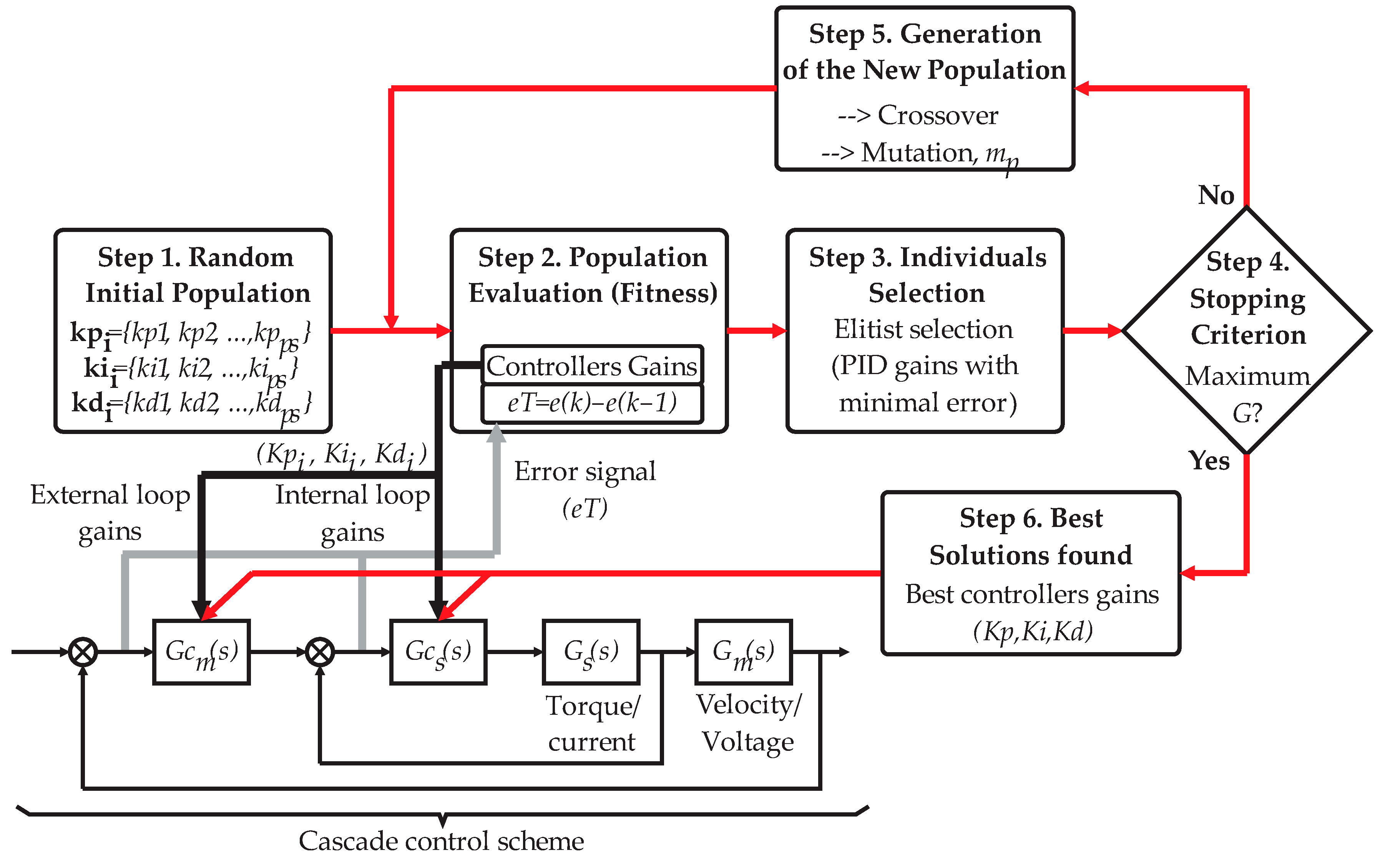
  • Step 1: Randomly generate an initial population. Every individual represents the three gains of a PID regulator (Proportional k p i , Integral k i i , and Derivative k d i ). Where i = 1, 2, 3, …, and p s is the i-th gain of an individual from a total of p s individuals in the population. The length of the string representation per individual is t s l , each gain’s string length is specified in a fixed-point format, the searching ranges of the gains are given according to the fixed-point format, and initial values (seed values) are given through the tuning rules of Ziegler–Nichols (ZN), see Table 2. Thus, the random population is generated around the seed values.
  • Step 2: Evaluate the population’s fitness. The gains of every individual in the population are set on the PIDs of the corresponding cascade control scheme (Torque–Velocity or Voltage–Current), and their response performances are analyzed. For example, the error signals generated in the cascade scheme are stored in the global variable e T , which are the feedback to this sub block, and they are used in the objective function trying to minimize the error e k with respect to its previous value e ( k 1 ) . From the cascade control scheme of Figure 7, G s ( s ) represents the secondary process with the fast variable (Torque/Current); G m ( s ) represents the main process with the slow variable (Velocity/Voltage); and G c s ( s ) and G c m ( s ) are the corresponding PID controller algorithms.
  • Step 3: Perform the selection of individuals according to their fitness values, which means that the individuals (controller gains) with the best performances will be sorted in descending order. The controller gains in upper positions are selected (elitist selection).
  • Step 4: Evaluate the stopping criterion. It is based on the maximum number of generations G . If satisfied, then go to Step 6; if not, then go to Step 5.
  • Step 5: Generate a new population. The initial population will be substituted by a new population created through the genetic operator’s crossover and mutation. The crossover operation is performed considering one crossover point. By its part, the mutation is applied considering one mutation bit having the mutation probability m p , with the purpose of avoiding losing essential genetic information. Then, go to Step 2.
  • Step 6: The best solutions found are set as the gains of the controllers G c s ( s ) and G c m ( s ) in the cascade scheme.
As it can be noted from Figure 7, this heuristic approach is applied in both cascade control schemes.

3. Results and Discussion

3.1. Experimental Setup

The experimental setup for testing the proposed HIL structure is described in this subsection. A PC laptop with the Windows 10 operating system having the following hardware features was used for running the simulation environment. A total of 32 gigabytes (GB) of integrated random-access memory (RAM) running at 1666 megahertz (MHz) was used. The device processor was an Intel Core i7-8750H operating at a frequency of 2.2 gigahertz (GHz). Additionally, a dedicated graphics video card model NVIDIA GeForce GTX 1060 was used for running the simulations. In relation to the software used for implementing the hardware-in-the-loop structure for testing the linear cascade control schemes tuned by the GA applied on a BLDC motor used in a two-wheeler electric scooter, Typhoon HIL Schematic Editor version 2021.3 (×64) was used. The features considered for the BLDC motor were those summarized in Table 1.
Table 3 presents the matrix of experimentations that were carried out on the proposed HIL under different operating conditions. From table five, case studies are observed considering changes in the wind speed (CE1), changes in the slope angle theta (CE2), and combined changes, including the system’s mass, in the operating conditions (CE3, CE4, and CE5). Therefore, the first column of the table indicates the trial identifier; the columns 2, 3, and 4 are the parameter values of the operating conditions (MASS, WS, Theta); and the changes in the values can be observed for a same case study. Finally, the fourth column indicates the moment in which the parameter variation is made, expressed in seconds.
In addition, it is worth mentioning that the GA-PID Tuner operates iteratively during the HIL simulation; thus, the gains of the controllers in the cascade schemes are not constant, but they are adaptively adjusted. Therefore, for illustrative purposes, only an example of the gain’s optimization for the CE5 is displayed through the plots of Figure 8. This way, Figure 8a displays the variation in the controller gains for the cascade scheme Voltage–Current, whereas Figure 8b shows the adjustment of the controller gains for the cascade scheme Speed–Torque.

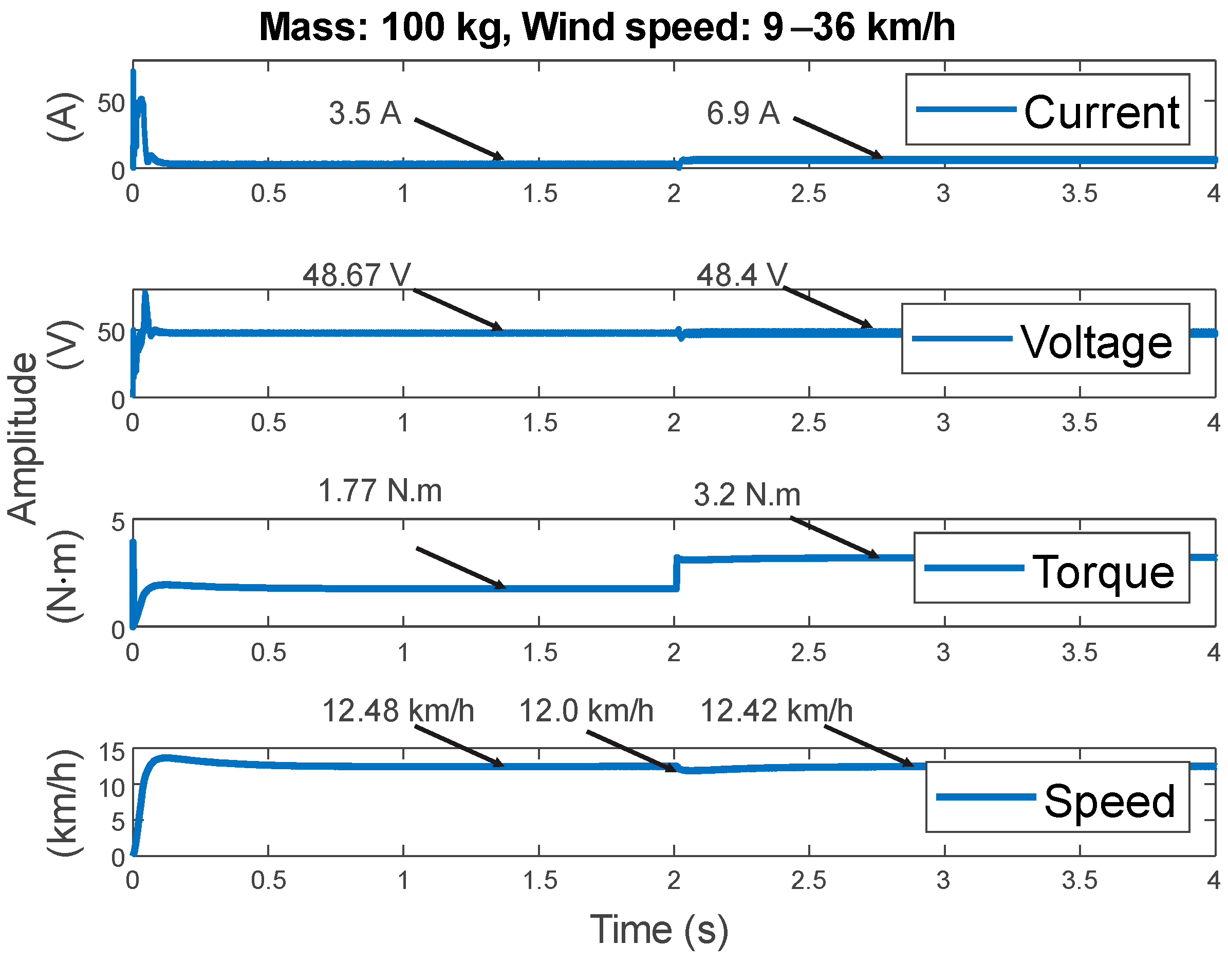
3.2. Results Obtained for the CE1

The first case study was defined for testing the proposed HIL and the linear cascade control schemes under changes in the operating conditions related to the force generated by variations in the system aerodynamics. As explained above, the effective contact area to the wind was mainly related to the user’s and electric scooter’s dimensions; thus, the wind speed would cause a resistance force during the vehicle’s displacement, affecting the current and voltage generated by the bidirectional converter and affecting the reference velocity and required torque. According to Table 3, in this case, the system’s mass was kept constant at a value of 100 k g , there was no slope in the vehicle path (θ = 0°), and the wind speed was the variable parameter. Therefore, the electric scooter started its travel considering a wind speed against it of 9 k m / h , but this speed suddenly changed to a value of 36 k m / h after 2 s. The results obtained in applying the linear controllers in a cascade scheme are displayed in the plots of Figure 9.
From Figure 9, four plots arranged in rows can be noted. The first plot is the current provided by the bidirectional converter and demanded by the BLDC motor; the second plot, similarly, is the voltage provided by the converter to the motor; the third plot is the torque generated by the motor; and the fourth plot is the velocity reached by the scooter. It is worth mentioning that these variables (current and voltage of the bidirectional converter, torque and velocity of the BLDC motor) were of interest for all the posterior case studies, and only the parameters associated with the operating conditions would vary. Now, by analyzing the four plots in detail, the affectations in every variable due to the changes in the wind speed being slight, at a time instant of 2 s. In first place, the current graph presents an initial nominal value of 3.5 A , a small disturbance that is quickly compensated for and vanished thanks to the controller, and a slight increment with a value of 6.9 A . It must be noted that the current value must not necessarily have to return to its original level because the increase in the wind speed causes a resistance force that will be reflected by an increment in the demanded current of the motor. In contrast, the voltage graph has an initial value of 48.67 V ; it also presents the same power disturbance vanished by the controller, but, in this case, the voltage remains approximately in the same level of 48.4 V . Regarding the torque graph, it has a nominal initial value of 1.77 N · m , then an increment to a value of 3.2 N · m is observed. This increment is because the motor requires more power to overcome the resistance force caused by the wind. Last but not least, the velocity of the electric scooter starts with a nominal value of 12.48 k m / h , then it is slightly reduced by this resistance force to 12.0 k m / h , but the controller allows the system to reach the value of 12.42 k m / h a half second later.

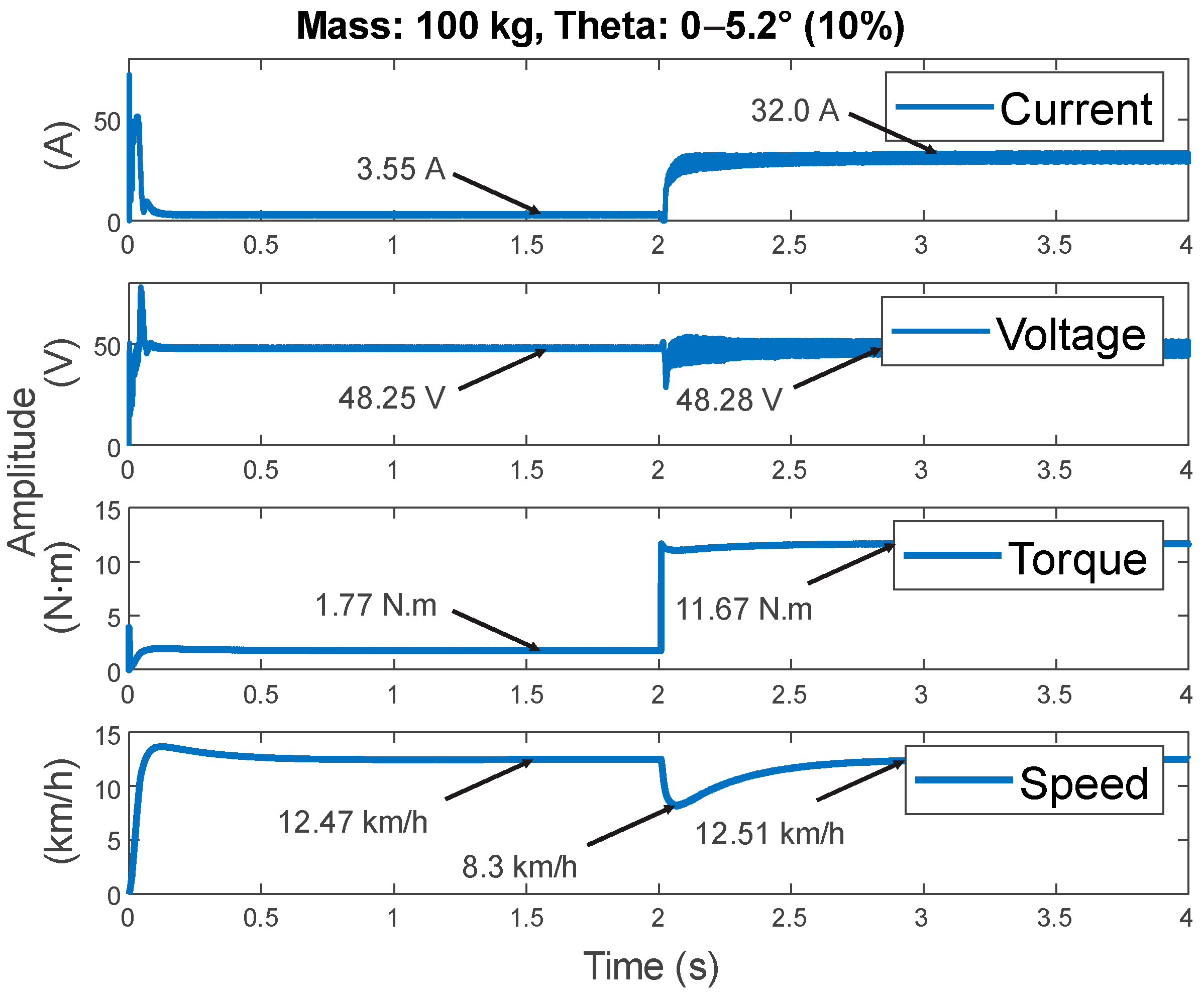
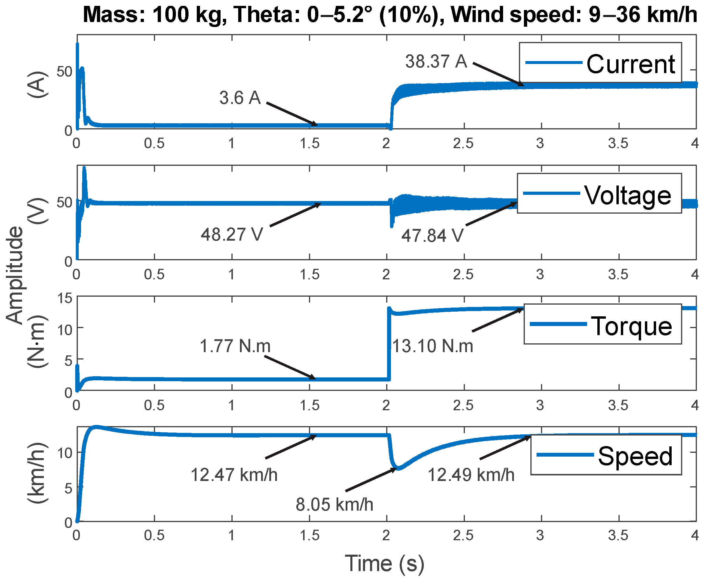
3.3. Results Obtained for the CE2

In the second case study, the proposed HIL and the linear cascade control schemes were tested for the operating conditions related to the force against the vehicle displacement due to variations on the path slope angle. As in the previous case, the slope angle theta would cause affectations in the variables of the current, voltage, velocity, and torque during the vehicle displacement. From Table 3, in this case, the system mass was kept constant at a value of 100 k g , the wind speed remained constant with a value of 9 k m / h , and the slope angle theta in the vehicle path was the variable parameter. Therefore, the electric scooter started its travel on a flat path, but, after 2 s, a slope with an inclination angle of 5.2° appeared. The results obtained of applying the linear controllers in a cascade scheme are displayed in the plots of Figure 10.
From Figure 10, the four plots, arranged in rows, represent the same variables as the previous case. Therefore, by analyzing the four plots in detail, the affectations in every variable due to the change on the path slope angle at instant time of 2 s are notorious. Here, the current graph starts with a nominal current of 3.55 A , then a major disturbance that is quickly compensated for by the controller is observed, and also a big increment in the current level of the converter of 32.0 A is observed. This new level of the current demanded by the motor is necessary to guarantee the motor’s operation during the electric scooter’s displacement on the slope. By its part, the voltage graph begins with a nominal voltage of 48.25 V , then the power disturbance is minimized by the controller and keeps the voltage level at 48.28 V . The torque graph reflects a big increment from approximately 1.77 N · m to a value of 11.67 N · m because the motor will require this new level of power to go up on this slope angle in the path. Finally, the velocity of the electric scooter is reduced from 12.47 k m / h to a value of 8.3 k m / h due to the slope, but the controller achieves that the vehicle reaches 12.51 k m / h almost one second later.

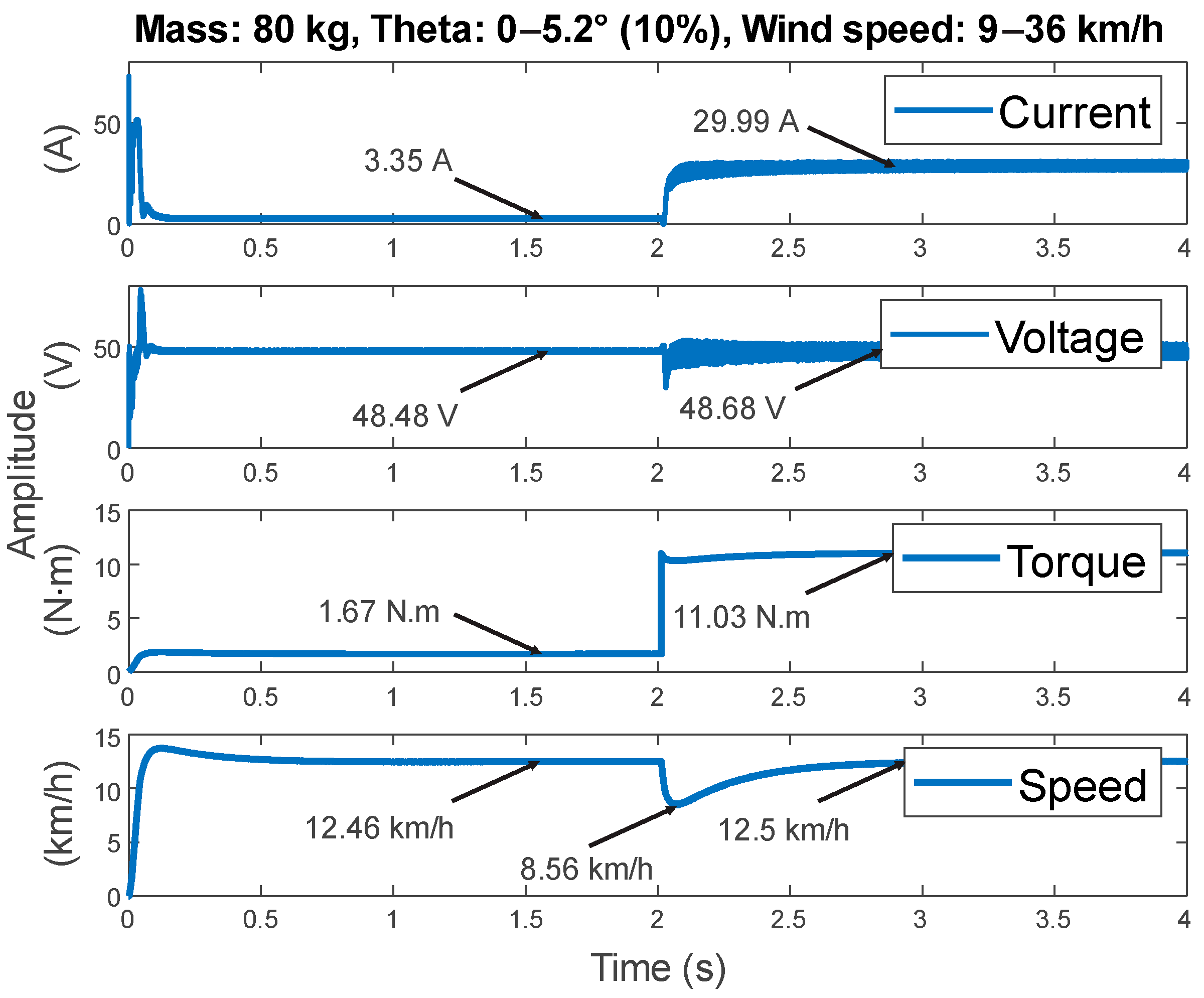
3.4. Results Obtained for the CE3

In the third case study, the operating conditions were analyzed for the proposed HIL, and the linear cascade control schemes were the combinations of the parameters related with the external forces. In this case, the affectations of current, voltage, velocity, and torque during the vehicle’s displacement would be caused by the resistance force because of the wind, a slope in the path, and a reduction in mass. Now, according to Table 3, the system mass was reduced to a constant value of 80 k g . Meanwhile, the wind speed and the slope angle theta were variable parameters. This way, the electric scooter started its travel in a flat path, with an initial velocity of 9 k m / h , but a slope with an inclination angle of 5.2° appeared after 2 s, and the velocity increased suddenly to a value of 36 k m / h . The results obtained of applying the linear controllers in a cascade scheme are displayed in the plots of Figure 11.
Figure 11 presents the corresponding plots of current, voltage, torque, and speed, arranged in rows, for the electric scooter. Through a deep analysis of the four figures, it can be noted the disturbance caused by the operating conditions changed at the 2 s time point, which was notorious, and some variables increased their magnitude. Hence, the graph of current presented an increment from 3.35 A to 29.99 A , and this new level of the current demanded by the motor was necessary to guarantee the motor’s operation during the electric scooter’s displacement on the slope. By its part, the voltage graph presented a disturbance that the controller tried to vanish to maintain the voltage at around 48.68 V from its original value of 48.48 V . The torque graph reflected a significative increment from 1.67 N · m to a value of 11.03 N · m because the motor would require this new level of power to go up through this slope angle in the path. Finally, the velocity of the electric scooter was reduced from approximately 12.46 km/h to a value of 8.56 km/h due to the slope, but the controller achieved that the vehicle reached 12.5 k m / h almost one second later.

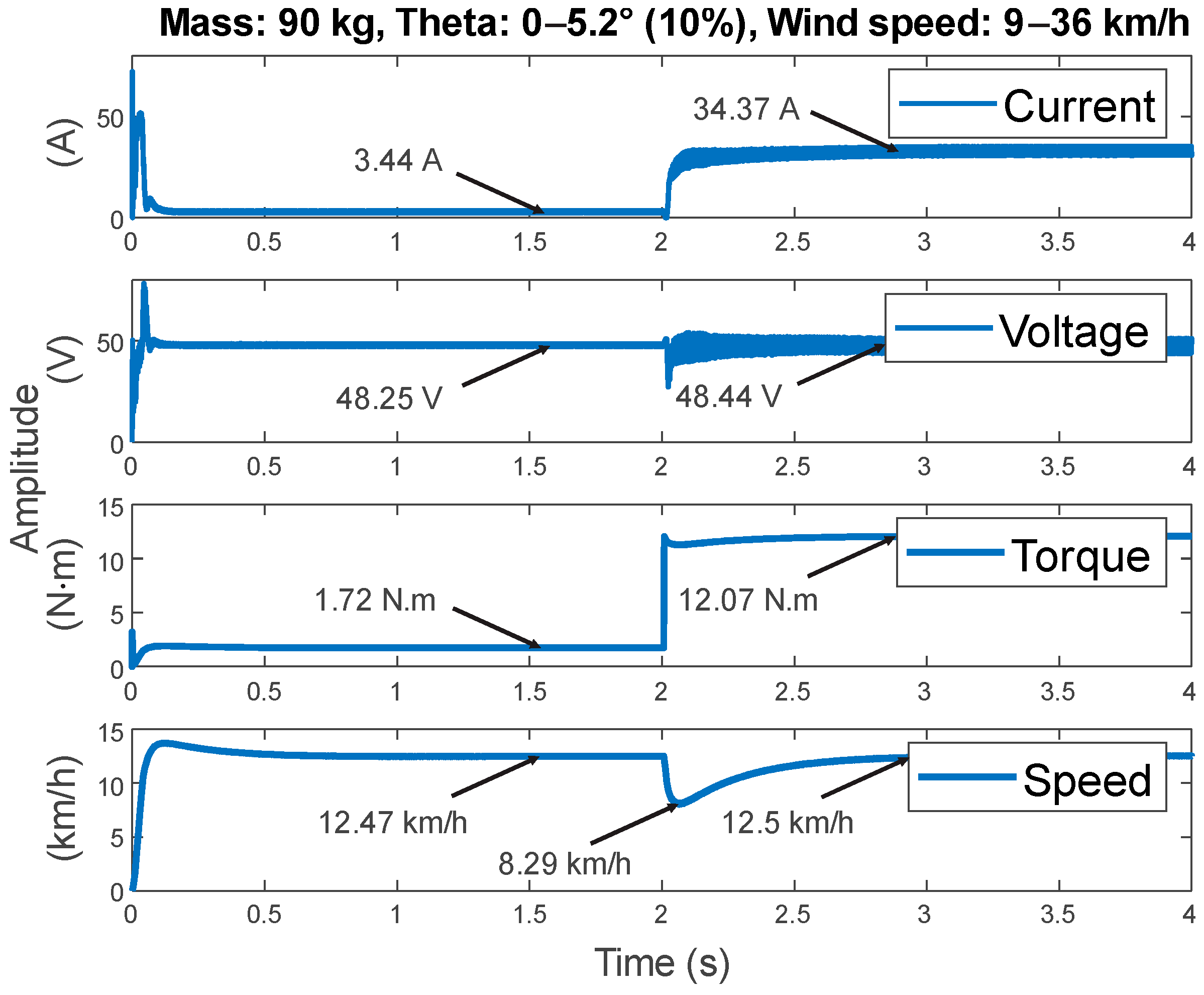
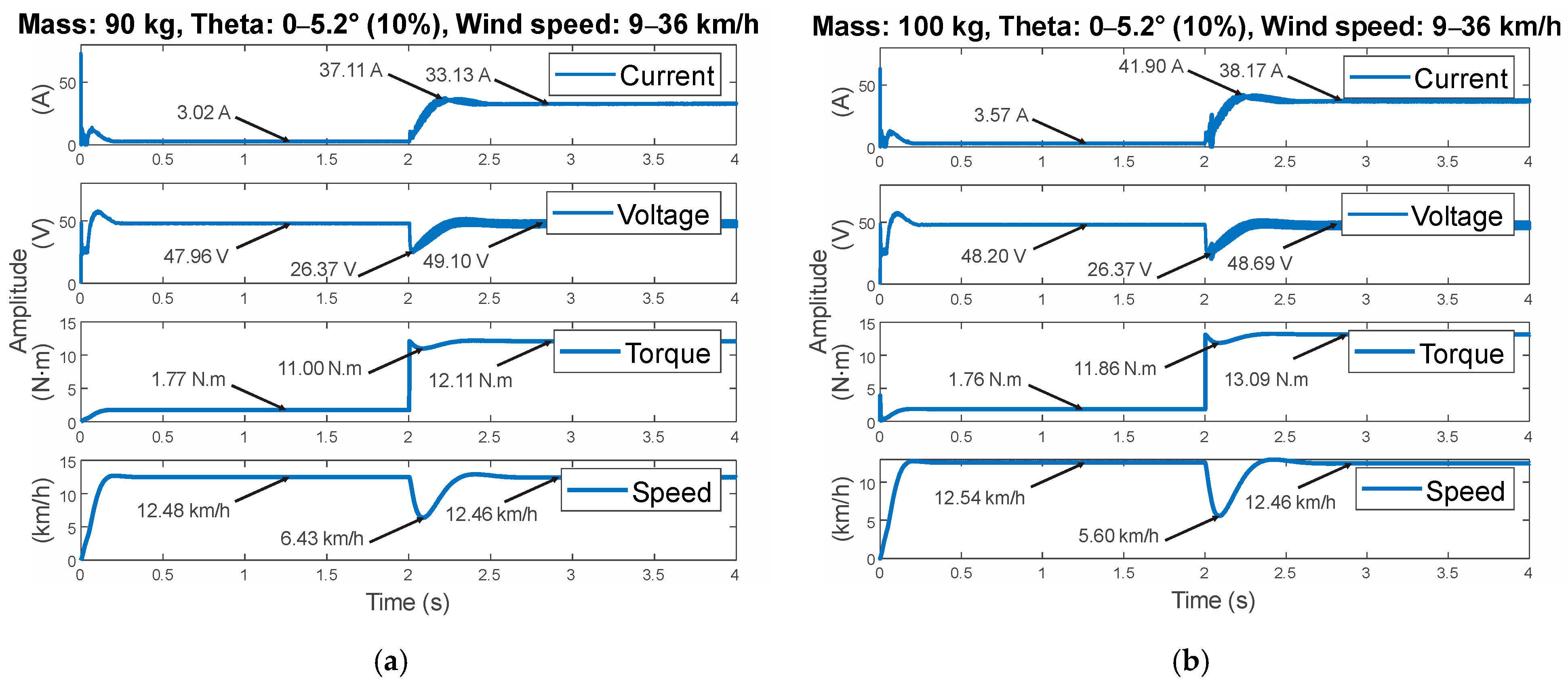
3.5. Results Obtained for the CE4

In the fourth case study, similar to the previous case, the affectations in current, voltage, velocity, and torque during the vehicle displacement would be caused by the resistance force because of the wind, a slope in the path, and a reduction in mass. According to Table 3, the system mass increased by 10 k g with respect to the previous case, leaving a constant value of 90 k g . The wind speed and the slope angle theta were still variable parameters. Thus, the electric scooter started its travel in a flat path with an initial velocity of 9 k m / h , but a slope with an inclination angle of 5.2° appeared after 2 s, and the velocity increased suddenly to a value of 36 k m / h . The results obtained in applying the linear controllers in a cascade scheme are displayed in the plots of Figure 12.
Figure 12 presents the corresponding plots of current, voltage, torque, and speed. As in the previous cases, the disturbance was notoriously observed at 2 s. In this case, the graph of current changed from 3.44 A to 34.37 A . By its part, the voltage graph presented a disturbance vanished by the controller that also maintained the voltage around 48.44 V from its original value of 48.25 V . The torque graph presented an increment from 1.72 N · m to a value of 12.07 N · m . Finally, the velocity of the electric scooter was reduced from approximately 12.47 km/h to a value of 8.29 km/h, but the controller ensured that the vehicle reached 12.5 k m / h almost one second later.

3.6. Results Obtained for the CE5

In the fifth case study, similarly as the previous case, and according to Table 3, the system mass is newly increased 10 k g with respect to the previous case, leaving a constant value of 100 k g . The wind speed and the slope angle theta are still variable parameters. Therefore, the electric scooter starts its travel in a flat path with an initial velocity of 9 k m / h , but after 2 s a slope with an inclination angle of 5.2° appears and the velocity increases suddenly to a value of 36 k m / h . The results obtained of applying the linear controllers in a cascade scheme are displayed in the plots of Figure 13.
From Figure 13, the graph of current changes from 3.6 A to 38.37 A . The voltage graph presents a disturbance vanished by the controller that also maintains the voltage around 47.84 V form its original value of 48.27 V . The torque graph presents an increment from 1.77 N · m to a value of 13.10 N · m . Finally, the velocity of the electric scooter is reduced from approximately 12.47 km/h to a value of 8.05 km/h, but the controller achieves that the vehicle reaches 12.49 k m / h almost one second later.
In summary, from Figure 11, Figure 12 and Figure 13, the system’s behavior was very similar between these plots. However, as the system’s mass was changed between these cases by 10 k g of difference in each one, proportional changes were observed in the analyzed variables as a consequence. For instance, the currents’ and torques’ ranges were increased in accordance to the system’s mass increases, but also the electric scooter’s velocity was reduced proportionally as well. Only the voltage behaved very similar for these last three cases. Now, regarding the controllers in the cascade schemes’ performance, it can be said that the two variables that needed to be guaranteed were accomplished, such as the case of the voltage level that was kept around 48 V and the vehicle speed that was kept around the specified reference at 12.0 k m / h . For the variables of current and torque, these were incremented according to the system’s demand, with the purpose of compensating for the operating condition variation.

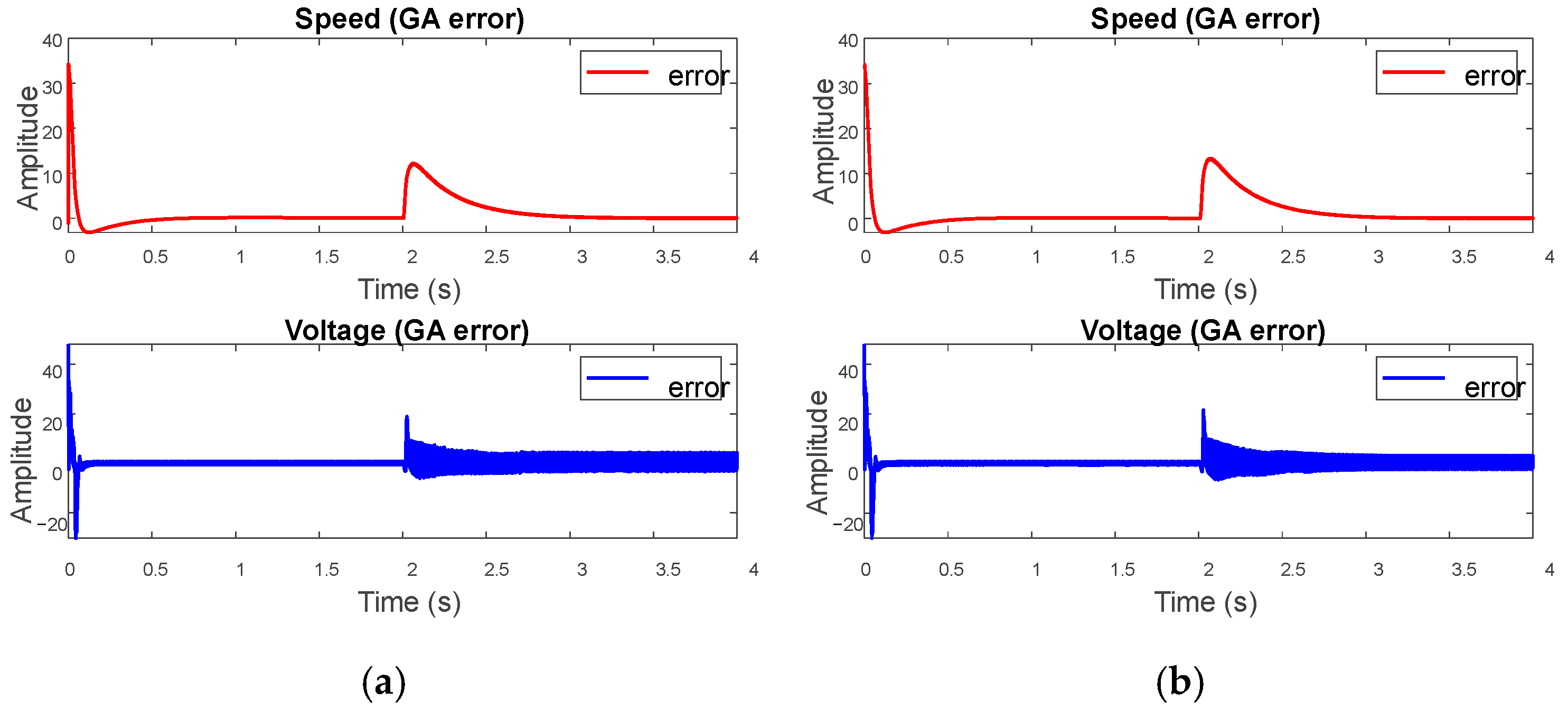
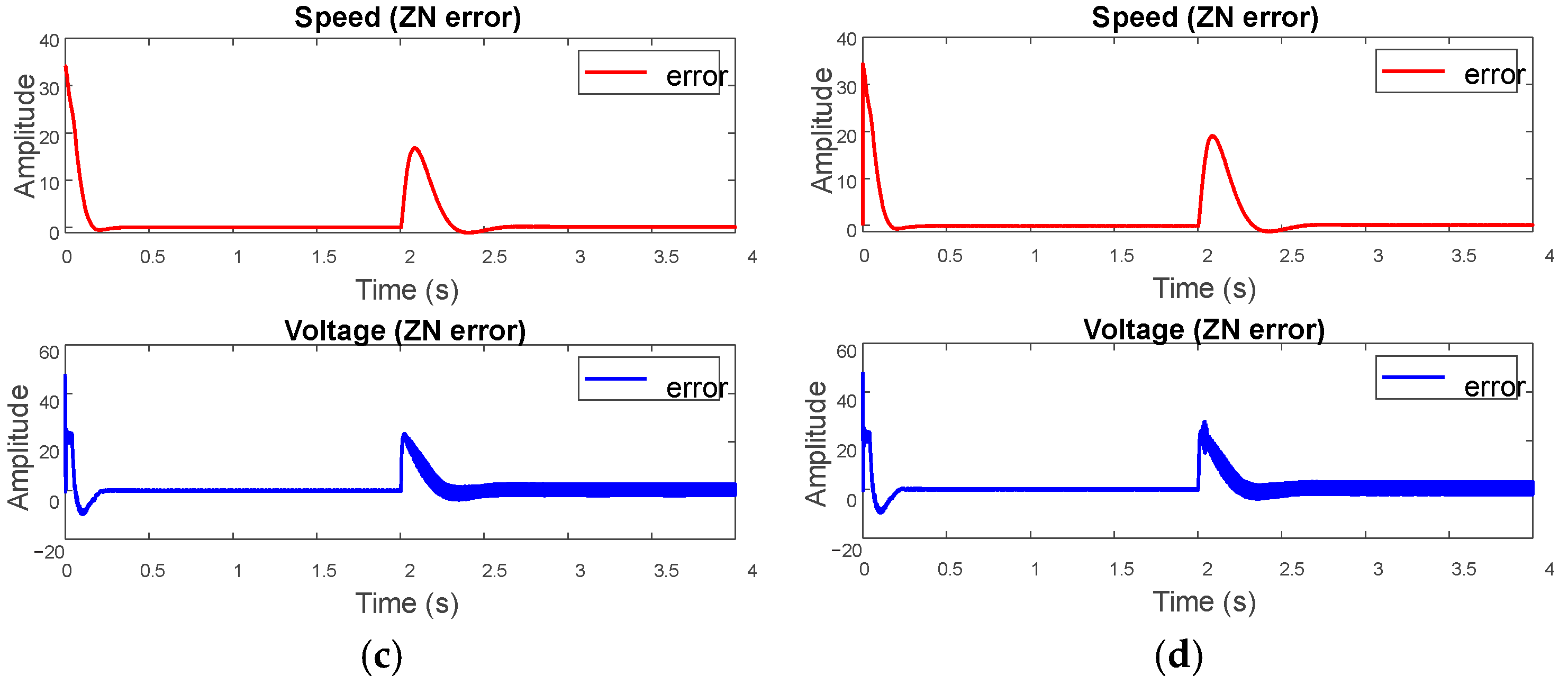
3.7. Comparison with a Classical PID Control Tuned through ZN, CE4, and CE5

For comparative purposes with a classical control, the results of the PID controllers tuned through the rules of Ziegler–Nichols (ZN) were included as an example of the advantages of this proposal, and only the corresponding case studies CE4 and CE5 were considered for this comparison. The plots of Figure 14 depict the model responses when the control scheme was not optimized through the GA technique, and the gains were not adaptively being adjusted, but, instead, the gains were obtained through the ZN rules. This way, Figure 14a shows the response of the cascade control schemes for the CE4, the graphs of current, voltage, torque, and speed appearing in descending order. Similarly, Figure 14b shows the corresponding graphs for the CE5.
From these graphs, significant variations in the response signals of every variable can be observed, and, for that reason, the values of these points of interest are shown, indicating bigger changes than those results obtained through GA for the same case. For example, in the time instant t = 2 s in both set of plots, the numerical values pointed with arrows show greater overshoots in the current signals (31.11 A and 41.90 A for the CE4 and CE5, respectively) in contrast with their analogous response obtained from the GA (which are very slight). By its part at the same time instant, the numerical values pointed with arrows show greater signal drops for the speed variables (6.43 km/h and 5.6 km/h for the CE4 and CE5, respectively) than their counterpart plots obtained by using the GA. A similar analysis can be developed for the voltage and torque variables.
Next, the following plots of Figure 15 show the error signals generated in the external loops of the cascade control schemes. For instance, the speed error is the difference between the speed reference and the real speed reached by the electrical scooter through the cascade Speed–Torque scheme. Meanwhile, the voltage error is the difference between the voltage reference (48 VDC) and the real voltage ensured at the bidirectional buck-boost converter through the cascade Voltage–Current scheme.
Figure 15a,b show the plots of the error signals corresponding to the speed and the voltage variables for the CE4 and CE5, respectively, when the cascade control schemes are tuned through the GA. Meantime, Figure 15c,d present the graphs of the error signals for the same two variables and for the same case studies, but when the cascade control scheme is tuned through the ZN rules. By observing the error plots in the time instant t = 2 s during a reference change, it can be noted that the graphs obtained through the GA had lower peak amplitudes than their counterpart ZN values in all cases. However, additionally, the plots of voltage errors obtained from the ZN rules took longer times to remove the effects of the reference changes than their analogous results by using the GA. The reasons for why only the speed and voltage variables were displayed without considering the internal loops of the cascade schemes were because the references for the torque and current signals were dependent on the outputs of the external loop controllers. Thus, these signals would not have intuitive variations since the final speed reached by the scooter depended on the torque demanded, and the current demanded from the bidirectional buck-boost converter still required keeping the voltage constant.
Finally, with the objective of providing a quantitative performance analysis, a numerical representation of the plots of Figure 15 is presented through the values of Table 4. The mean square error (MSE) is the feature considered for the analysis. It is obtained from the error signals generated by using the GA and those signals generated by using the ZN. It can be observed with more clarity that the MSE values are lower for the speed and voltage when the tuning process of the cascade control schemes is performed by the GA PID Tuner. In fact, the relative response improvements in reducing the MSE, with the cascade control schemes tuned by using the GA with respect to the classical tuning through the ZN rules, are of 20.53% for the speed and 52.02% for the voltage, respectively, in the CE4. On the other hand, the corresponding relative response improvements (GA Vs ZN) are of 31.72% for the speed and 63.70% for the voltage, respectively, in the CE5.

4. Conclusions

This paper presented the development and implementation of a hardware-in-the-loop (HIL) simulation focused on cascade linear PID controllers, tuned by genetic algorithms (GAs), applied to the BLDC motor used in a two-wheeler electric scooter. The proposed HIL platform allowed us to develop a fast and secure design of physical systems without the need to have the real system and, of course, without compromising the physical system’s integrity. On the other hand, in the proposed HIL, two cascade PID controllers were implemented and applied in two subsystems of the electric scooter, which were the bidirectional converter and the BLDC motor. These controllers were designed with the purpose of guaranteeing the electric scooter requirements for its proper operation, similar to the electrical source that provided demanded current and a constant voltage or in the power inverter for maintaining a constant speed with changes in torque. From the results, it could be concluded that the controllers had good performances since the voltage of the converter and the reference velocity of the scooter were regulated around their references (48 V and 12 k m / h ). Even considering that operating conditions were changed through parameters such as mass, wind speed, and slope angle, affecting the system’s behavior, the controllers worked very well, and it could be achieved because of the controller gain optimizations through the heuristic tuning based on the GA. In future work, other aspects of this type of electric vehicle will be addressed, such as the part of energy recovery through regenerative braking. Additionally, additional operating conditions could be added to the proposed model, such as sudden braking or emergency stops, path rugosity, etc.

Author Contributions

Conceptualization, R.A.O.-R. and L.M.-V.; methodology, R.A.O.-R. and L.M.-V.; software, L.E.M.-S.; validation, L.E.M.-S., A.Y.J.-C. and L.M.-V.; formal analysis, L.E.M.-S. and A.Y.J.-C.; investigation, A.Y.J.-C.; resources, L.E.M.-S.; data curation, L.E.M.-S. and L.M.-V.; writing—original draft preparation, A.Y.J.-C.; writing—review and editing, A.Y.J.-C.; visualization, A.Y.J.-C.; supervision, R.A.O.-R.; project administration, R.A.O.-R.; funding acquisition, R.A.O.-R. All authors have read and agreed to the published version of the manuscript.

Funding

This research received no external funding.

Data Availability Statement

Data sharing not applicable.

Acknowledgments

CONACyT scholarship number 931510.

Conflicts of Interest

The authors declare no conflict of interest.

References

  1. Coretti Sanchez, N.; Martinez, I.; Alonso Pastor, L.; Larson, K. On the Simulation of Shared Autonomous Micro-Mobility. Commun. Transp. Res. 2022, 2, 100065. [Google Scholar] [CrossRef]
  2. Bharathidasan, M.; Indragandhi, V.; Suresh, V.; Jasiński, M.; Leonowicz, Z. A Review on Electric Vehicle: Technologies, Energy Trading, and Cyber Security. Energy Rep. 2022, 8, 9662–9685. [Google Scholar] [CrossRef]
  3. Zhang, H.; Chen, D.; Zhang, H.; Liu, Y. Research on the Influence Factors of Brake Regenerative Energy of Pure Electric Vehicles Based on the CLTC. Energy Rep. 2022, 8, 85–93. [Google Scholar] [CrossRef]
  4. Olabi, A.G.; Wilberforce, T.; Obaideen, K.; Sayed, E.T.; Shehata, N.; Alami, A.H.; Abdelkareem, M.A. Micromobility: Progress, Benefits, Challenges, Policy and Regulations, Energy Sources and Storage, and Its Role in Achieving Sustainable Development Goals. Int. J. 2023, 17, 100292. [Google Scholar] [CrossRef]
  5. Sandt, L. The Basics of Micromobility and Related Motorized Devices for Personal Transport. Pedestrian and Bicycle Information Center. 2019. Available online: http://pedbikeinfo.org/cms/downloads/PBIC_Brief_MicromobilityTypology.pdf (accessed on 1 May 2023).
  6. Comi, A.; Polimeni, A.; Nuzzolo, A. An Innovative Methodology for Micro-Mobility Network Planning. Transp. Res. Procedia 2022, 60, 20–27. [Google Scholar] [CrossRef]
  7. Samadzad, M.; Nosratzadeh, H.; Karami, H.; Karami, A. What Are the Factors Affecting the Adoption and Use of Electric Scooter Sharing Systems from the End User’s Perspective? Transp. Policy 2023, 136, 70–82. [Google Scholar] [CrossRef]
  8. Indragandhi, V.; Subramaniyaswamy, V.; Selvamathi, R. Chapter 8—Electric Drives Used in Electric Vehicle Applications. In Electric Motor Drives and Their Applications with Simulation Practices; Indragandhi, V., Subramaniyaswamy, V., Selvamathi, R., Eds.; Academic Press: Cambridge, MA, USA, 2022; pp. 435–479. ISBN 978-0-323-91162-7. [Google Scholar]
  9. Lee, K.-J.; Yun, C.H.; Yun, M.H. Contextual Risk Factors in the Use of Electric Kick Scooters: An Episode Sampling Inquiry. Saf. Sci. 2021, 139, 105233. [Google Scholar] [CrossRef]
  10. van Boven, J.F.M.; An, P.L.; Kirenga, B.J.; Chavannes, N.H. Electric Scooters: Batteries in the Battle against Ambient Air Pollution? Lancet Planet. Health 2017, 1, e168–e169. [Google Scholar] [CrossRef]
  11. Chou, J.-R.; Hsiao, S.-W. Product Design and Prototype Making for an Electric Scooter. Mater. Des. 2005, 26, 439–449. [Google Scholar] [CrossRef]
  12. Falai, A.; Giuliacci, T.A.; Misul, D.; Paolieri, G.; Anselma, P.G. Modeling and On-Road Testing of an Electric Two-Wheeler towards Range Prediction and BMS Integration. Energies 2022, 15, 2431. [Google Scholar] [CrossRef]
  13. Magibalan, S.; Ragu, C.; Nithish, D.; Raveeshankar, C.; Sabarish, V. Design and Fabrication of Electric Three-Wheeled Scooter for Disabled Persons. Mater. Today Proc. 2023, 74, 820–823. [Google Scholar] [CrossRef]
  14. Yu, M.; Xiao, C.; Wang, H.; Jiang, W.; Zhu, R. Adaptive Cuckoo Search-Extreme Learning Machine Based Prognosis for Electric Scooter System under Intermittent Fault. Actuators 2021, 10, 283. [Google Scholar] [CrossRef]
  15. Kalyankar-Narwade, S.; Chidambaram, R.K.; Patil, S. Neural Network- and Fuzzy Control-Based Energy Optimization for the Switching in Parallel Hybrid Two-Wheeler. World Electr. Veh. J. 2021, 12, 35. [Google Scholar] [CrossRef]
  16. Sandesh, B.B.; Jogi, A.; Pitchaimani, J.; Gangadharan, K.V. Design and Optimization of an External-Rotor Switched Reluctance Motor for an Electric Scooter. Mater. Today Proc. 2023, 1–6. [Google Scholar] [CrossRef]
  17. Burbank, J.L.; Kasch, W.; Ward, J. Hardware-in-the-Loop Simulations. In An Introduction to Network Modeling and Simulation for the Practicing Engineer; Wiley-IEEE Press: Cambridge, MA, USA, 2011; pp. 114–142. ISBN 978-1-118-06365-1. [Google Scholar]
  18. Lee, J.S.; Choi, G. Modeling and Hardware-in-the-Loop System Realization of Electric Machine Drives—A Review. CES Trans. Electr. Mach. Syst. 2021, 5, 194–201. [Google Scholar] [CrossRef]
  19. Abu-Rub, H.; Malinowski, M.; Al-Haddad, K. Hardware-in-the-Loop Systems with Power Electronics: A Powerful Simulation Tool. In Power Electronics for Renewable Energy Systems, Transportation and Industrial Applications; Wiley-IEEE Press: Manhattan, NY, USA, 2014; pp. 573–590. ISBN 978-1-118-75552-5. [Google Scholar]
  20. Sparn, B.; Krishnamurthy, D.; Pratt, A.; Ruth, M.; Wu, H. Hardware-in-the-Loop (HIL) Simulations for Smart Grid Impact Studies. In Proceedings of the 2018 IEEE Power & Energy Society General Meeting (PESGM), Portland, OR, USA, 5–10 August 2018; pp. 1–5. [Google Scholar]
  21. Tsampardoukas, G.; Mouzakitis, A. Hardware-in-the-Loop Visual Display Validation Utilising Vision System. In Proceedings of the UKACC International Conference on Control 2010, Coventry, UK, 7–10 September 2010; pp. 1–5. [Google Scholar]
  22. Joshi, A. Automotive Applications of Hardware-in-the-Loop (HIL) Simulation. In Automotive Applications of Hardware-in-the-Loop (HIL) Simulation; SAE: Warrendale, PA, USA, 2020; pp. i–xxvii. ISBN 978-1-4686-0007-0. [Google Scholar]
  23. Essa, M.E.-S.M.; Lotfy, J.V.W.; Abd-Elwahed, M.E.K.; Rabie, K.; ElHalawany, B.M.; Elsisi, M. Low-Cost Hardware in the Loop for Intelligent Neural Predictive Control of Hybrid Electric Vehicle. Electronics 2023, 12, 971. [Google Scholar] [CrossRef]
  24. Gros, I.-C.; Fodorean, D.; Marginean, I.-C. FPGA Real-Time Implementation of a Vector Control Scheme for a PMSM Used to Propel an Electric Scooter. In Proceedings of the 2017 5th International Symposium on Electrical and Electronics Engineering (ISEEE), Galati, Romania, 20–22 October 2017; pp. 1–5. [Google Scholar]
  25. Wu, C.-H.; Hung, Y.-H.; Chen, S.-Y. Rapid-Prototyping Designs for the Three-Power-Source Hybrid Electric Scooter with a Fuzzy-Control Energy Management. In Proceedings of the 2016 International Conference on Applied System Innovation (ICASI), Okinawa, Japan, 26–30 May 2016; pp. 1–4. [Google Scholar]
  26. Mohanraj, D.; Aruldavid, R.; Verma, R.; Sathiyasekar, K.; Barnawi, A.B.; Chokkalingam, B.; Mihet-Popa, L. A Review of BLDC Motor: State of Art, Advanced Control Techniques, and Applications. IEEE Access 2022, 10, 54833–54869. [Google Scholar] [CrossRef]
  27. Riyadi, S.; Dwi Setianto, Y.B. Analysis and Design of BLDC Motor Control in Regenerative Braking. In Proceedings of the 2019 International Symposium on Electrical and Electronics Engineering (ISEE), Ho Chi Minh City, Vietnam, 10–12 October 2019; pp. 211–215. [Google Scholar]
  28. Mamadapur, A.; Unde Mahadev, G. Speed Control of BLDC Motor Using Neural Network Controller and PID Controller. In Proceedings of the 2019 2nd International Conference on Power and Embedded Drive Control (ICPEDC), Chennai, India, 21–23 August 2019; pp. 146–151. [Google Scholar]
  29. Ibrahim, M.A.; Mahmood, A.K.; Sultan, N.S. Optimal PID Controller of a Brushless Dc Motor Using Genetic Algorithm. Int. J. Power Electron. Drive Syst. IJPEDS 2019, 10, 822–830. [Google Scholar] [CrossRef] [Green Version]
  30. Hicham, C.; Nasri, A.; Kayisli, K. A Novel Method of Electric Scooter Torque Estimation Using the Space Vector Modulation Control. Int. J. Renew. Energy Dev. 2021, 10, 355–364. [Google Scholar] [CrossRef]
  31. Jorge, I.; Mesbahi, T.; Paul, T.; Samet, A. Study and Simulation of an Electric Scooter Based on a Dynamic Modelling Approach. In Proceedings of the 2020 Fifteenth International Conference on Ecological Vehicles and Renewable Energies (EVER), Monte-Carlo, Monaco, 10–12 September 2020; pp. 1–6. [Google Scholar]
  32. Kumar, K.V.; Voora, S.; Raghavender, A.T. Genetic Algorithm and Its Applications to Mechanical Engineering: A Review. Mater. Today Proc. 2015, 2, 2624–2630. [Google Scholar] [CrossRef]
Figure 1. General block diagram of two-wheeler electrical scooter, subsystems, and operating conditions considered.
Machines 11 00663 g001
Figure 2. Free-body diagram of the external forces affecting the two-wheeler electric scooter’s displacement.
Machines 11 00663 g002
Figure 3. Complete structure of the proposed HIL system for the linear controllers, tuned by the GA, applied to the two-wheeler electric scooter BLCD motor.
Machines 11 00663 g003
Figure 4. Operating conditions subsystem into the HIL structure.
Machines 11 00663 g004
Figure 5. Converter controller subsystem into the HIL structure.
Machines 11 00663 g005
Figure 6. BLDC controller subsystem into the HIL structure.
Machines 11 00663 g006
Figure 7. GA PID Tuner block diagram.
Machines 11 00663 g007
Figure 8. Plots of the adaptive gains variation through GA PID Tuner into the HIL structure of the CE5, (a) in gains of the cascade control Voltage–Current and (b) in gains of the cascade control Speed–Torque.
Machines 11 00663 g008
Figure 9. Results of the case study CE1 in the HIL simulation, compensation of the linear controllers in a cascade scheme applied to the BLDC motor used in the two-wheeler electric scooter.
Machines 11 00663 g009
Figure 10. Results of the case study CE2 in the HIL simulation, compensation of the linear controllers in a cascade scheme applied to the BLDC motor used in the two-wheeler electric scooter.
Machines 11 00663 g010
Figure 11. Results of the case study CE3 in the HIL simulation, compensation of the linear controllers in a cascade scheme applied to the BLDC motor used in the two-wheeler electric scooter.
Machines 11 00663 g011
Figure 12. Results of the case study CE4 in the HIL simulation, compensation of the linear controllers in a cascade scheme applied to the BLDC motor used in the two-wheeler electric scooter.
Machines 11 00663 g012
Figure 13. Results of the case study CE5 in the HIL simulation, compensation of the linear controllers in a cascade scheme applied to the BLDC motor used in the two-wheeler electric scooter.
Machines 11 00663 g013
Figure 14. Results of the control schemes tuned through the rules of ZN (a) in system responses for the CE4 and (b) in system responses for the CE5.
Machines 11 00663 g014
Figure 15. Error plots from the cascade schemes external loops (for all the cases Speed and Voltage) (a) in error signals reached with the GA approach CE4, (b) in error signals reached with the GA approach CE5, (c) in error signals reached with the classical ZN approach CE4, and (d) in error signals reached with the classical ZN approach CE5.
Machines 11 00663 g015aMachines 11 00663 g015b
Table 1. Parameters of the BLDC motor considered on the two-wheeler electric scooter.
ParameterValueUnits
Voltage, U 48 V D C
Power350 W
Back-electromotive force constant, k e 17.1 V / k r p m
Resistance, R l 387.1205 m Ω
Inductance, L l 0.8646 m H
Poles number15-
Slots number27-
Moment of Inertia, J 18.8776 k g · m 2
Friction constant, B 0.028 N · m · s
Table 2. Hyperparameters considered for the implementation of the GA.
ParameterValue
Generations number, G 100
Population size, p s 20
Mutation probability, m p 0.1 (10%)
Total string length, t s l 64 bits
Crossover operation1 point
Mutation operation1 bit
Controller Gains Searching Range
GainTorqueVelocityVoltageCurrent
Format/RangeInitial
Value
Format/RangeInitial
Value
Format/RangeInitial
Value
Format/RangeInitial
Value
Kp6.14 bits/
[0, 64)
25.58646.16 bits/
[0, 64)
17.47583.17 bits/
[0, 8)
0.0186.18 bits/
[0, 64)
0.018
Ki8.16 bits/
[0, 256)
106.60986.18 bits/
[0, 64)
2.67329.15 bits/
[0, 512)
12.215818.6 bits/
[0, 262,144)
11.9482
Kd1.19 bits/
[0, 2)
0.00231.17 bits/
[0, 2)
0.01004961.19 bits/
[0, 2)
6.6307 × 10−61.15 bits/
[0, 2)
6.7792 × 10⁻⁶
Table 3. Experimental configuration for the operating conditions changes in the experimentations.
Experimental TrialOperating ConditionsTime
System Mass (MASS)Wind Speed (WS) Slope   Angle   ( θ )
CE1100 kg9 km/ht < 2 s
36 km/h t 2 s
CE2100 kg9 km/ht < 2 s
5.2° (10%) t 2 s
CE380 kg9 km/ht < 2 s
36 km/h5.2° t 2 s
CE490 kg9 km/ht < 2 s
36 km/h5.2° t 2 s
CE5100 kg9 km/ht < 2 s
36 km/h5.2° t 2 s
Table 4. Performance comparison between proposed GA-based approach and classical ZN method.
Case StudyMean Square Error (MSE)
Speed GASpeed ZNVoltage GAVoltage ZN
CE43.8914.68982.81134.2736
CE53.77414.97132.79454.5747
Disclaimer/Publisher’s Note: The statements, opinions and data contained in all publications are solely those of the individual author(s) and contributor(s) and not of MDPI and/or the editor(s). MDPI and/or the editor(s) disclaim responsibility for any injury to people or property resulting from any ideas, methods, instructions or products referred to in the content.

