Article

Gearbox Fault Diagnosis Based on Refined Time-Shift Multiscale Reverse Dispersion Entropy and Optimised Support Vector Machine

1
School of Energy and Power Engineering, Nanjing Institute of Technology, Nanjing 211167, China
2
School of Electrical Engineering, Nanjing Institute of Technology, Nanjing 211167, China
*
Author to whom correspondence should be addressed.
Machines 2023, 11(6), 646; https://doi.org/10.3390/machines11060646
Submission received: 19 May 2023 / Revised: 8 June 2023 / Accepted: 9 June 2023 / Published: 13 June 2023
(This article belongs to the Special Issue Vibration Analysis for Structural Health Monitoring)

Abstract

:
The fault diagnosis of a gearbox is crucial to ensure its safe operation. Entropy has become a common tool for measuring the complexity of time series. However, entropy bias may occur when the data are not long enough or the scale becomes larger. This paper proposes a gearbox fault diagnosis method based on Refined Time-Shifted Multiscale Reverse Dispersion Entropy (RTSMRDE), t-distributed Stochastic Neighbour Embedding (t-SNE), and the Sparrow Search Algorithm Support Vector Machine (SSA-SVM). First, the proposed RTSMRDE was used to calculate the multiscale fault features. By incorporating the refined time-shift method into Multiscale Reverse Dispersion Entropy (MRDE), errors that arose during the processing of complex time series could be effectively reduced. Second, the t-SNE algorithm was utilized to extract sensitive features from the multiscale, high-dimensional fault features. Finally, the low-dimensional feature matrix was input into SSA-SVM for fault diagnosis. Two gearbox experiments showed that the diagnostic model proposed in this paper had an accuracy rate of 100%, and the proposed model performed better than other methods in terms of diagnostic performance.

1. Introduction

The gearbox is an important component of mechanical equipment [1]. Continuous work under complex conditions can easily lead to equipment damage [2]. When the gearbox malfunctions, the entire operating equipment will have safety hazards, and the fault signals will exhibit complexity and autocorrelation [3,4]. The implementation of safe and reliable fault diagnosis techniques can effectively prevent serious failures, reduce the operating and maintenance costs, and improve the reliability on mechanical equipment [5].
Due to the highly nonlinear and nonstationary nature of vibration signals from gearbox faults, linear feature extraction methods are not applicable [6]. Therefore, based on nonlinear dynamic theory, entropy methods have been widely used in the detection of rotating machinery dynamic behaviour [7,8]. Entropy, as a parameter for evaluating the regularization process and complexity of time series, is particularly suitable for characterizing nonstationary and nonlinear acceleration signals [9]. Various entropy methods, such as approximate entropy [10], sample entropy [11], fuzzy entropy [12], and permutation entropy [13], have been proposed and used in fault diagnosis. These methods, however, only consider signals at one scale and could ignore crucial temporal information. To overcome this limitation, Costa et al. [14] proposed multiscale entropy. Wang et al. [15] constructed statistical features based on multiscale sample entropy (MSE) to reflect the information of rotating machinery. Zheng et al. [16] combined multiscale fuzzy entropy (MFE) with the SVM to construct an intelligent diagnosis model. Chen et al. [17] combined local mean decomposition and multiscale permutation entropy (MPE) to enhance the feature extraction ability of MPE through pre-processing of the initial signal. These methods have their own deficiencies. Specifically, MSE cannot measure the similarity of short time series, and the calculation of MSE and MFE is very time-consuming for long time series. MPE also ignores the difference between adjacent amplitude values in the time series, which may lead to the neglect of useful information in the amplitude.
Dispersion Entropy (DE) [18] is a new nonlinear dynamic index that overcomes the drawbacks of other entropy algorithms in measuring the complexity and irregularity of time series. When calculating DE, the amplitude of the time series is considered. However, the recognition ability of DE is not very good when dealing with autocorrelated signals. To solve this problem, Azami and Escudero [19] proposed the Dispersion Entropy algorithm based on multiscale fluctuation, which has demonstrated its stability and good recognition ability in processing signals of neurological disorders. Li et al. [20] proposed the reverse dispersion entropy (RDE) algorithm to detect sensor signals and demonstrated its excellent stability through testing with real ship signals. Meanwhile, Xing et al. applied the multiscale method to the RDE algorithm and achieved good results [21]. However, there are still some problems with the multiscale method [22]. Coarsening the time series can lead to the loss of important information. As the scale factor increases, the coarse-grained sequence becomes shorter, leading to greater entropy value bias [23]. Therefore, an improved MRDE algorithm needs to be proposed to overcome the above shortcomings by improving the existing coarse-graining method.
Fault diagnosis usually requires extracting a large number of fault feature sets from signals, which have characteristics such as nonlinearity and high dimensionality. Although these features can provide useful fault information, there may be many redundant features mixed in, which do not help improve the classification accuracy of the classifier but instead increase the burden on the classifier and reduce the classification efficiency. Therefore, appropriate dimensionality reduction algorithms are needed to reduce the dimensionality of the feature set. Classic data dimensionality reduction methods such as Principal Component Analysis (PCA) [24], Linear Discriminant Analysis (LDA) [25], Locally Linear Embedding (LLE) [26], t-Distributed Stochastic Neighbour Embedding (t-SNE) [27], and Isometric Mapping (Iso-map) [28] have been widely used in many fields. However, PCA and LDA are linear transformation methods for dimensionality reduction, which may produce significant bias when analysing nonlinear samples. Notably, t-SNE is a non-linear dimensionality reduction method for manifold learning, which performs better in preserving the local structure of data than other manifold learning methods. Using t-SNE to map high-dimensional data to low-dimensional space facilitates observing the distribution of data. In addition, the obtained low-dimensional sensitive feature set can improve classification efficiency and reduce storage requirements [29].
In the past few years, various classifiers have been applied in fault diagnosis, such as the k-Nearest Neighbour (k-NN) [30], Random Forest (RF) [31], Artificial Neural Network (ANN) [32], and Support Vector Machine (SVM) [33], etc. In small-sample applications, SVM has higher generalization ability and more accurate classification results. It is worth noting that suitable parameters have a significant impact on SVM performance. Chen et al. [34] used the Particle Swarm Optimization (PSO) to automatically search for the best parameters of SVM. Dong et al. [13] used the Grey Wolf Optimization (GWO) to achieve good results. However, many optimization algorithms exhibit poor local search capabilities and slow convergence speeds when solving complex problems. The Sparrow Search Algorithm [35] (SSA) simulates the foraging and anti-predator behaviour of sparrows and establishes a mathematical model by flexibly using producer and scavenger strategies. The SSA has the characteristics of fast convergence speed and strong optimization ability. This paper introduces the SSA to select the best parameters for SVM.
This paper proposes a novel feature extraction method based on RTSMRDE. First, RDE was used instead of traditional DE. Second, inspired by the time-shift process, a refined time-shift coarse-grained approach was used to reconstruct sub-sequences. Finally, an improved algorithm was used to extract fault features and reduce errors. The extracted fault feature matrix was then dimensionally reduced using t-SNE, resulting in a sensitive low-dimensional feature matrix. This feature matrix was input into SSA-SVM for fault classification. Simulation signals and experimental analysis were used to verify the effectiveness.
Summarizing the above analysis, the main contributions are as follows:
  • This paper proposes a novel RTSMRDE method for the multiscale feature extraction of gearbox faults.
  • Utilizing data dimensionality reduction methods to extract sensitive features from the initial high-dimensional feature matrix, resulting in more accurate fault recognition.
  • Constructing an intelligent diagnosis model for gearbox based on RTSMRDE, t-SNE, and SSA-SVM.
  • Validating the effectiveness through simulation signals, gearbox datasets, and experimental data. The experimental results indicate that the fault diagnosis model performs significantly better than six other methods in terms of overall performance.
The rest of this paper is structured as follows: Section 2 introduces RTSMRDE algorithms and selects the optimal parameters of the algorithms through experiments. Section 3 overviews t-SNE and SSA-SVM and proposes the fault diagnosis model. Section 4 verifies the fault diagnosis method through two experiments. Finally, Section 5 provides a brief summary of the work in this paper.

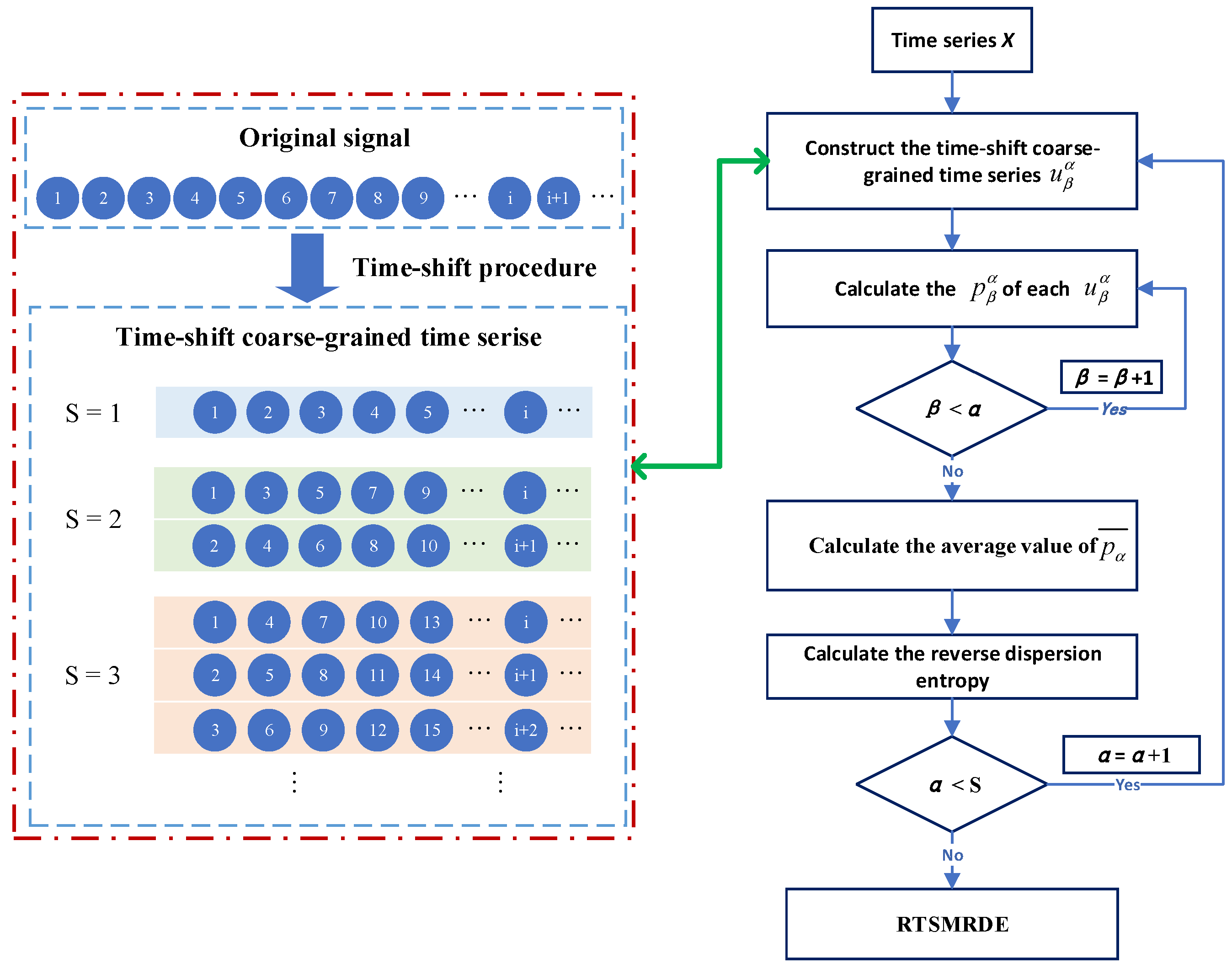
2. Refined Time-Shift Multiscale Reverse Dispersion Entropy

2.1. Reverse Dispersion Entropy

Based on the theory of PE, RDE is a new time-series complexity analysis method that combines the positive aspects of DE and Reverse Permutation Entropy. The following is a description of the RDE steps [20]:
Step 1. Assuming we have a univariate signal of length X = x 1 , x 2 , , x N , X is mapped into Y = y 1 , y 2 , , y N by the standard normal cumulative distribution function (NCDF).
y i = 1 σ 2 π x i e t γ 2 2 σ 2 d t
where y i 0 , 1 ; σ and γ denote the standard deviation and mean of X , respectively.
Step 2. Mapping Y to c classes. We map Y to Z c = z 1 c , z 2 c , , z N c using r o u n d c y i + 0.5 , where c is the number of classes, and z i is a positive integer from 1 to c.
Step 3. Z is reconstructed to embedding vectors T using time delay d and embedding dimension m, respectively. The matrix comprising embedding vectors can be expressed as follows:
z 1 c , z 1 + d c , , z 1 + ( m 1 ) d c           z j c , z j + d c , , z j + ( m 1 ) d c           z t c , z t + d c , , z t + ( m 1 ) d c
where N ( m 1 ) d is the number of embedding vectors t.
Step 4. Each value z j in each vector group corresponds to the subscript of pattern π v o v 1 v m 1 , as shown below:
z j c = v 0 , z j + d c = v 1 , z j + 2 d c = v 2 , , z j + ( m 1 ) d c = v m 1
where c m is the number of potential dispersion patterns, because each z j c has m members, and each one can be an integer between 1 and c.
Step 5. The following is an expression for the ith dispersion pattern’s relative frequency:
p ( π i ) = N u m b e r π i N ( m 1 ) d ( 1 i c m )
where p ( π i ) represents the probability of the ith dispersion patterns.
Step 6. The RDE calculation illustrated below:
R D E ( x , m , c , d ) = i = 1 c m ( p ( π i ) 1 c m ) 2
When p ( π i ) = 1 / c m , the value of R D E ( x , m , c , d ) is 0 (minimum value). When p ( π i ) = 1 , π i is the only existing dispersion pattern, the value of R D E ( x , m , c , d ) is 1 1 / c m (maximum value). Thus, the normalized RDE can be expressed as follows:
N R D E = R D E ( x , m , c , d ) 1 1 / c m

2.2. Multiscale Reverse Dispersion Entropy

MRED is an improved algorithm combining RDE with multiscale entropy. Non-overlapping multiscale means are calculated at different scales to form a new sequence, and then the RDE values are calculated. The MRDE algorithm can be described below.
For time series X = x 1 , x 2 , , x N , the initial time series X is divided into non-overlapping segments of length s. Then, the mean of each segment is calculated, and they are arranged in order together. This process is called coarse graining, as shown below:
y j s = 1 s i = j 1 s + 1 j s x i , 1 j L / s
where s is scale factor. When s = 1 , y 1 is the initial time series. When s > 1 , the original sequence is divided into s coarse graining sequences of length L / s .
For each set of coarse graining data, RDE is calculated as:
M R D E X , m , c , d , s = R D E y s , m , c , d
MRDE analysis is used to calculate the RDE of the coarse-grained sequence under multiple scales. The method overcomes the limitation of RDE in measuring the complexity of signals only at a single scale. MRDE uses a coarse-grained multiscale process, but it has a high requirement for the length of the time series. When the scale factor increases, the length of the coarse-grained sequence becomes shorter, which may result in larger errors. In other words, during the coarse-graining process, the original signal is blurred into multiple signals, which simplifies the calculation but also poses a risk of ignoring important fault information.

2.3. Refined Time-Shift Multiscale Reverse Dispersion Entropy

In this subsection, RTSMRDE is proposed aiming at the above problems of MRDE, and the detailed steps of RTSMRDE can be described as follows:
For time series X = x 1 , x 2 , , x N , β and α are positive integers, where β = 1 , 2 , , α ; then, α new time series can be constructed by:
u β α = x β , x β + α , x β + 2 α , , x β + N β / α α
where α is the time-shift interval; N β / α represents positive integers less than or equal to N β / α .
For a given scale factor α, u β α is composed of N / α signal points. Thus, the p β α π v 0 v 1 v m 1 of each u β α can be acquired using RDE. Then, we define the probability average of time-shift multiscale coarse-grained sequences when scale equal to α.
p α ¯ π v 0 v 1 v m 1 = 1 α β = 1 α p β α π v 0 v 1 v m 1
The final RTSMRDE value at scale α as follow:
R T S M R D E X , m , c , d , α = i = 1 c m ( p β α ¯ ( π v 0 v 1 v m 1 ) 1 c m ) 2
The RTSMRDE algorithm processes the original sequence using time-shift methods to form a sequence group consisting of multiple sub-sequences, each of which is still a part of the original sequence. This maximally preserves the information in the original signal, and the mean probability of the dispersion patterns also resolves the error caused by the increasing scale factor. The flowchart of RTSMRDE is shown as Figure 1.

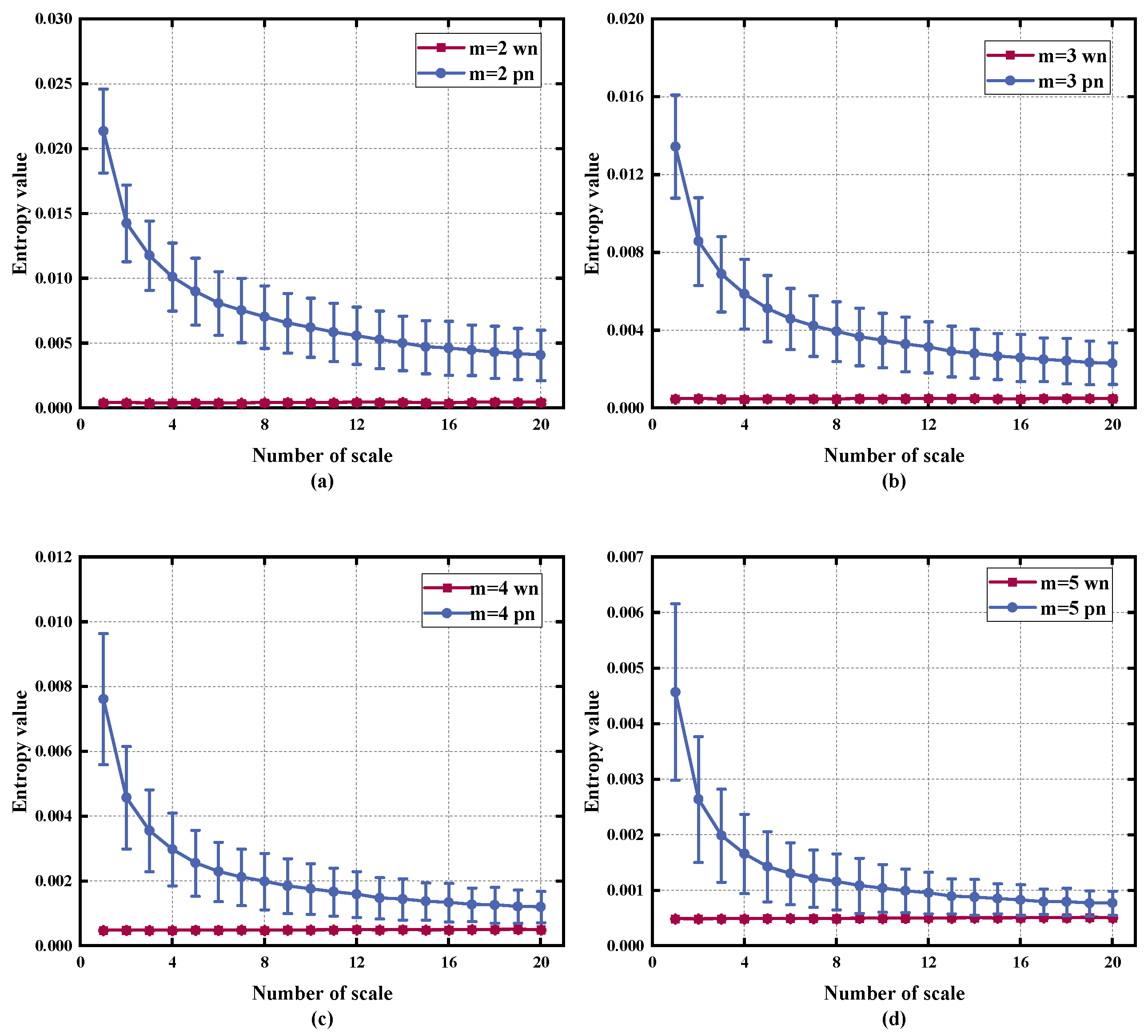
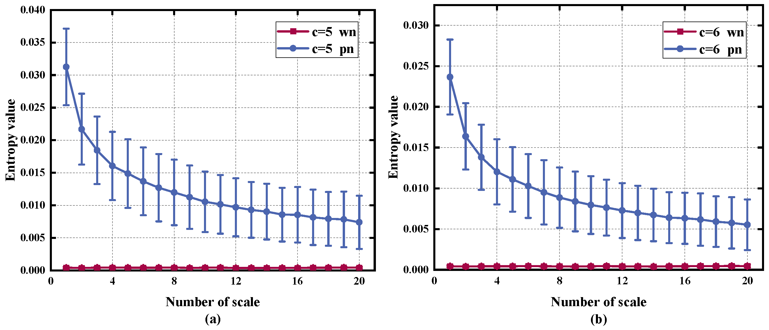
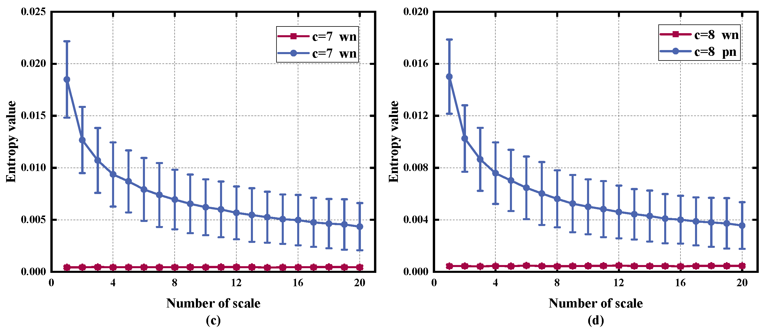
2.4. Parameters Selection

There are four parameters for the RTSMRDE that must be manually configured, namely the scale s, the time delay d, the embedding dimension m, and the class c. In total, 30 sets of pink noise (pn) and white noise (wn) were used as test signals. In machine fault detection, white noise refers to a random noise signal with uniform power spectral density whose energy in the frequency domain is basically equal in each frequency band and has no obvious frequency distribution characteristics; pink noise is a type of noise signal with a 1/f power spectral density distribution characteristic, and the energy in its low-frequency part is more than that in the high-frequency part.
First, we considered how the algorithm would be affected by the time delay d and scaling factor s. According to [20], there may be confusion when the time delay d exceeds 1, even though the impact of time delay on the algorithm is minimal. Therefore, we decided to set the time delay to 1. In addition, choosing an incorrect scale factor s could pose a challenge in accurately extracting the signal’s fault feature information. If the scale factor is too large, it can negatively impact the algorithm’s performance and generate inaccurate entropy values. In order to obtain reliable results, we chose to comprehensively consider a scale factor of 20.
Second, we considered the impact of the embedding dimension m on the RTSMRDE algorithm. Regarding the selection of the embedding dimension m, if it is set too small, it may be difficult to detect the dynamic behaviour of the signal. As shown in Figure 2, the entropy values of both the signal and the noise decrease with increasing m, but the general pattern remains the same. However, as shown in Table 1, increasing m will require more processing time. Moreover, the entropy values between different noises tend to converge at larger scales. Therefore, we decided to set m equal to 2.
Finally, we considered the impact of varying values of c on the algorithm, with m set to 2. If c is set too small, it will be challenging to distinguish between classes with varying amplitudes. On the other hand, a large value of c can increase the system’s susceptibility to noise and result in a higher computational load. Figure 3 shows that, despite a decrease in the entropy values of the two noises with higher c values, the overall trend remained largely unchanged. However, setting too many categories can significantly increase the computation time, as shown in Table 2. Therefore, to strike a balance between reliable statistical measurements and computational efficiency, we decided to set the number of categories c equal to 6.
In conclusion, the appropriate values for the RTSMRDE parameters were m = 2, c = 6, d = 1, and s = 20.

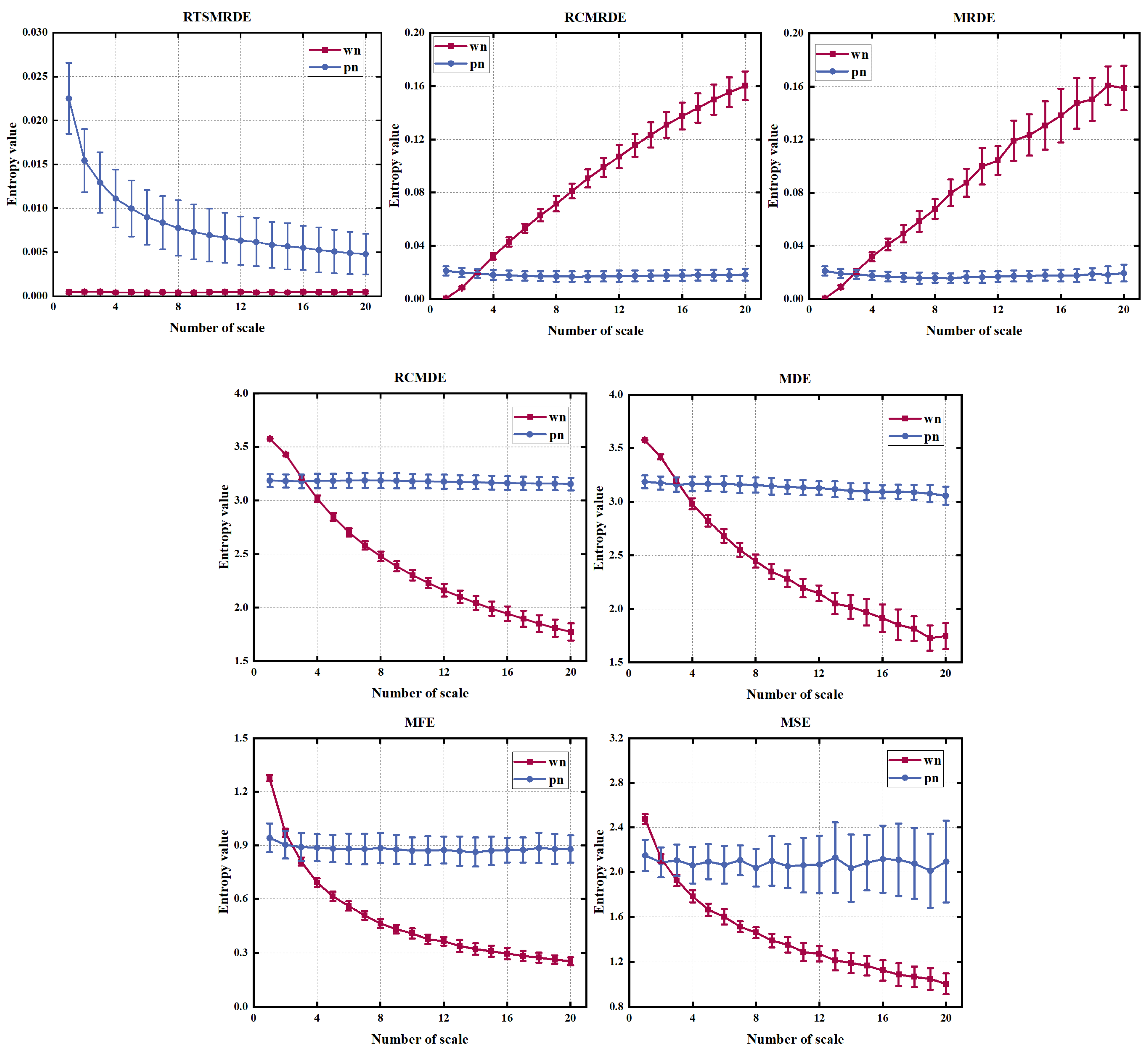
2.5. Comparison of RTSMRDE and Other Entropy Methods Using White Noise and Pink Noise

We compared our proposed method to other existing entropy algorithms, with specific parameters listed in Table 3. For the convenience of comparison, we set the scale factor of the seven algorithms to 20. White noise and pink noise, each configured with 30 samples, were used for the comparison. The running times and results of the seven entropy algorithms are presented in Table 4 and Figure 4, respectively.
As shown in Figure 4, the entropy curves calculated by MSE, MFE, MDE, and MRDE exhibited significant fluctuations with the increasing scale. Among them, MSE and MRDE also showed an increasing error at larger scale factors. In contrast, the entropy values derived by the entropy algorithm following refinement operation and composite coarse-grained structure were more stable. In addition, RTSMRDE combined with the time-shifted structure could correctly distinguish the two noises at full scale, and no crossover occurred. Furthermore, the reverse dispersion entropy was defined as the distance of the signal from the white noise, and only the white noise value of RTSMRDE was closest to 0 among RTSMRDE, RCMRDE, and MRDE, which was consistent with the reality. Finally, Table 4 shows that MDE and MRDE had the shortest calculation time. RTSMRDE had the next shortest time. The calculation time of the other methods was three to four times that of RTSMRDE. In conclusion, the RTSMRDE is of superior quality than the comparative algorithms mentioned above.

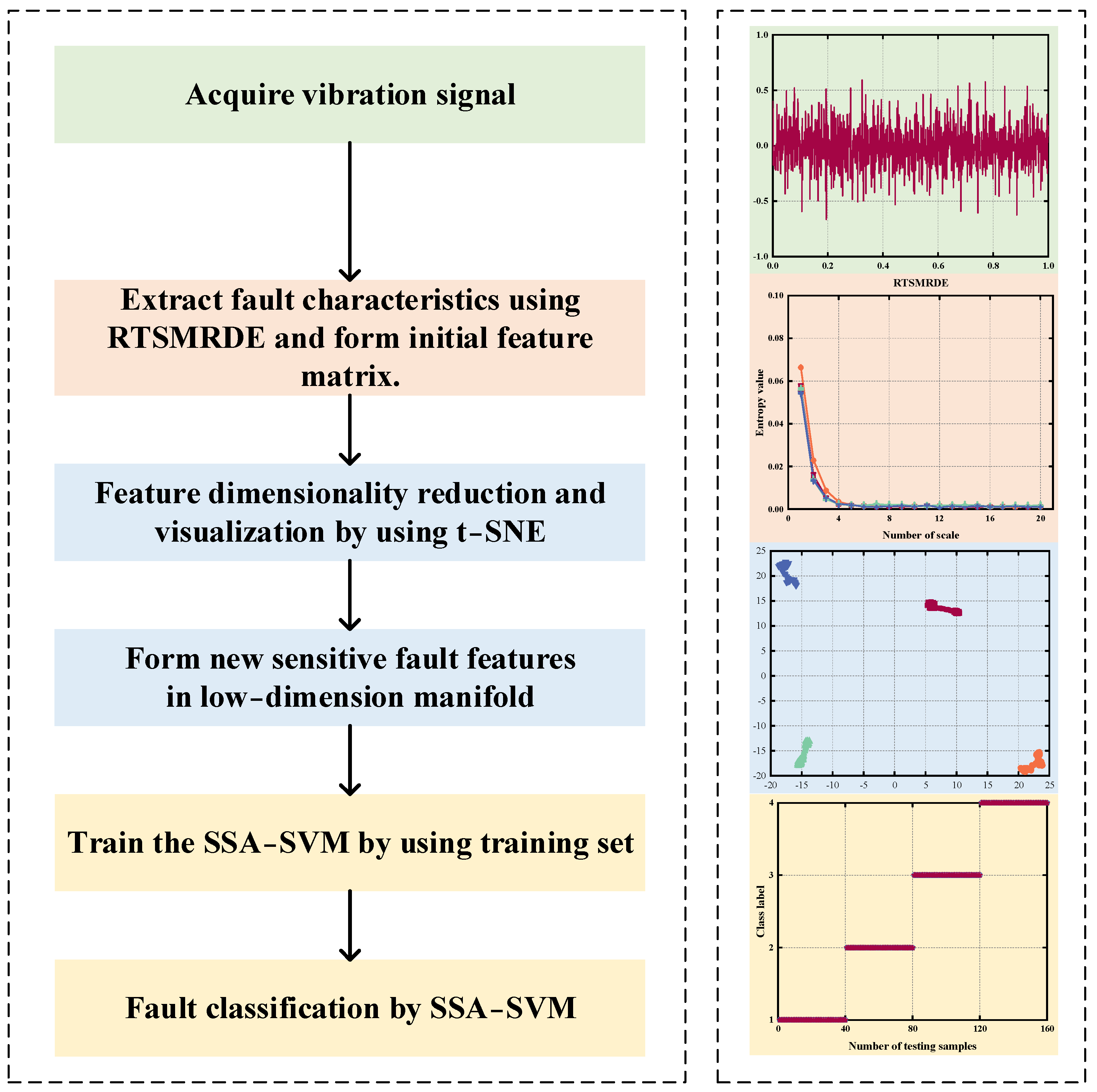
3. The Proposed Intelligent Gearbox Fault Diagnosis Method

3.1. Data Reduction Method

The t-SNE is a nonlinear dimensionality reduction algorithm commonly used for the dimensionality reduction and visualization of high-dimensional data. The algorithm maps high-dimensional data into low-dimensional space, so that the relative distance between data points can be preserved, and the effect of dimensionality reduction and visualization is achieved. Specifically, the t-SNE algorithm defines similarity matrices in high-dimensional and low-dimensional spaces, respectively, and optimizes the mapping relationship by minimizing the Kullback–Leibler divergence between the two similarity matrices. Through the gradient descent algorithm, each data point in the high-dimensional space is mapped to the corresponding data point in the low-dimensional space. Compared with the traditional linear dimensionality reduction algorithm, the t-SNE algorithm can preserve the local structure information between data more completely, so it performs better in visualizing high-dimensional data. More detailed algorithm steps can be found in the relevant literature [27].

3.2. Support Vector Machine

SVM is an efficient classification model. The basic idea of SVM is to find an optimal hyperplane in the feature space, which separates the samples of different classes and maximizes the margin between different samples. In SVM, the sample points closest to the hyperplane determine the location of the hyperplane. Those sample points are called support vectors. The ultimate goal of SVM optimization is to find the hyperplane with the largest margin and minimize the classification error. For non-linearly separable data sets, slack variables are usually introduced, or kernel functions are used to map the data into high-dimensional space. The specific algorithm of SVM can be referred to in [33].

3.3. Sparrow Search Algorithm

The SSA simulates the foraging and anti-predator behaviour of sparrows and establishes a mathematical model flexibly using producer and scavenger strategies. The specific theoretical method can be referred to in [35], and its mathematical model can be briefly described as follows.
Represent the position of sparrows using the following matrix:
M = M 1 , 1 M 1 , 2 M 1 , y M 2 , 1 M 2 , 2 M 2 , y M x , 1 M x , 2 M x , y
where x is the number of sparrows, and y is the number of optimization parameters.
The fitness value of all sparrows can be expressed by matrix below:
F M = f M 1 , 1 M 1 , 2 M 1 , y f M 2 , 1 M 2 , 2 M 2 , y f M x , 1 M x , 2 M x , y
where F M represents the fitness value.
During the search process, producers with higher fitness have higher priority in obtaining food. The location update of the producer is described as:
M i , j t + 1 = M i , j t exp x α i t e r max M i , j t + Q L R 2 < S T R 2 S T
where t represents the iteration number; X i , j t represents the ith sparrow in the jth dimension after t iterations; i t e r max is a constant representing the maximum number of iterations; R 2 and ST are the alarm value and safety threshold, respectively; α is a random number between 0 and 1; Q is a random number following normal distribution. L is a matrix of size 1 × y with all elements equal to 1.
The scroungers need to monitor the producers’ predation. When producers have food, they will compete for it. If the scroungers fail, they will continue to monitor. The update of the scrounger’s position is shown as follows:
M i , j t + 1 = Q exp M w o r s t t M i , j t i 2 i > n 2 M P t + 1 + M i , j t M P t + 1 A + L i n 2
where A represents a matrix whose elements are either 1 or −1, and A + = A T A A T 1 ; M p is the best position located by the producer; M w o r s t represents the current worst position. When i > n / 2 , it means that ith scrounger has a risk of insufficient energy.
The initial position of sparrows in the population is randomly generated, the formula is shown below:
M i , j t + 1 = M b e s t t + β M i , j t M b e s t t f i > f g M i , j t + K M i , j t M w o r s t t f i f w + ε f i = f g
where M b e s t represents the current global optimal location; β is the step control parameter; the value of K is between −1 and 1; f i is the fitness value; f w and f g represent the current worst and best adaptation, respectively; ε is the minimum constant. When f i > f g , this indicates that the sparrow is at the edge of the group; when f i = f g , this indicates that the sparrows in the middle of the population realize the danger and need to be closer to other sparrows.

3.4. The Proposed Fault Diagnosis Scheme

Based on RTSMRDE, t-SNE and SSA-SVM, the flowchart of proposed method is shown in Figure 5. The steps are summarized as follows:
First, the rotating machinery fault experimental platform collected the gearbox vibration signals under various failure conditions.
Second, the proposed RTSMRDE was used to compute the entropy values and create a high-dimensional feature set in order to completely extract the feature information of the gearbox fault signals.
Third, the dimensionality of the initial RTSMRDE feature set was reduced using the t-SNE to generate a sensitive low-dimensional feature set.
Finally, an optimized SVM model was constructed using SSA. The test set was fed into the optimized SVM for fault classification.

4. Experimental Verification

Through two gearbox fault experiments, the performance of the proposed fault diagnostic technique was evaluated. In addition, the proposed fault diagnosis model was compared with the existing diagnosis algorithm to verify its superior performance. All experiments were performed on the MATLAB R2022a environment running on an AMD Ryzen 7 5800 H 3.2 GHz, 16.0 GB RAM, and Windows 11 computer.

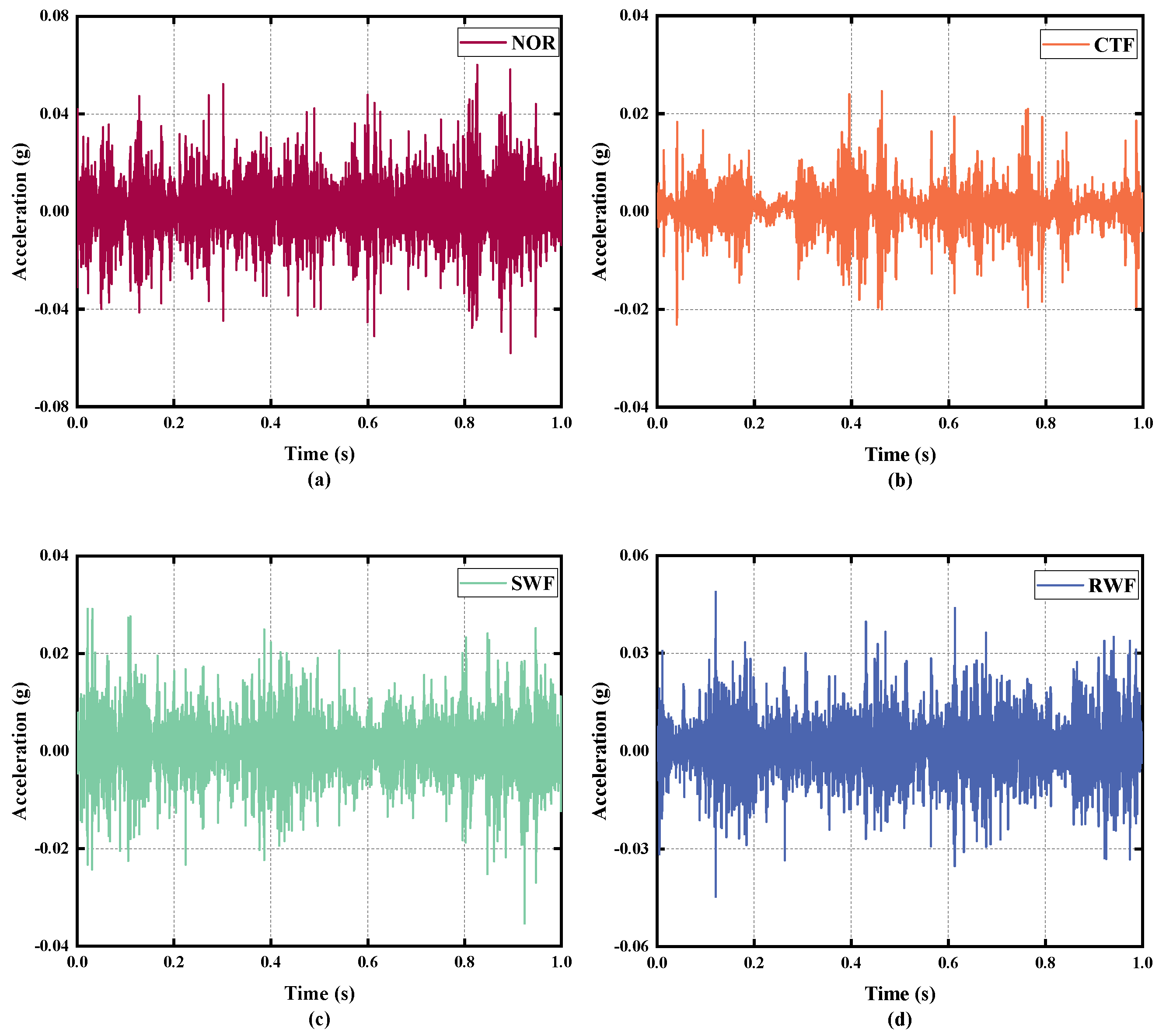
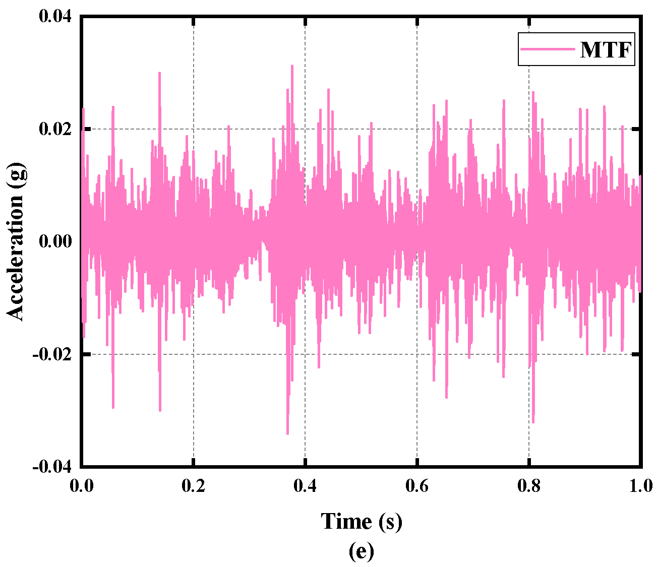
4.1. Case 1: Data from Southeast University Gearbox Dataset

4.1.1. Description and Division of Data

The experimental data (D1) of the gearbox in Case One were provided by Southeast University [42]. Dataset D1 selected the vibration signal collected by the Y-axis sensor on the planetary gearbox in the original dataset, which was operated under the condition that the load of the speed system was set to 20 Hz–0 V. As shown in Table 5, the D1 dataset had five operating states, namely Normal, Chipped tooth, Surface wear, Root wear, and Missing tooth. Each operating state consisted of 50 sub-samples with a data length of 2048. Therefore, there was a total of 250 samples in dataset D1. These samples were divided into 10 training samples and 40 testing samples for fault diagnosis. The time-domain signals of the five operating states are shown in Figure 6, where it can be clearly seen that there were obvious impact components in the time-domain waveform under faulty conditions.

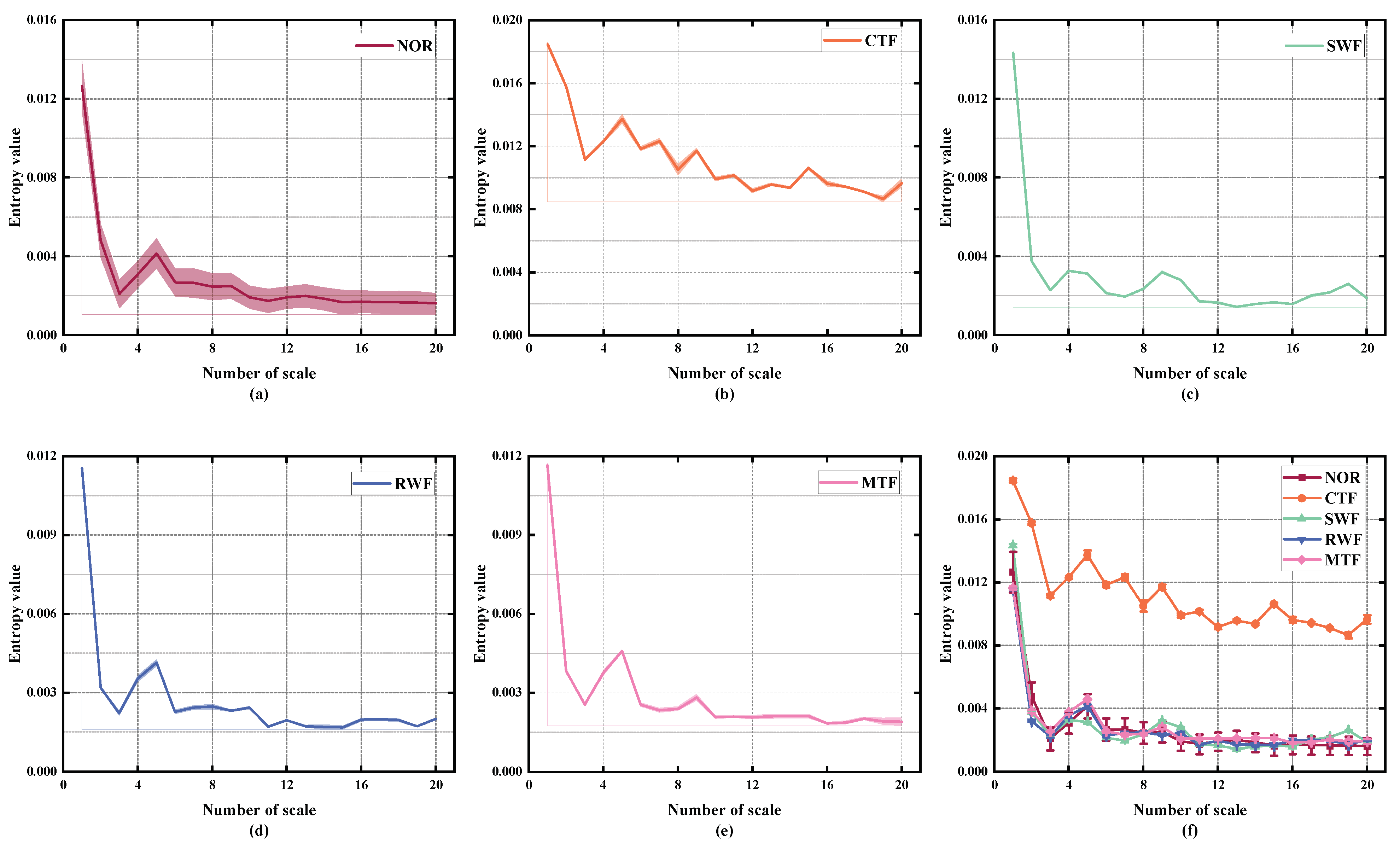
4.1.2. Feature Extraction for D1

Using the RTSMRDE as a feature extraction tool, fault features were extracted from the experimental dataset D1 consisting of 250 samples. In the end, we obtained a 250 × 20 fault feature matrix, where 250 is the number of samples and 20 is the dimension of feature extraction. Figure 7 shows the error bar plot of entropy calculation for dataset D1. It can be seen from the figure that the trends of the five fault states in the multiscale calculation were the same and stable; except for a small error in the normal state, the errors in the other states were almost invisible. This indicates that the RTSMRDE algorithm can effectively overcome the defects of entropy calculation in multiscale and control the entropy bias phenomenon.

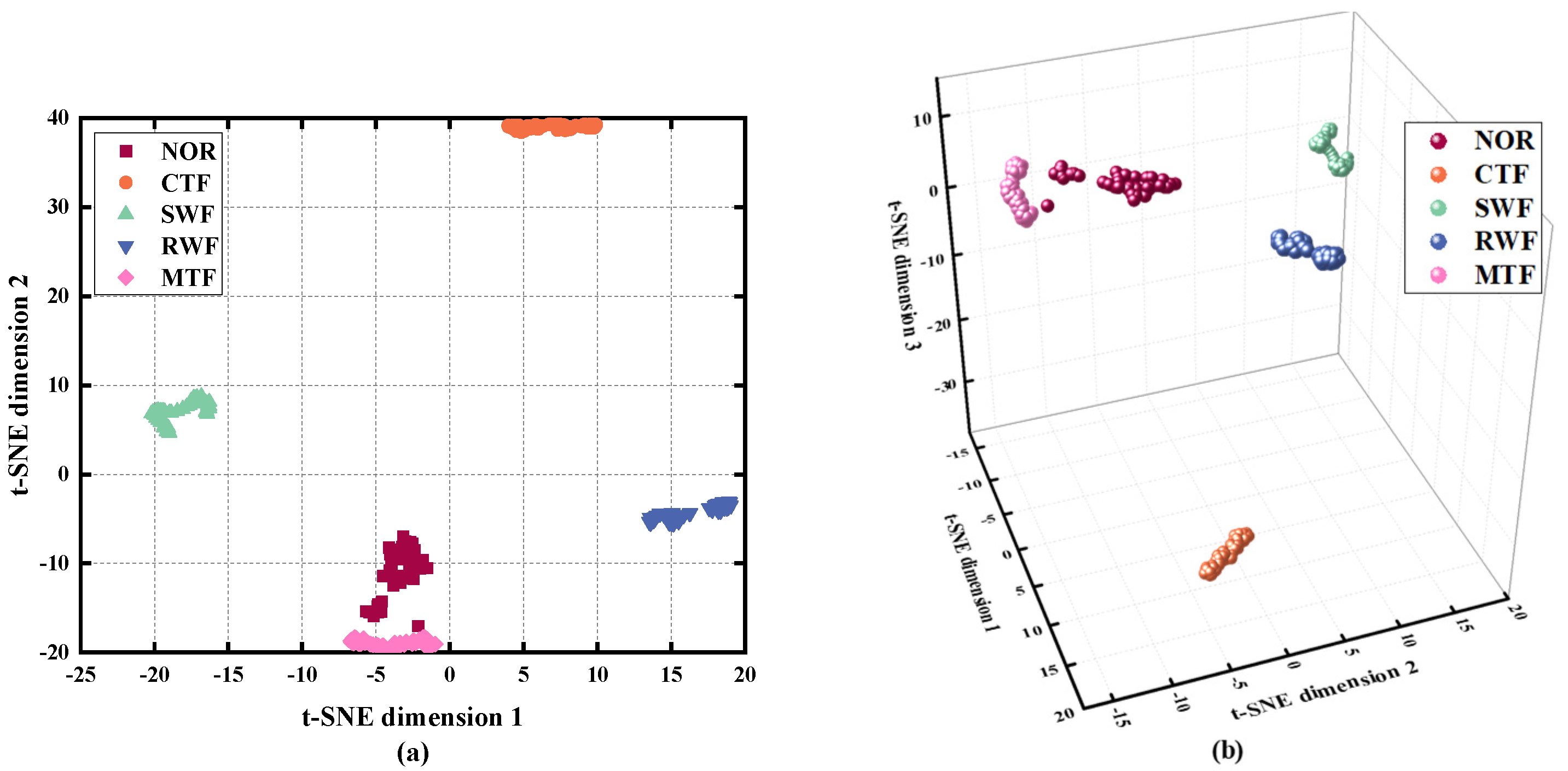
4.1.3. Data Reduction and Visualization

Relying solely on the entropy curve to determine the fault status of the gearbox is a challenging task. Therefore, the t-SNE dimension reduction algorithm was employed to process the high-dimensional feature set. The reduced fault feature set only consisted of the most sensitive fault features, which not only saved time in computation but also facilitated visualization. As shown in the Figure 8, the visual results of the sample features obtained after two-dimensional and three-dimensional dimension reduction show that each group of samples was well-clustered, with no sample mixing or blurred boundaries observed among the five operating status samples of the gearbox. These results indicate that the t-SNE algorithm is capable of effectively extracting crucial information from high-dimensional features and accurately identifying the status of the gearbox.

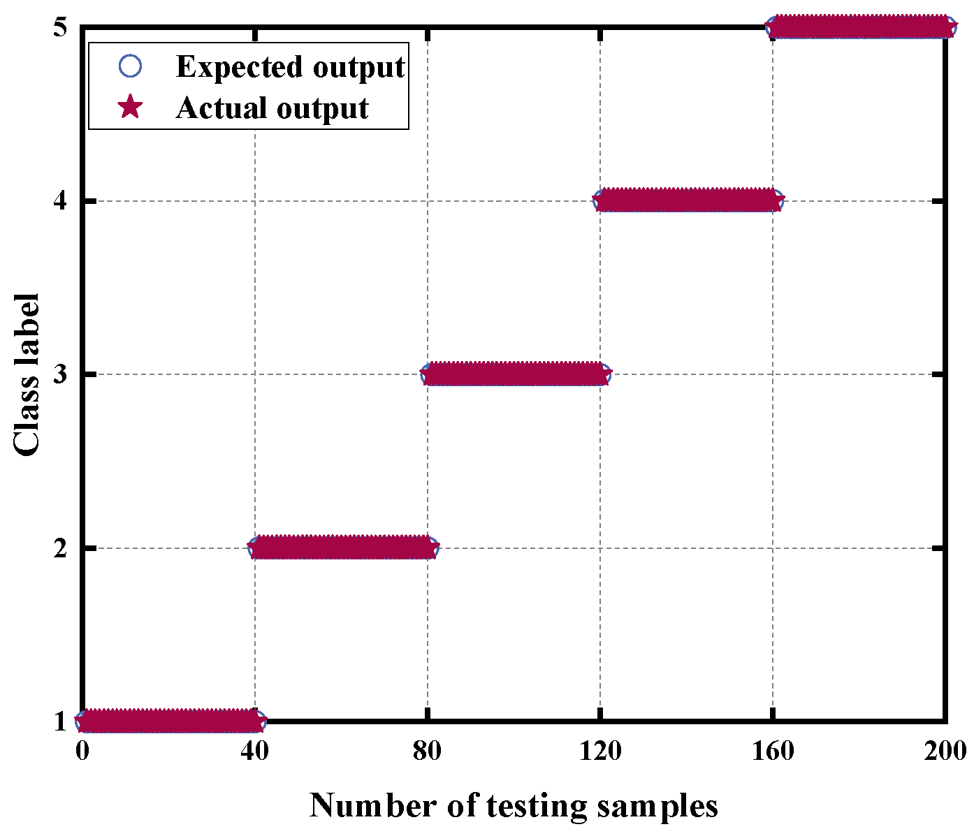
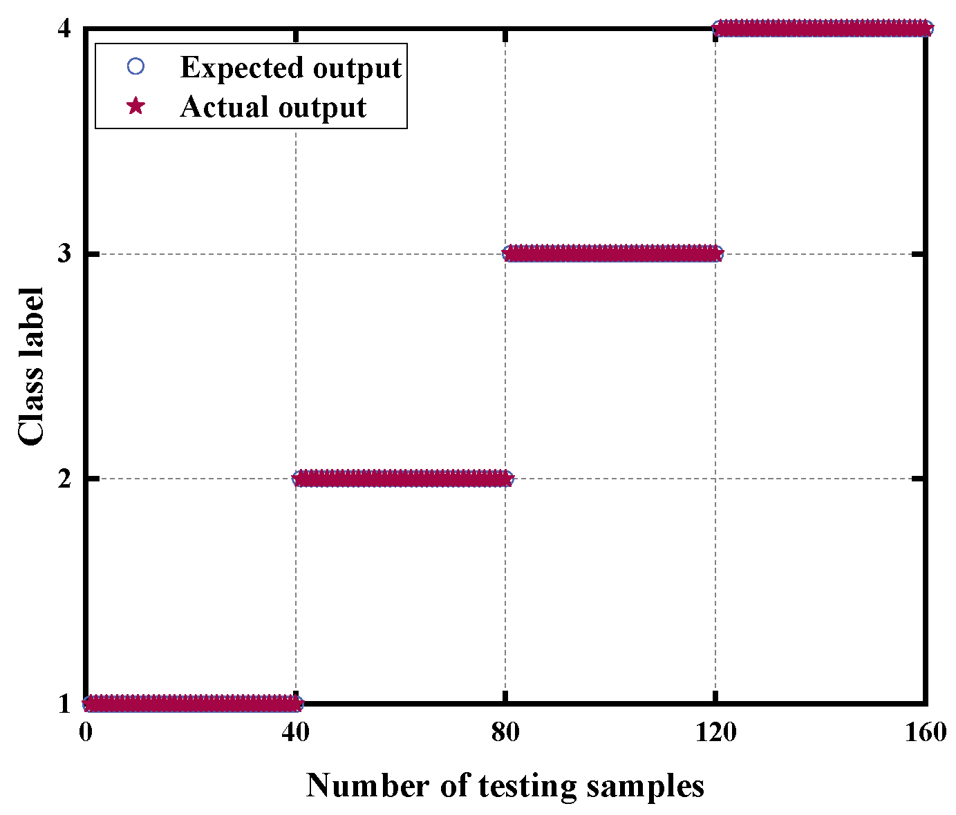
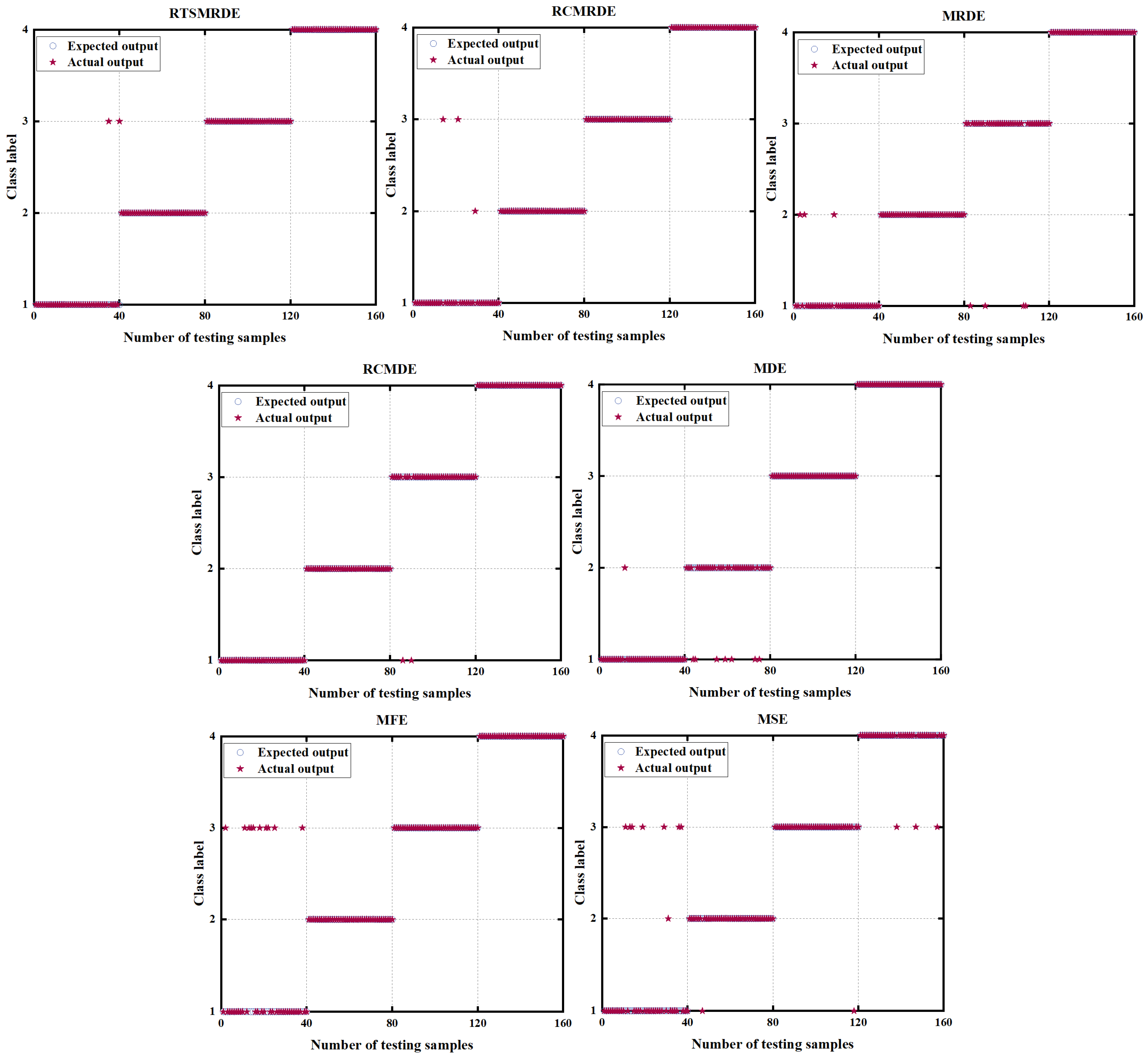
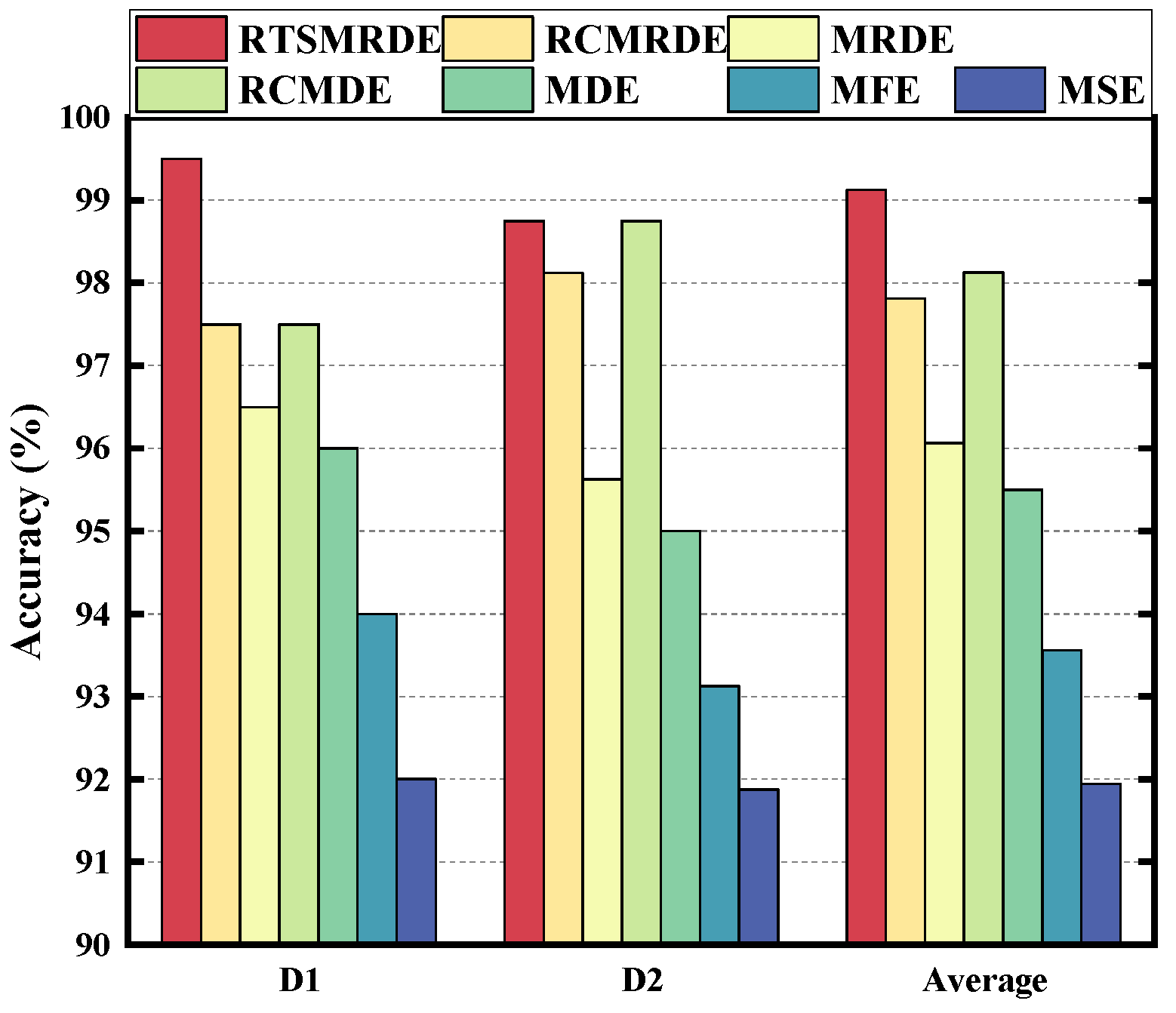
4.1.4. Analysis of Diagnosis Results

Finally, the intelligent diagnosis of the gearbox faults was achieved by inputting the low-dimensional sensitive feature set into SSA-SVM. To train the model, 10 sets of samples for each state were randomly selected as the training set, and the remaining 40 sets were used as the test set. There was a total of 50 training samples and 200 test samples. The SSA was used to optimize the SVM parameters. Then, the optimized support vector machine model was established, and the test set was input into the model for classification. As shown in the Figure 9, the proposed method could effectively identify various faults with a recognition accuracy of up to 100%.

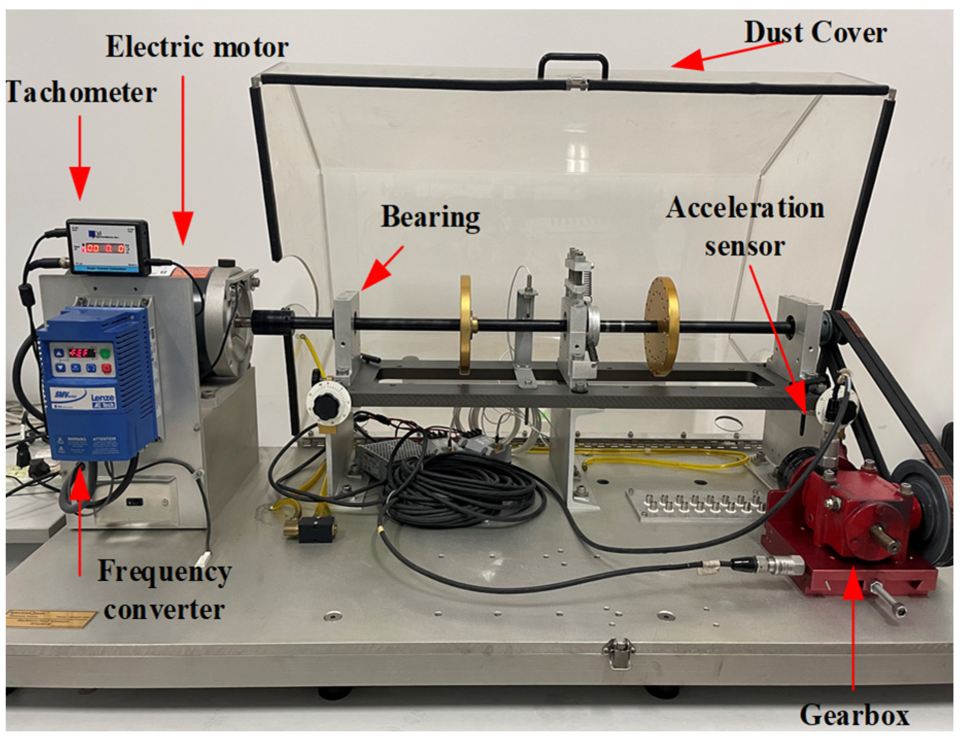
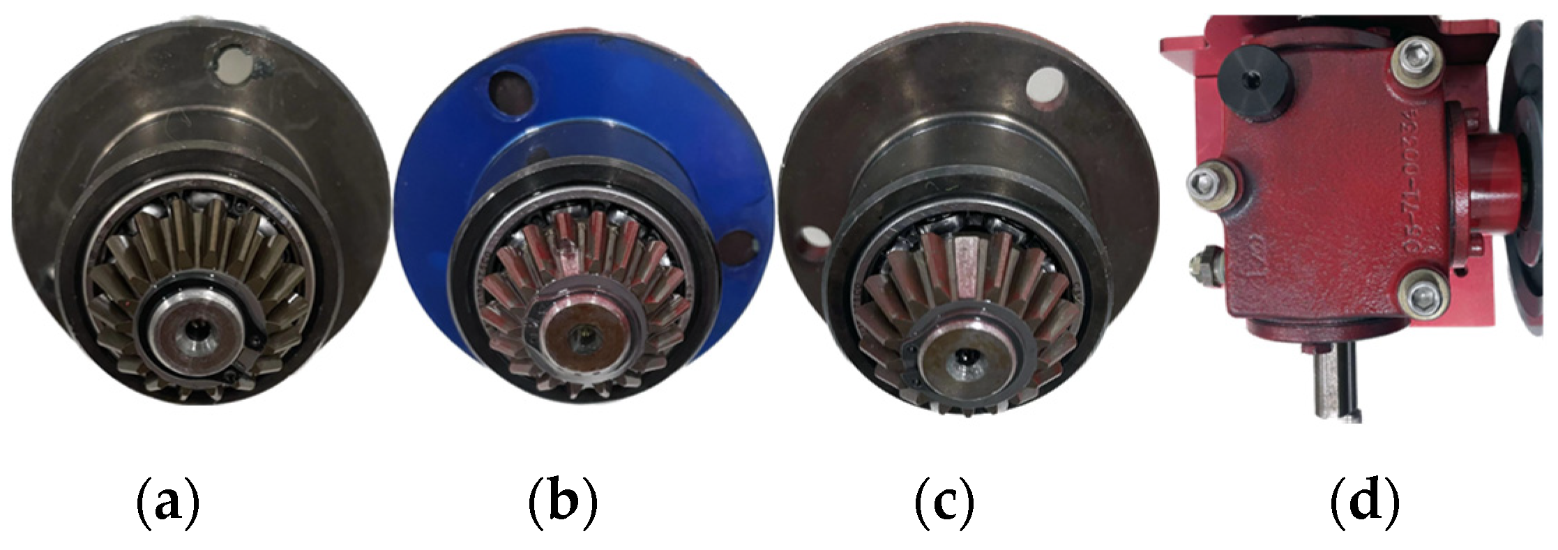
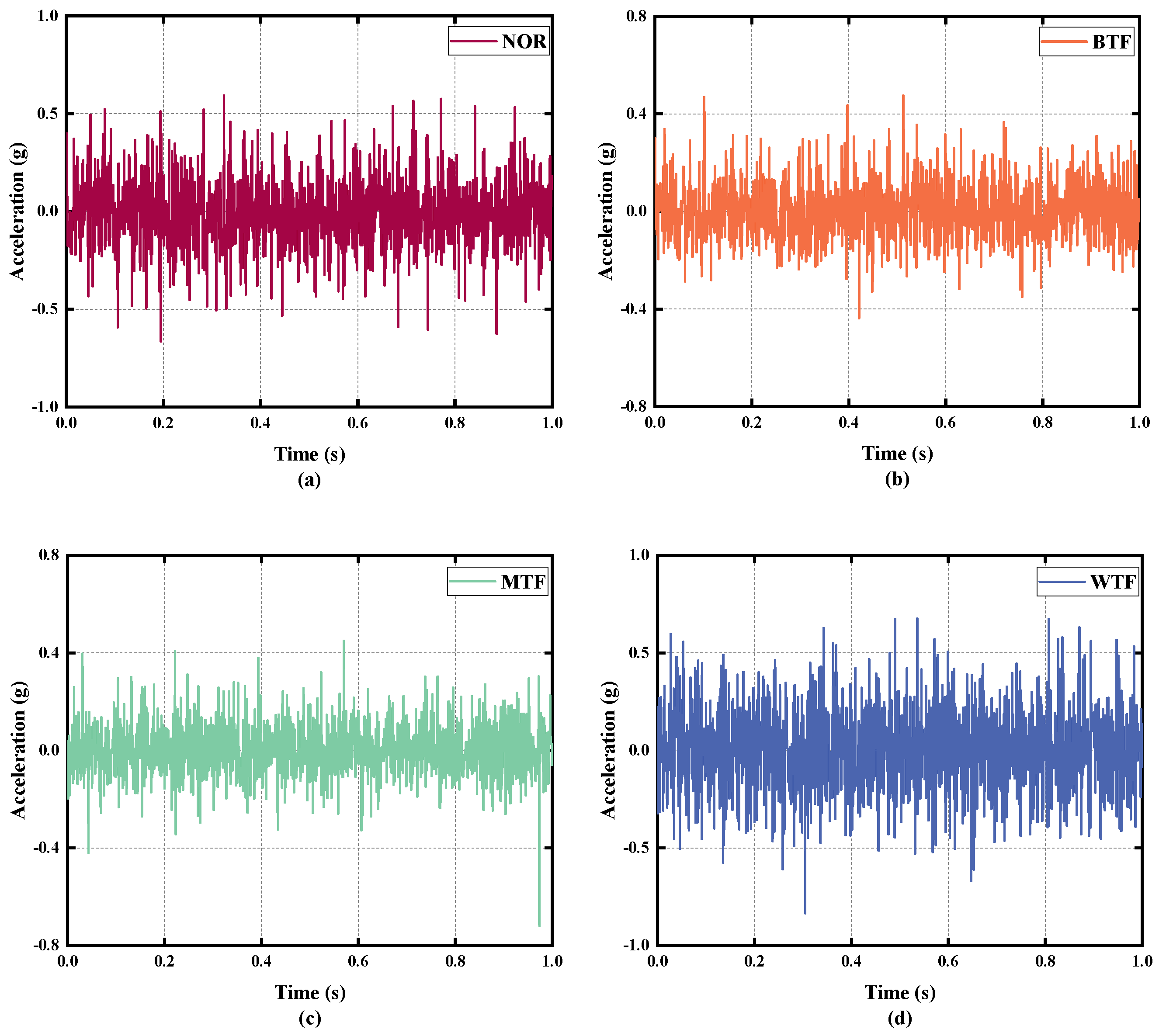
4.2. Case 2: Data from MFS

4.2.1. Description and Division of Data

The gearbox data set (D2) was provided by a mechanical failure simulation experiment system (MFS). The MFS manufactured by SQI company can simulate various common mechanical equipment, and the modular component design of the experimental bench is powerful and reliable, so it can be used to simulate common bearing and gear failures of the wind turbine drive train. As shown in Figure 10, the main part of the experimental system consisted of the integrated mechanical fault simulation experimental bench and the data acquisition equipment. As shown in Figure 11, the gearbox fault diagnosis study kit used for the experiment consisted of a missing tooth fault gear, a broken tooth fault gear, and a tooth wear gearbox.
The experiments were conducted at a motor speed of 1750 rpm to test the normal state and three fault states, respectively. The original samples were divided into 50 sub-samples, and each sample was 2048 in length. The D1 is shown in Table 6. The vibration signals of four faults are shown in Figure 12.

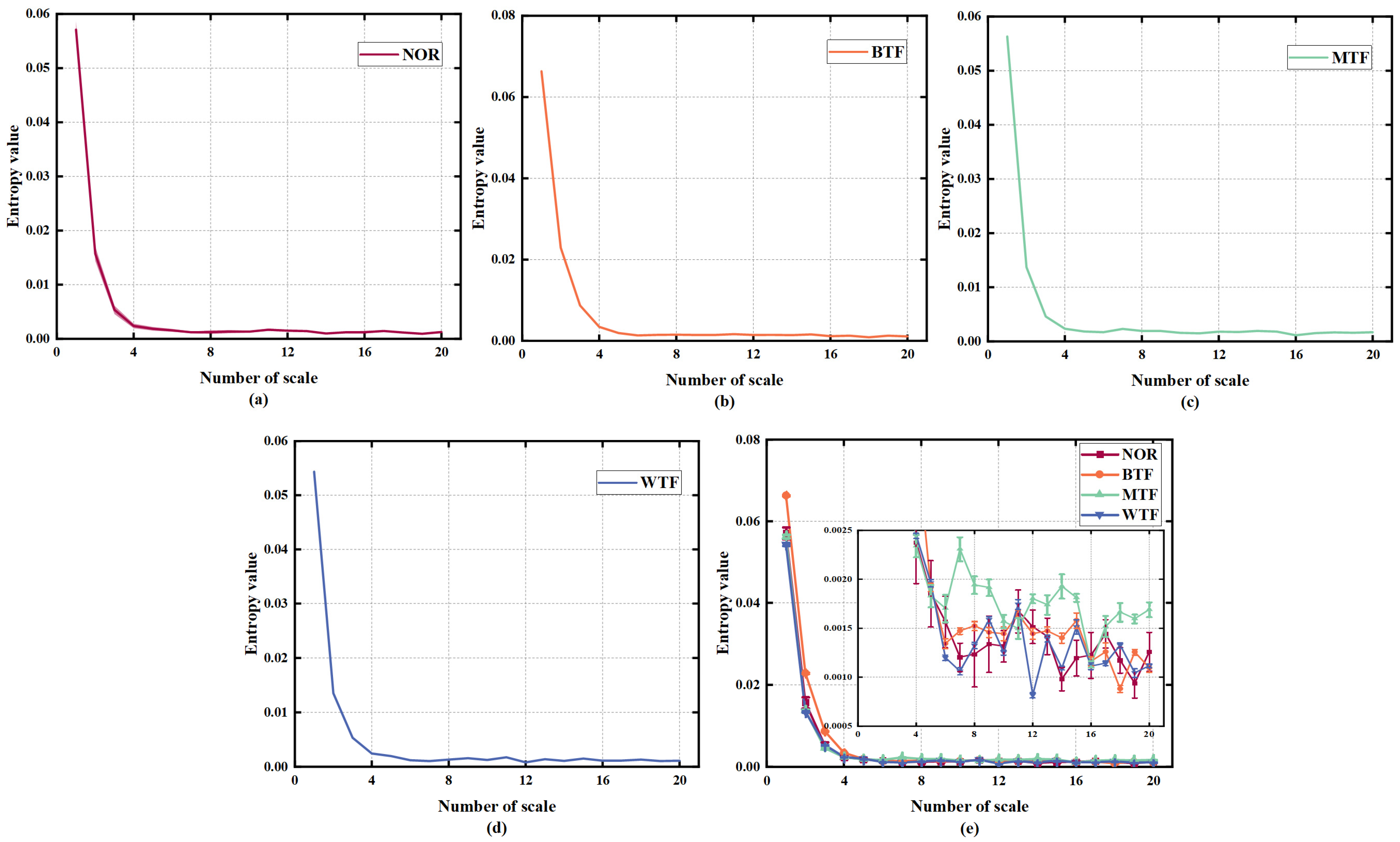
4.2.2. Feature Extraction for D2

The MFS experimental platform collected vibration signals from four faults and selected 50 sample signals for each fault. The entropy value was calculated for these 200 samples, and the RTSMRDE algorithm was used to extract feature from the fault signals. The resulting fault feature matrix had a size of 200 × 20, where 200 represents the number of samples and 20 represents the number of dimensions. As shown in the Figure 13, the RTSMRDE values indicate a stable trend, and the error value was extremely small, making it nearly invisible in the error bar graph. Zooming in on the region of scale range from 4 to 20 in Figure 13e, it can be seen that the entropy values calculated for the four fault states were not equal but existed in an alternating manner. Although using RTSMRDE can make the results of entropy calculation more stable and reduce entropy bias, directly using a high-dimensional feature matrix for classification cannot produce the best results.

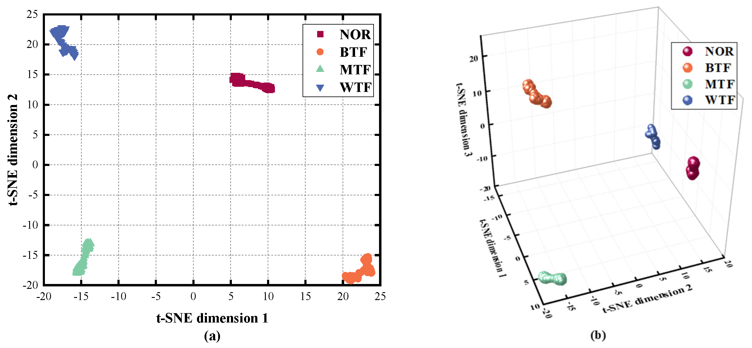
4.2.3. Data Reduction and Visualization

Using the t-SNE algorithm to reduce the size of the initial feature matrix of 200 × 20, the visualization results of the dimensionality reduction are shown in Figure 14, and the four fault states are clearly distinguished. Each fault state signal existed independently in different regions without confusion. The 2D and 3D visualization results both showed ideal results. This indicates that the t-SNE algorithm can effectively extract key information from high-dimensional features, making it easier to distinguish the state of the gearbox.

4.2.4. Analysis of Diagnosis Results

The fault classification was achieved using SSA-SVM. As shown in the Figure 15, the method proposed in this paper could effectively identify various faults with a recognition accuracy of up to 100%.

4.3. Contrast Analysis

To fully verify the advantages of the proposed fault diagnosis model, we used two sets of control experiments to compare the advantages of RTSMRDE and data dimension reduction in the fault diagnosis model.

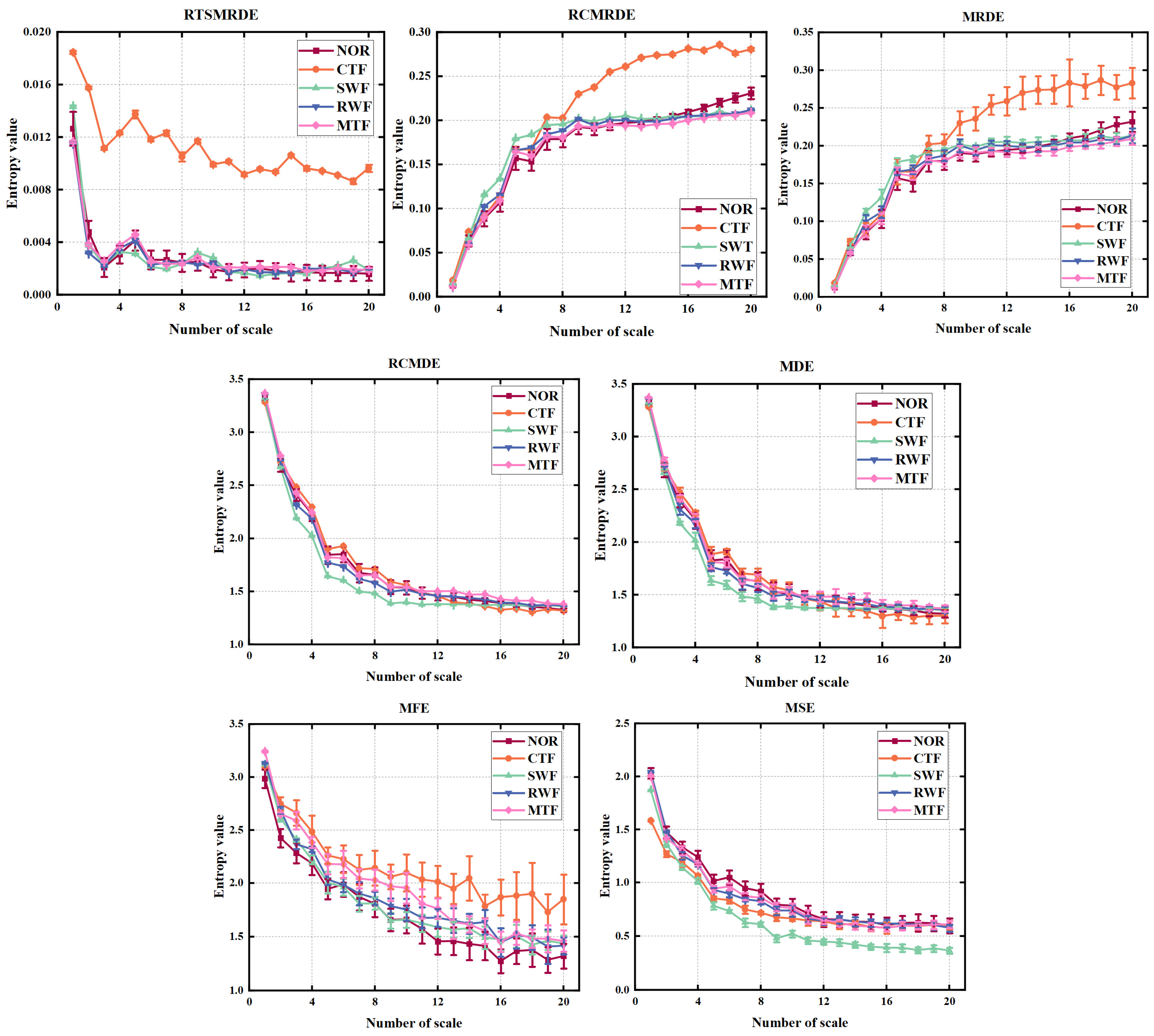
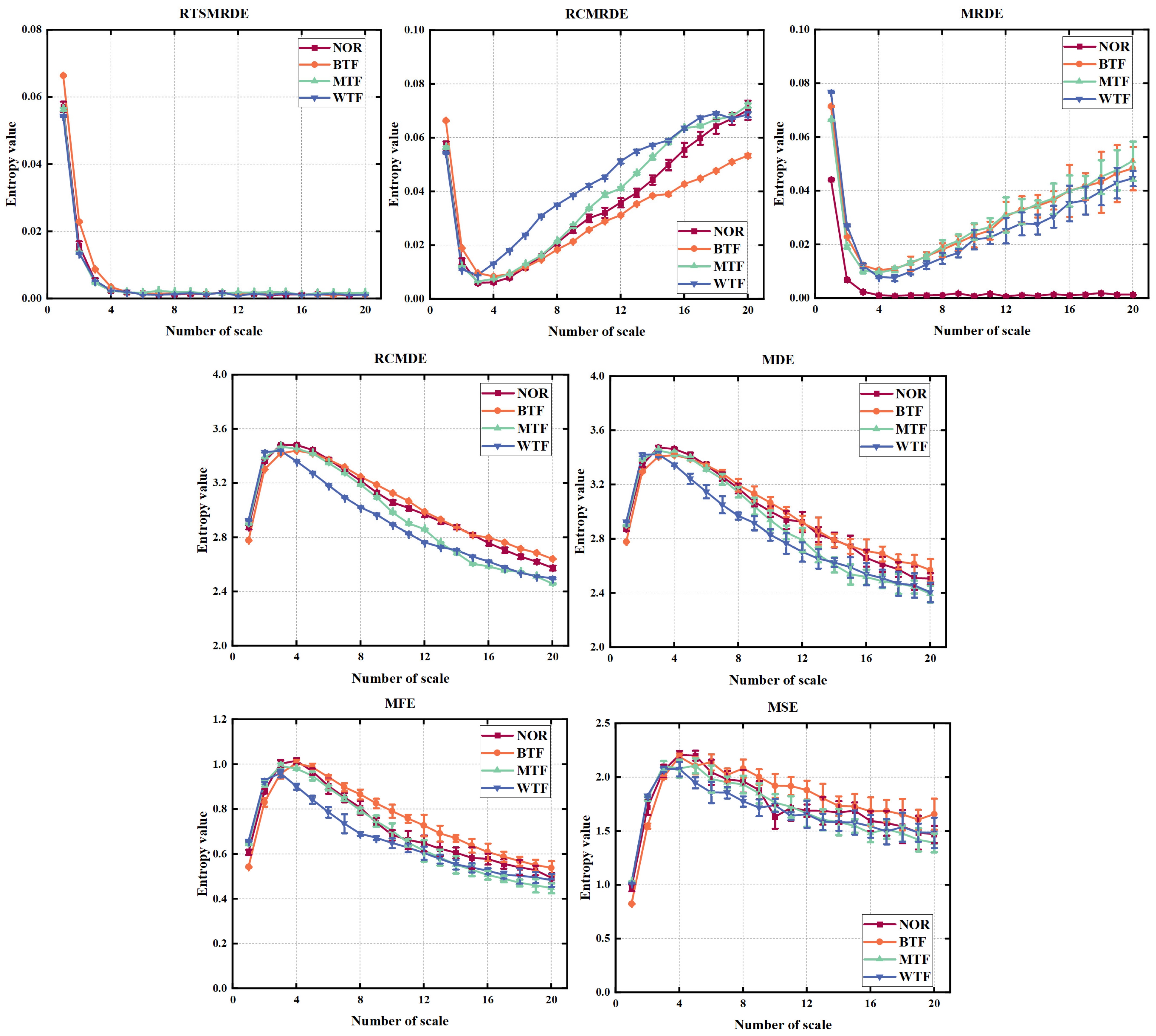
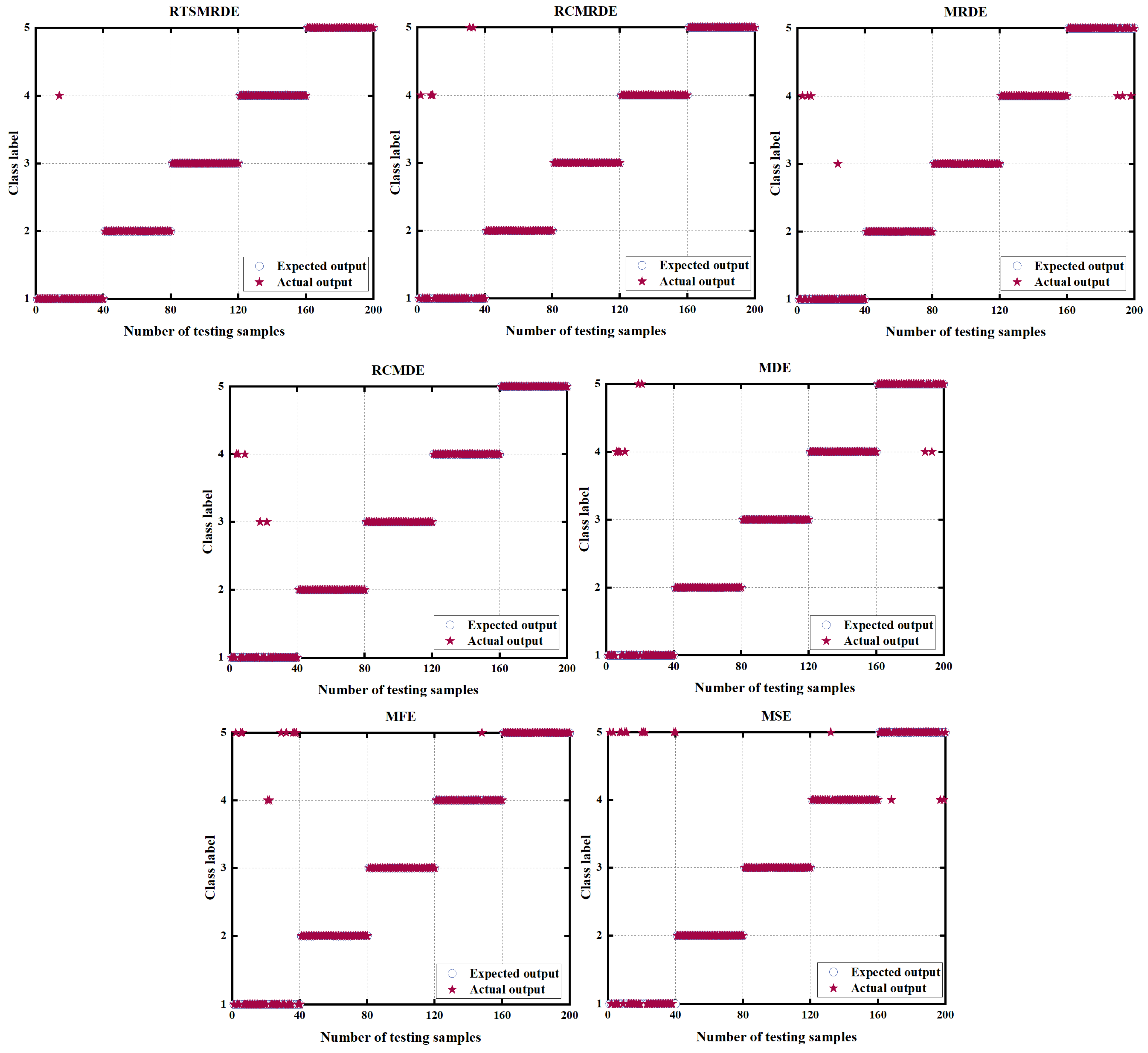
4.3.1. Comparison of RTSMRDE with Other Different Entropy Algorithms

To verify the advantages of the RTSMRDE, it was compared with six other entropy algorithms mentioned in Table 3 using the D1 and D2 dataset. The entropy calculation results of each algorithm are shown in Figure 16 and Figure 17, respectively. The entropy values calculated by the MSE, MFE, MDE, and MRDE algorithms showed increasing errors with increasing scale, and the entropy curves showed significant fluctuations. However, the refined composite entropy algorithm showed smaller errors and smoother curves, indicating that the algorithm is more stable and effective. The entropy curve calculated by the samples processed by the refined time-shift algorithm showed the smallest error and the most stable curve among all the results, indicating the best performance.
The feature sets extracted by each algorithm were sent to the SSA-SVM for classification, and the results are shown in Figure 18 and Figure 19, respectively. As shown in Figure 18, the numbers of the misclassified samples for RTSMRDE, RCMRDE, MRDE, RCMDE, MDE, MFE, and MSE on D1 were 1, 5, 7, 5, 8, 11, and 15, respectively. The average correct rate of the RTSMRDE algorithm was 99.5%, which was the highest among the seven algorithms, with accuracy rates of 2%, 3%, 2%, 3.5%, 5.5%, and 7.5% higher than the other six algorithms, respectively. As shown in the Figure 19, the numbers of the misclassified samples for RTSMRDE, RCMRDE, MRDE, RCMDE, MDE, MFE, and MSE on D2 were 2, 3, 7, 2, 8, 10, and 13, respectively. The RTSMRDE algorithm exhibited an average correct rate of 98.75%, surpassing the other six algorithms by 0.625%, 3.125%, 0%, 3.75%, 5.625%, and 6.875% in terms of accuracy rates.
Figure 20 shows the accuracy of different algorithms on two datasets. In addition, the running time of each algorithm is shown in Table 7. It is clear that the MDE and MRDE algorithms had the shortest computation time of approximately 2 s. The RTSMRDE algorithm took approximately 4 s, which was the second shortest. The computation time of other algorithms exceeded 10 s, which was three to four times longer than that of RTSMRDE. In summary, the proposed method performed better for fault classification of the gearbox dataset.

4.3.2. Comparison between Using and Not Using Data Reduction Methods

By comparing Figure 9 and Figure 15, the first subfigures of Figure 17, and the first subfigure of Figure 18, it can be observed that the classification result obtained without using data dimension reduction algorithm had one misclassified sample in D1 and two misclassified samples in D2. However, after applying the data dimension reduction algorithm, all samples could be correctly classified. This indicates that the sensitive feature set extracted through data reduction can effectively improve the classification accuracy.

5. Conclusions

The vibration signal of a gearbox has non-continuous and non-linear characteristics. When a gearbox local fault occurs, periodic fault signals with impact characteristics will appear. Therefore, we proposed a feature extraction method based on RTSMRDE, t-SNE, and SSA-SVM to construct a new intelligent diagnosis method for gearbox faults. The effectiveness and superiority of this method compared to existing methods were verified through simulation signals and fault simulation experiments. The proposed method had a positive impact on the fault diagnosis of rotating components, such as gearboxes in wind turbines. The following conclusions have been drawn:
  • The RTSMRDE is based on MRDE, combined with the ideas of time shifting coarse-graining operations. It overcomes the shortcomings of traditional multiscale reverse dispersion entropy and can effectively and comprehensively extract the fault characteristics of gearboxes.
  • The t-SNE can effectively remove redundant features in high-dimensional fault feature sets, thus obtaining a sensitive and easily classifiable low-dimensional feature set.
  • Constructing a novel diagnosis model for gearbox faults based on RTSMRDE, t-SNE, and SSA-SVM.
  • The proposed method was validated with noise signals and experimental datasets and demonstrated a more prominent overall performance in terms of feature extraction capability and computational speed.

Author Contributions

Conceptualization, X.W. and H.J.; methodology, X.W. and H.J.; validation, X.W. and H.J.; investigation, X.W. and H.J.; resources, X.W.; data curation, X.W. and H.J.; writing—original draft preparation, H.J.; writing—review and editing, X.W.; visualization, H.J.; supervision, X.W.; project administration, X.W.; funding acquisition, X.W. All authors have read and agreed to the published version of the manuscript.

Funding

The project of software and hardware development of online vibration condition monitoring and intelligent fault diagnosis for rotating machinery (3612403222440) supported by scientific research Foundation of Nanjing Institute of Technology.

Data Availability Statement

The data presented in this study are available on request from the corresponding author.

Conflicts of Interest

The authors declare no conflict of interests.

Abbreviations

The following abbreviations are used in this manuscript:
MSEMultiscale Sample Entropy
MFEMultiscale Fuzzy Entropy
MPEMultiscale Permutation Entropy
DEDispersion Entropy
MDEMultiscale Dispersion Entropy
RCMDERefined Composite Multiscale Dispersion Entropy
RDEReverse Dispersion Entropy
MRDEMultiscale Reverse Dispersion Entropy
RCMRDERefined Composite Multiscale Reverse Dispersion Entropy
RTSMRDERefined Time-Shifted Multiscale Reverse Dispersion Entropy
t-SNEt-distributed Stochastic Neighbour Embedding
SSA-SVMSparrow Search Algorithm-Support Vector Machine
PNpink noise
WNwhite noise

References

  1. Cheng, Y.; Zhu, H.; Wu, J.; Shao, X. Machine Health Monitoring Using Adaptive Kernel Spectral Clustering and Deep Long Short-Term Memory Recurrent Neural Networks. IEEE Trans. Ind. Inform. 2018, 15, 987–997. [Google Scholar] [CrossRef]
  2. Liu, R.; Yang, B.; Zio, E.; Chen, X. Artificial intelligence for fault diagnosis of rotating machinery: A review. Mech. Syst. Signal Process. 2018, 108, 33–47. [Google Scholar] [CrossRef]
  3. Xu, X.; Qiao, Z.; Lei, Y. Repetitive transient extraction for machinery fault diagnosis using multiscale fractional order entropy infogram. Mech. Syst. Signal Process. 2018, 103, 312–326. [Google Scholar] [CrossRef]
  4. Zheng, J.D.; Pan, H.Y. Use of generalized refined composite multiscale fractional dispersion entropy to diagnose the faults of rolling bearing. Nonlinear Dyn. 2020, 101, 1417–1440. [Google Scholar] [CrossRef]
  5. Zhang, W.; Li, X.; Ma, H.; Luo, Z.; Li, X. Federated learning for machinery fault diagnosis with dynamic validation and self-supervision. Knowl.-Based Syst. 2021, 213, 106679. [Google Scholar] [CrossRef]
  6. Tian, Y.; Wang, Z.; Lu, C. Self-adaptive bearing fault diagnosis based on permutation entropy and manifold-based dynamic time warping. Mech. Syst. Signal Process. 2019, 114, 658–673. [Google Scholar] [CrossRef]
  7. Vakharia, V.; Gupta, V.; Kankar, P. A multiscale permutation entropy based approach to select wavelet for fault diagnosis of ball bearings. J. Vib. Control 2014, 21, 3123–3131. [Google Scholar] [CrossRef]
  8. Jia, Y.; Xu, M.; Wang, R. Symbolic Important Point Perceptually and Hidden Markov Model Based Hydraulic Pump Fault Diagnosis Method. Sensors 2018, 18, 4460. [Google Scholar] [CrossRef] [Green Version]
  9. Li, Y.; Wang, X.; Liu, Z.; Liang, X.; Si, S. The Entropy Algorithm and Its Variants in the Fault Diagnosis of Rotating Machinery: A Review. IEEE Access 2018, 6, 66723–66741. [Google Scholar] [CrossRef]
  10. Pincus, S.M. Approximate entropy as a measure of system complexity. Proc. Natl. Acad. Sci. USA 1991, 88, 2297–2301. [Google Scholar] [CrossRef] [Green Version]
  11. Khoshnami, A.; Sadeghkhani, I. Sample entropy-based fault detection for photovoltaic arrays. IET Renew. Power Gener. 2018, 12, 1966–1976. [Google Scholar] [CrossRef]
  12. Zheng, J.; Pan, H.; Cheng, J. Rolling bearing fault detection and diagnosis based on composite multiscale fuzzy entropy and ensemble support vector machines. Mech. Syst. Signal Process. 2017, 85, 746–759. [Google Scholar] [CrossRef]
  13. Dong, Z.; Zheng, J.; Huang, S.; Pan, H.; Liu, Q. Time-Shift Multi-scale Weighted Permutation Entropy and GWO-SVM Based Fault Diagnosis Approach for Rolling Bearing. Entropy 2019, 21, 621. [Google Scholar] [CrossRef] [Green Version]
  14. Costa, M.; Goldberger, A.L.; Peng, C.-K. Multiscale Entropy Analysis of Complex Physiologic Time Series. Phys. Rev. Lett. 2002, 89, 068102. [Google Scholar] [CrossRef] [Green Version]
  15. Wang, Z.; Yao, L.; Cai, Y. Rolling bearing fault diagnosis using generalized refined composite multiscale sample entropy and optimized support vector machine. Measurement 2020, 156, 107574. [Google Scholar] [CrossRef]
  16. Dangdang, Z.; Han, B.; Liu, G.; Li, Y.; Yu, H. Cross-Domain Intelligent Fault Diagnosis Method of Rotating Machinery Using Multi-Scale Transfer Fuzzy Entropy. IEEE Access 2021, 9, 95481–95492. [Google Scholar] [CrossRef]
  17. Chen, Y.; Chen, Y.; Dai, Q. Gear compound fault detection method based on improved multiscale permutation entropy and local mean decomposition. J. Vibroeng. 2021, 23, 1171–1183. [Google Scholar] [CrossRef]
  18. Rostaghi, M.; Azami, H. Dispersion Entropy: A Measure for Time-Series Analysis. IEEE Signal Process. Lett. 2016, 23, 610–614. [Google Scholar] [CrossRef]
  19. Azami, H.; Escudero, J. Amplitude- and Fluctuation-Based Dispersion Entropy. Entropy 2018, 20, 210. [Google Scholar] [CrossRef] [Green Version]
  20. Li, Y.; Gao, X.; Wang, L. Reverse Dispersion Entropy: A New Complexity Measure for Sensor Signal. Sensors 2019, 19, 5203. [Google Scholar] [CrossRef] [Green Version]
  21. Xing, J.; Xu, J. An Improved Incipient Fault Diagnosis Method of Bearing Damage Based on Hierarchical Multi-Scale Reverse Dispersion Entropy. Entropy 2022, 24, 770. [Google Scholar] [CrossRef] [PubMed]
  22. Zheng, J.; Pan, H.; Liu, Q.; Ding, K. Refined time-shift multiscale normalised dispersion entropy and its application to fault diagnosis of rolling bearing. Phys. A Stat. Mech. Its Appl. 2019, 545, 123641. [Google Scholar] [CrossRef]
  23. Azami, H.; Rostaghi, M.; Abásolo, D.; Escudero, J. Refined Composite Multiscale Dispersion Entropy and its Application to Biomedical Signals. IEEE Trans. Biomed. Eng. 2017, 64, 2872–2879. [Google Scholar] [CrossRef] [Green Version]
  24. Grbovic, M.; Li, W.; Xu, P.; Usadi, A.K.; Song, L.; Vucetic, S. Decentralized fault detection and diagnosis via sparse PCA based decomposition and Maximum Entropy decision fusion. J. Process Control 2012, 22, 738–750. [Google Scholar] [CrossRef]
  25. Li, D.; Hu, G.; Spanos, C.J. A data-driven strategy for detection and diagnosis of building chiller faults using linear discriminant analysis. Energy Build. 2016, 128, 519–529. [Google Scholar] [CrossRef]
  26. Shao, H.; Jiang, H.; Li, X.; Liang, T. Rolling bearing fault detection using continuous deep belief network with locally linear embedding. Comput. Ind. 2018, 96, 27–39. [Google Scholar] [CrossRef]
  27. Tu, D.; Zheng, J.; Jiang, Z.; Pan, H. Multiscale Distribution Entropy and t-Distributed Stochastic Neighbor Embedding-Based Fault Diagnosis of Rolling Bearings. Entropy 2018, 20, 360. [Google Scholar] [CrossRef] [Green Version]
  28. Yin, A.; Lu, J.; Dai, Z.; Li, J.; Ouyang, Q. Isomap and Deep Belief Network-Based Machine Health Combined Assessment Model. Stroj. Vestn.-J. Mech. Eng. 2016, 62, 740–750. [Google Scholar] [CrossRef]
  29. Zheng, J.; Jiang, Z.; Pan, H. Sigmoid-based refined composite multiscale fuzzy entropy and t-SNE based fault diagnosis approach for rolling bearing. Measurement 2018, 129, 332–342. [Google Scholar] [CrossRef]
  30. Li, D.; Gu, M.; Liu, S.; Sun, X.; Gong, L.; Qian, K. Continual learning classification method with the weighted k-nearest neighbor rule for time-varying data space based on the artificial immune system. Knowl.-Based Syst. 2022, 240, 108145. [Google Scholar] [CrossRef]
  31. Wei, Y.; Yang, Y.; Xu, M.; Huang, W. Intelligent fault diagnosis of planetary gearbox based on refined composite hierarchical fuzzy entropy and random forest. ISA Trans. 2020, 109, 340–351. [Google Scholar] [CrossRef]
  32. Saliha, S.; Nabil, E.A. A Novel Hybrid Method Based on Fireworks Algorithm and Artificial Neural Network for Photovoltaic System Fault Diagnosis. Int. J. Renew. Energy Res. 2022, 12, 239–247. [Google Scholar]
  33. Zhang, J.; Zhang, Q.; Qin, X.; Sun, Y. A two-stage fault diagnosis methodology for rotating machinery combining optimized support vector data description and optimized support vector machine. Measurement 2022, 200, 111651. [Google Scholar] [CrossRef]
  34. Chen, H.; Li, S. Multi-Sensor Fusion by CWT-PARAFAC-IPSO-SVM for Intelligent Mechanical Fault Diagnosis. Sensors 2022, 22, 3647. [Google Scholar] [CrossRef] [PubMed]
  35. Xue, J.; Shen, B. A novel swarm intelligence optimization approach: Sparrow search algorithm. Syst. Sci. Control Eng. 2020, 8, 22–34. [Google Scholar] [CrossRef]
  36. Li, W.; Shen, X.; Li, Y. A Comparative Study of Multiscale Sample Entropy and Hierarchical Entropy and Its Application in Feature Extraction for Ship-Radiated Noise. Entropy 2019, 21, 793. [Google Scholar] [CrossRef] [Green Version]
  37. Luo, S.; Yang, W.; Luo, Y. A Novel Fault Detection Scheme Using Improved Inherent Multiscale Fuzzy Entropy With Partly Ensemble Local Characteristic-Scale Decomposition. IEEE Access 2019, 8, 6650–6661. [Google Scholar] [CrossRef]
  38. Zhang, Y.; Tong, S.; Cong, F.; Xu, J. Research of Feature Extraction Method Based on Sparse Reconstruction and Multiscale Dispersion Entropy. Appl. Sci. 2018, 8, 888. [Google Scholar] [CrossRef] [Green Version]
  39. Luo, S.; Yang, W.; Luo, Y. Fault Diagnosis of a Rolling Bearing Based on Adaptive Sparest Narrow-Band Decomposition and RefinedComposite Multiscale Dispersion Entropy. Entropy 2020, 22, 375. [Google Scholar] [CrossRef] [Green Version]
  40. Li, Y.; Jiao, S.; Geng, B.; Zhou, Y. Research on feature extraction of ship-radiated noise based on multi-scale reverse dispersion entropy. Appl. Acoust. 2020, 173, 107737. [Google Scholar] [CrossRef]
  41. Liu, A.; Yang, Z.; Li, H.; Wang, C.; Liu, X. Intelligent Diagnosis of Rolling Element Bearing Based on Refined Composite Multiscale Reverse Dispersion Entropy and Random Forest. Sensors 2022, 22, 2046. [Google Scholar] [CrossRef] [PubMed]
  42. Shao, S.; McAleer, S.; Yan, R.; Baldi, P. Highly Accurate Machine Fault Diagnosis Using Deep Transfer Learning. IEEE Trans. Ind. Inform. 2018, 15, 2446–2455. [Google Scholar] [CrossRef]
Figure 1. The flowchart of the RTSMRDE method.
Machines 11 00646 g001
Figure 2. Different m on RTSMRDE: (a) m = 2, (b) m = 3, (c) m = 4, (d) m = 5.
Machines 11 00646 g002
Figure 3. Different c on RTSMRDE: (a) c = 5, (b) c = 6, (c) c = 7, (d) c = 8.
Machines 11 00646 g003aMachines 11 00646 g003b
Figure 4. Different entropy values on white noise and pink noise.
Machines 11 00646 g004
Figure 5. Flowchart of the fault diagnosis.
Machines 11 00646 g005
Figure 6. The time-domain signals of D1 in the experiment. (a) NOR; (b) CTF; (c) SWF; (d) RWF; (e) MTF.
Machines 11 00646 g006aMachines 11 00646 g006b
Figure 7. RTSMRDE value on D1. (a) NOR; (b) CTF; (c) SWF; (d) RWF; (e) MTF; (f) Five kinds of fault entropy values.
Machines 11 00646 g007
Figure 8. (a) The 2D result obtained using the t-SNE; (b) The 3D result obtained using the t-SNE.
Machines 11 00646 g008
Figure 9. Fault classification of RTSMRDE on D1.
Machines 11 00646 g009
Figure 10. Comprehensive mechanical failure simulation experiment system.
Machines 11 00646 g010
Figure 11. Four gear health states: (a) normal condition; (b) broken tooth fault gear; (c) missing tooth fault gear; (d) the wear tooth gearbox.
Machines 11 00646 g011
Figure 12. The time-domain signals of D2. (a) NOR; (b) BTF; (c) MTF; (d) WTF.
Machines 11 00646 g012
Figure 13. RTSMRDE value on D2. (a) NOR; (b) BTF; (c) MTF; (d) WTF; (e) Four kinds of fault entropy values.
Machines 11 00646 g013
Figure 14. (a) The 2D result obtained using the t-SNE; (b) The 3D result obtained using the t-SNE.
Machines 11 00646 g014
Figure 15. Fault classification of RTSMRDE on D2.
Machines 11 00646 g015
Figure 16. Different entropy values of D1.
Machines 11 00646 g016
Figure 17. Different entropy values of D2.
Machines 11 00646 g017
Figure 18. The fault diagnosis result of D1.
Machines 11 00646 g018
Figure 19. The fault diagnosis result of D2.
Machines 11 00646 g019
Figure 20. Accuracy of different entropy methods.
Machines 11 00646 g020
Table 1. Running time of RTSMRDE for different m values.
Typem = 2m = 3m = 4m = 5
Seconds1.121 s3.403 s14.575 s80.805 s
Table 2. Running time of RTSMRDE for different c.
Typec = 5c = 6c = 7c = 8
Seconds1.025 s1.092 s1.290 s1.549 s
Table 3. Selection of parameters with different entropy.
Entropy MethodsParameters
MSE [36]m = 2, n = 2, d = 1, s = 20, r = 0.15 SD
MFE [37]m = 3, d = 1, s = 20, r = 0.15 SD
MDE [38]m = 3, c = 6, d = 1, s = 20
RCMDE [39]m = 2, c = 9, d = 1, s = 20
MRDE [40]m = 3, c = 5, d = 1, s = 20
RCMRDE [41]m = 2, c = 5, d = 1, s = 20
RTSMRDE (proposed)m = 2, c = 6, d = 1, s = 20
Table 4. Running time for different entropies.
TypeRTSMRDERCMRDEMRDERCMDEMDEMFEMSE
Seconds1.081 s4.576 s0.550 s4.380 s0.549 s4.315 s3.305 s
Table 5. Description of D1.
Fault TypesMotor Speed
(r/min)
Number of
Training Samples
Number of
Testing Samples
Class Label
Normal12001040NOR
Chipped tooth12001040CTF
Surface wear12001040SWF
Root wear12001040RWF
Missing tooth12001040MTF
Table 6. Description of D2.
Fault TypesMotor Speed
(r/min)
Number of
Training Samples
Number of
Testing Samples
Class Label
Normal17501040NOR
Broken tooth17501040BTF
Missing tooth17501040MTF
Wear tooth17501040WTF
Table 7. Running times for different entropies.
DataRTSMRDERCMRDEMRDERCMDEMDEMFEMSE
D14.62 s17.56 s2.40 s17.65 s2.36 s19.26 s14.08 s
D23.76 s14.23 s1.81 s14.36 s1.83 s15.77 s12.22 s
Disclaimer/Publisher’s Note: The statements, opinions and data contained in all publications are solely those of the individual author(s) and contributor(s) and not of MDPI and/or the editor(s). MDPI and/or the editor(s) disclaim responsibility for any injury to people or property resulting from any ideas, methods, instructions or products referred to in the content.

