

Turning Chatter Detection Using a Multi-Input Convolutional Neural Network via Image and Sound Signal
 , ,
, ,
Abstract
:1. Introduction
2. Material and Method
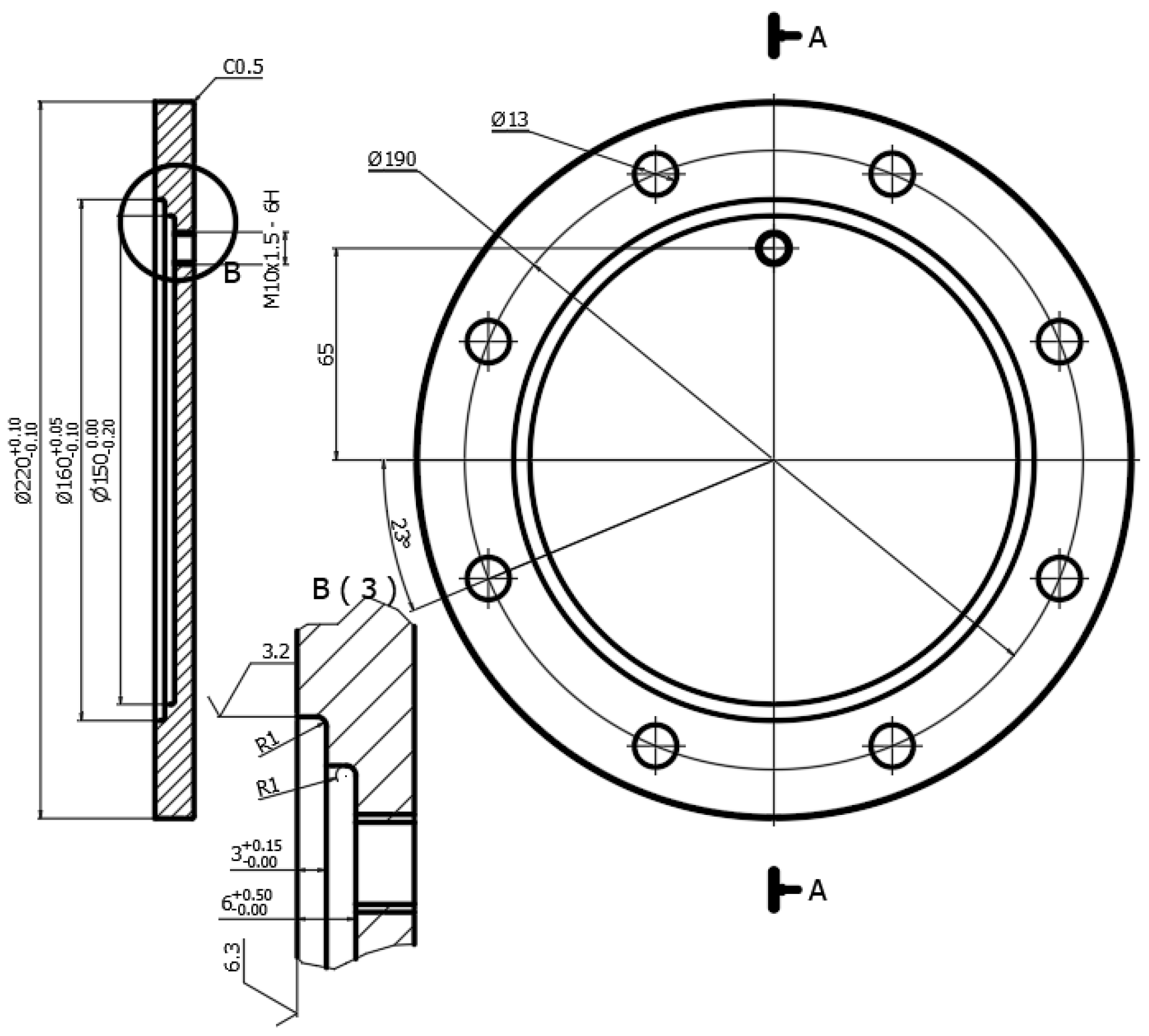
2.1. Material
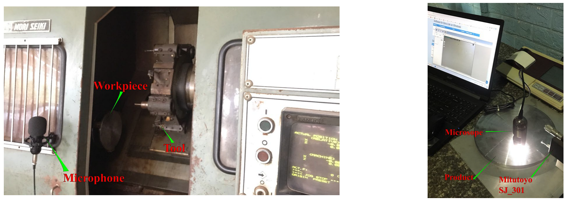
2.2. Signal Acquisition and Processing Devices
2.3. Classification Models
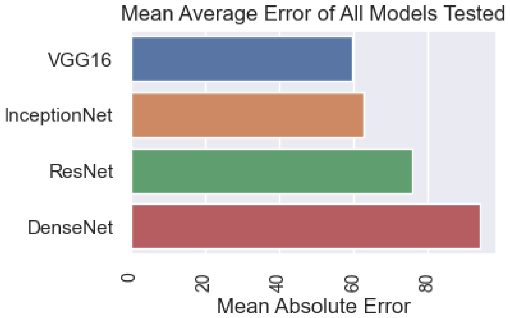
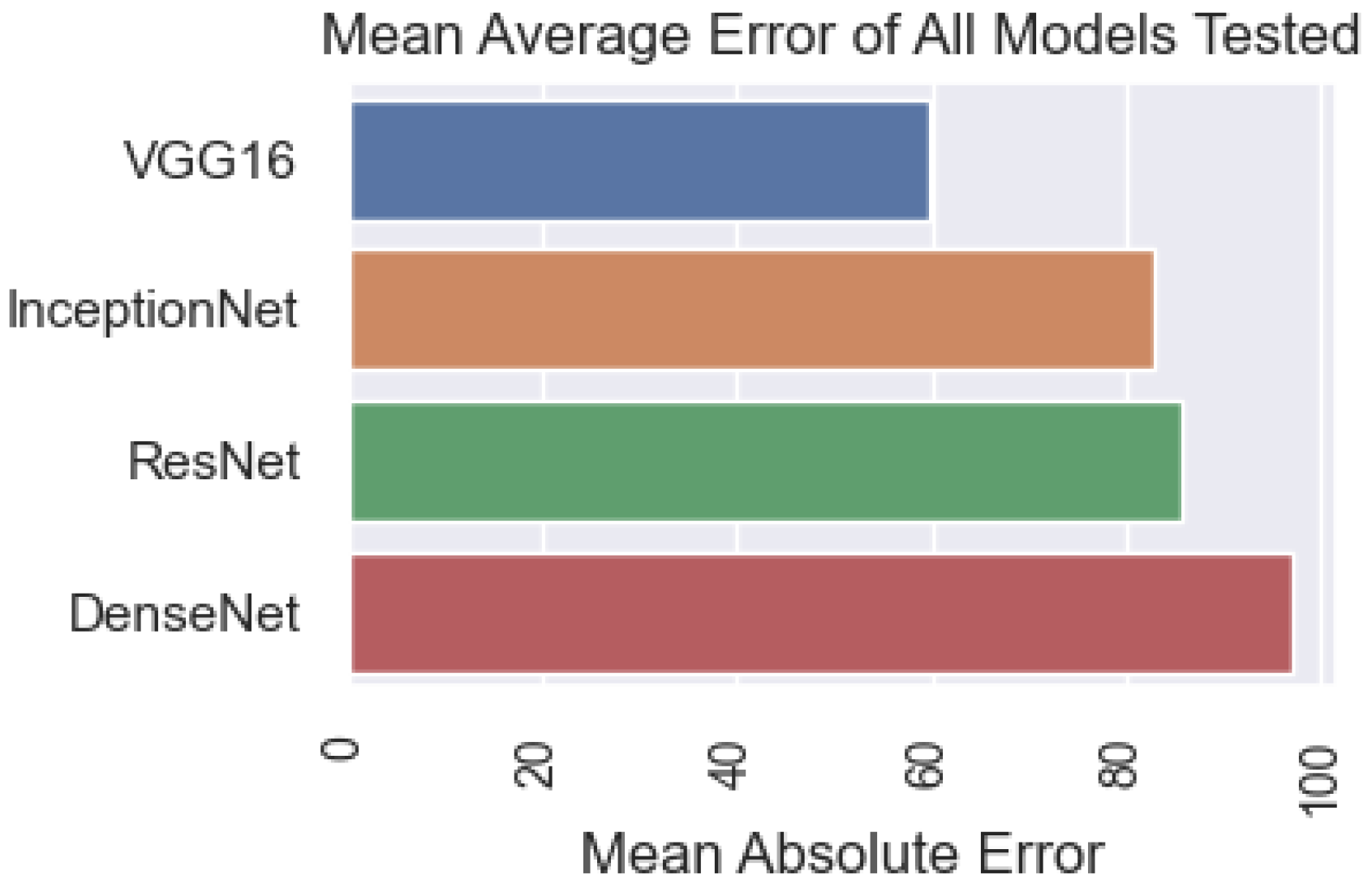
3. Results and Discussion
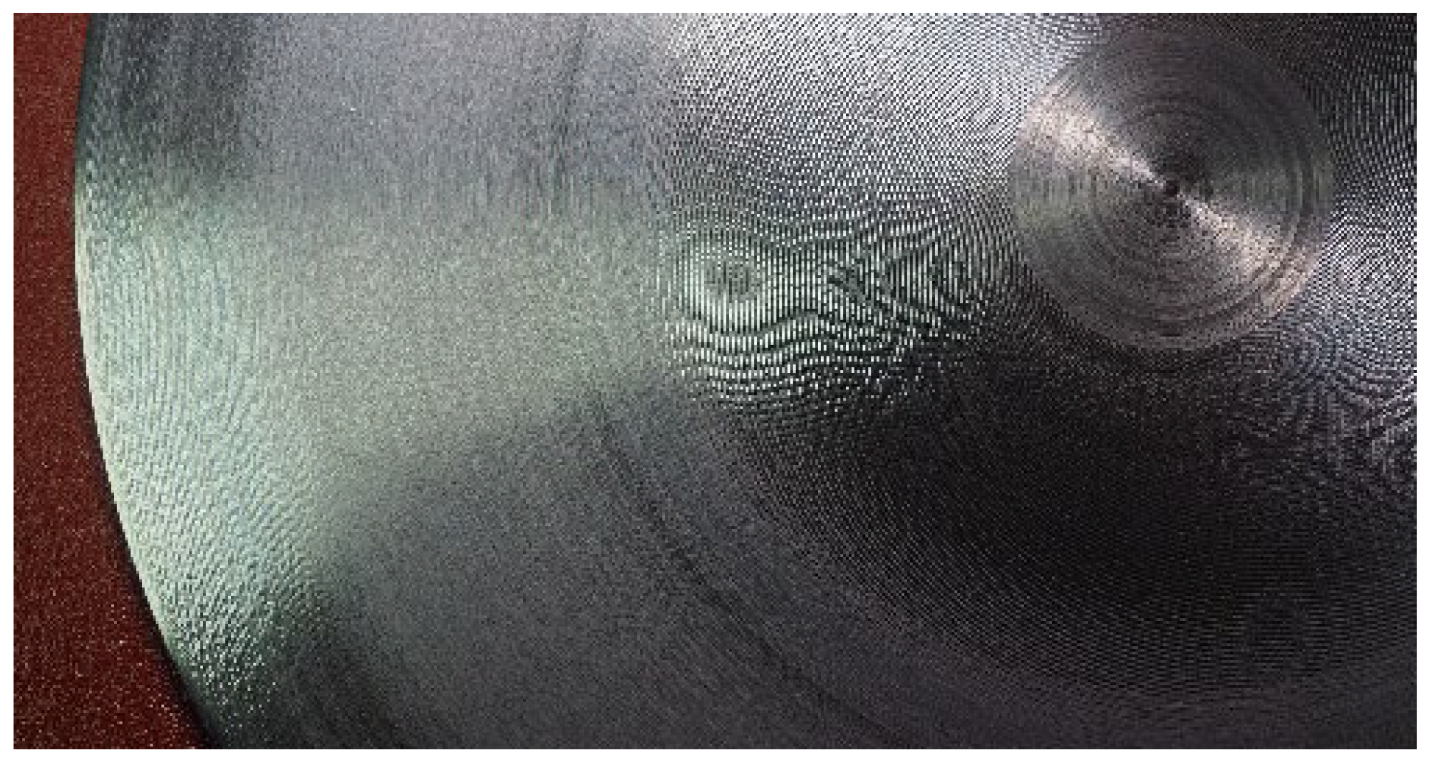
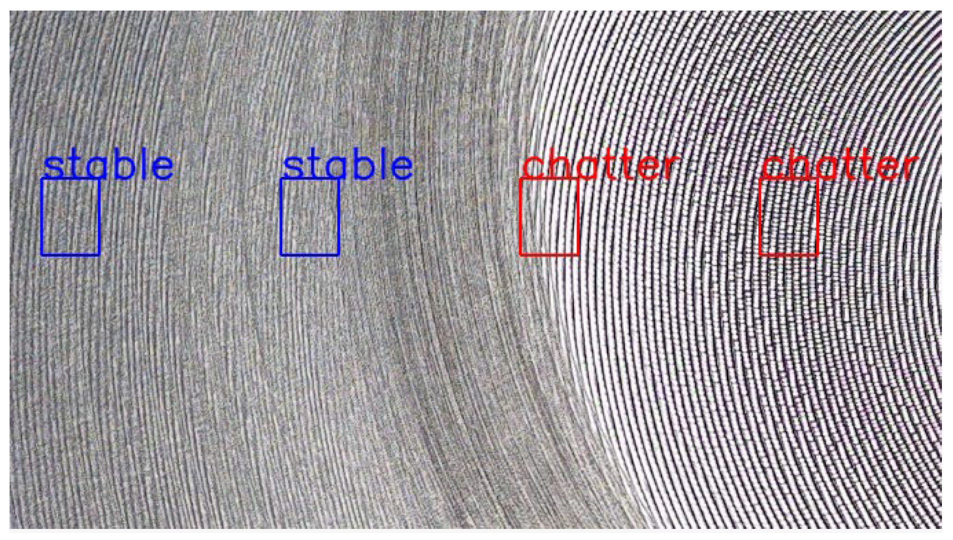
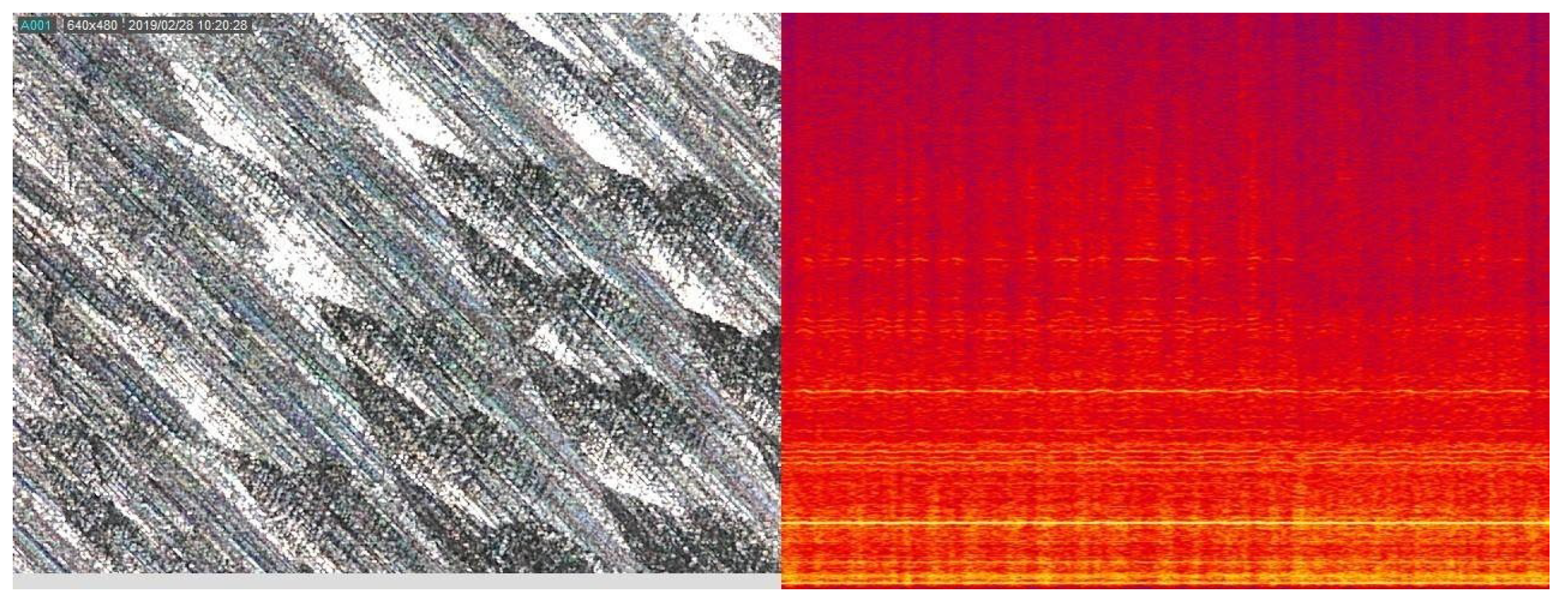
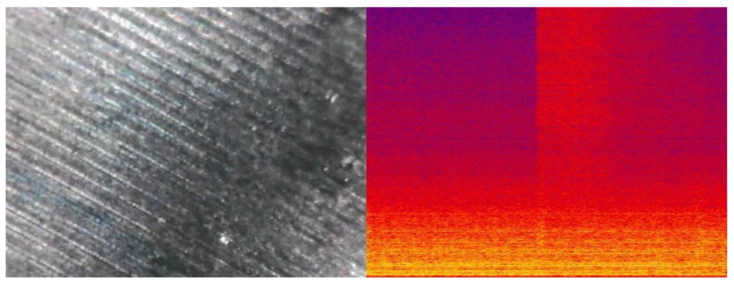
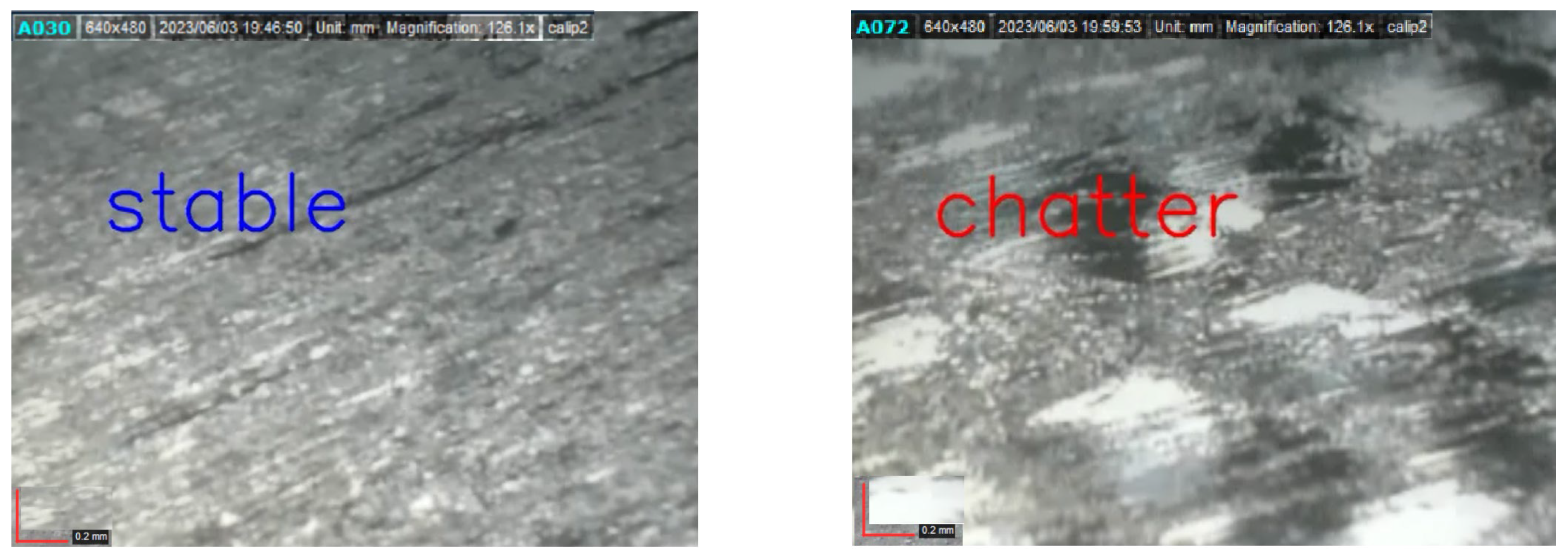
3.1. Data Collection and Processing
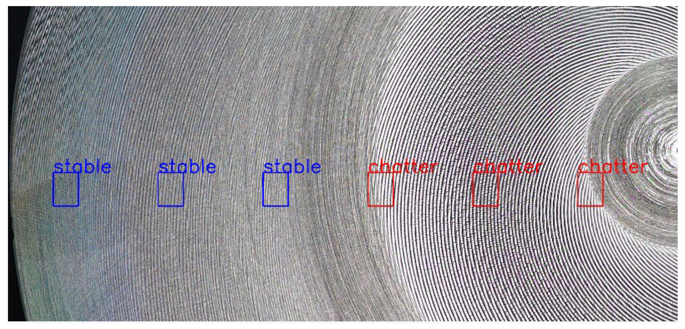
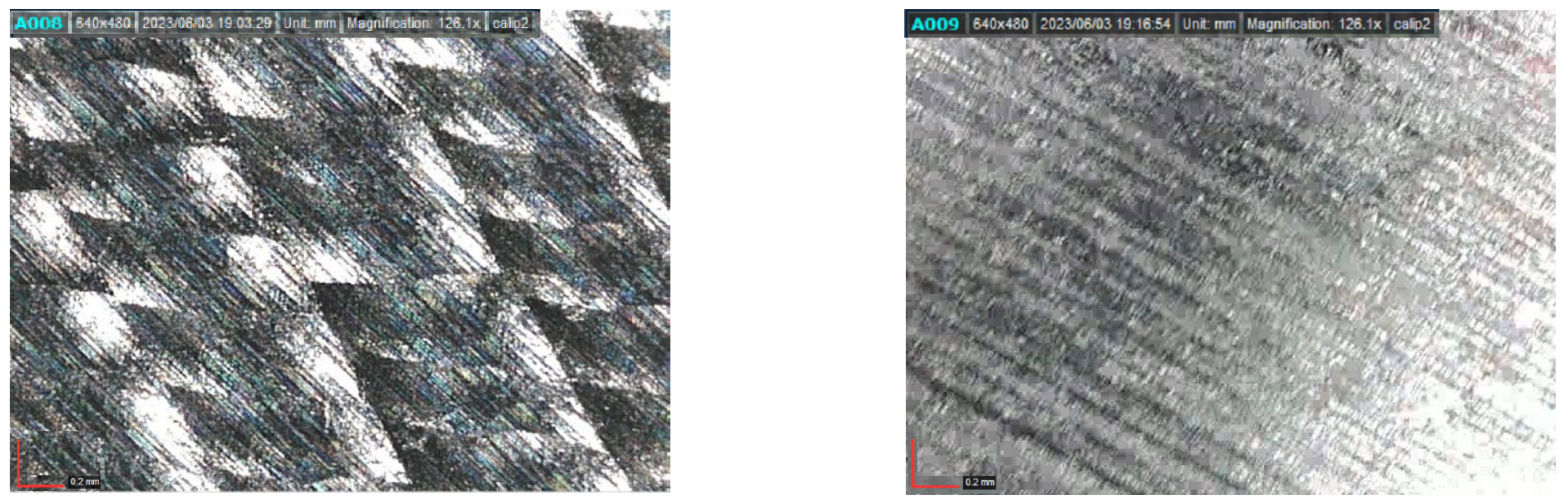
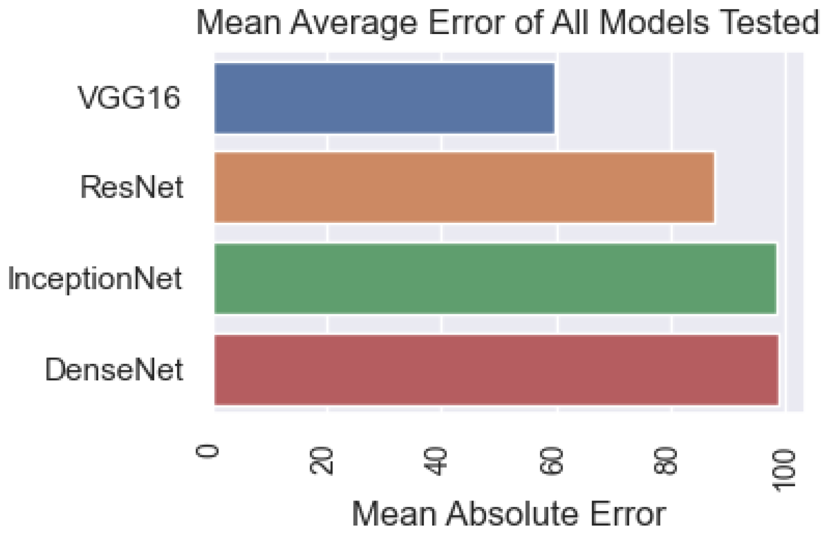
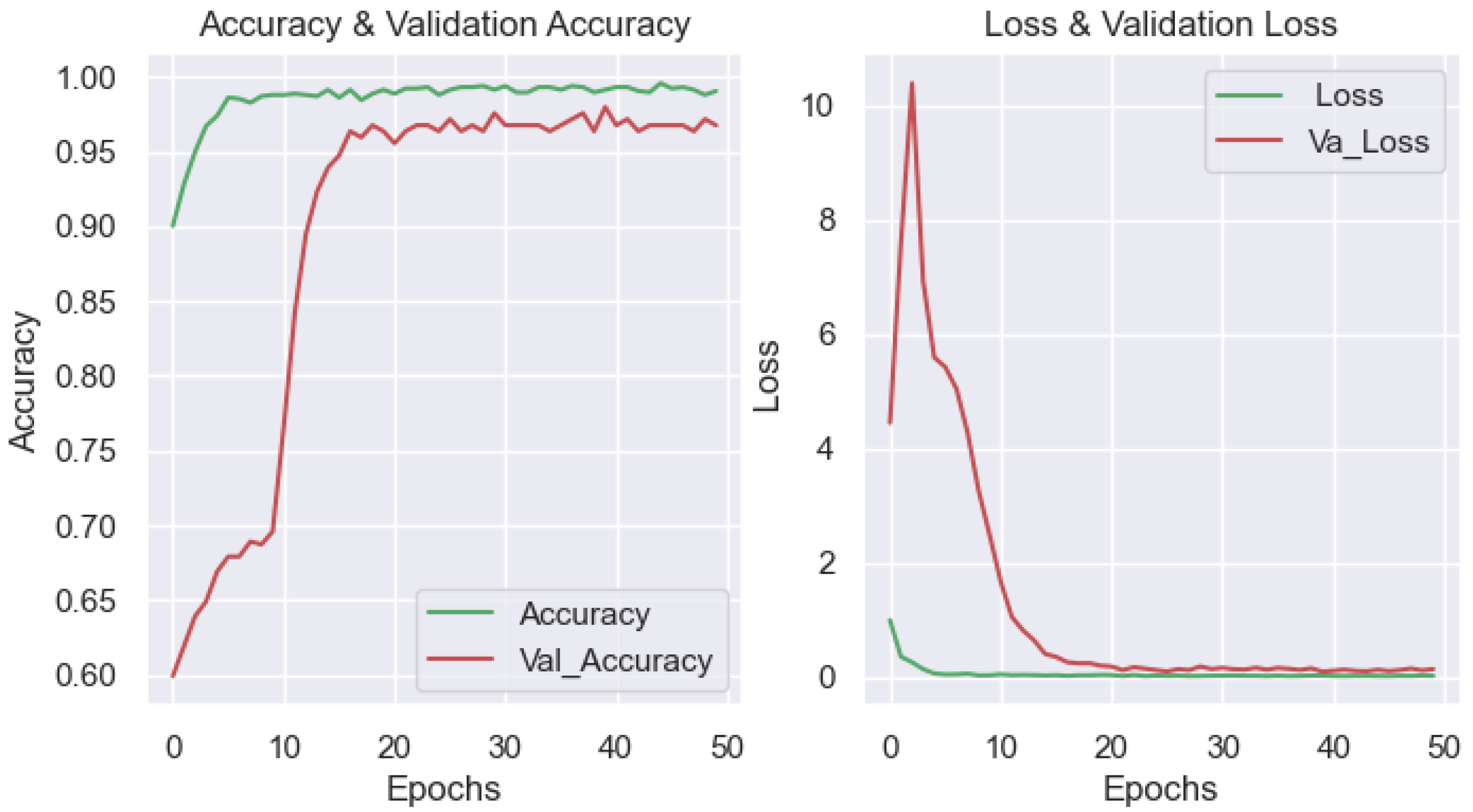
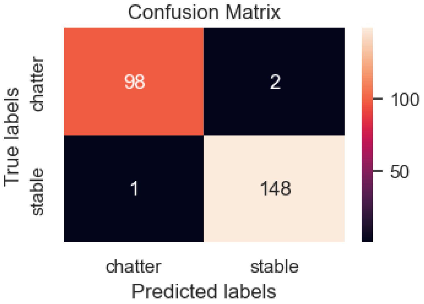
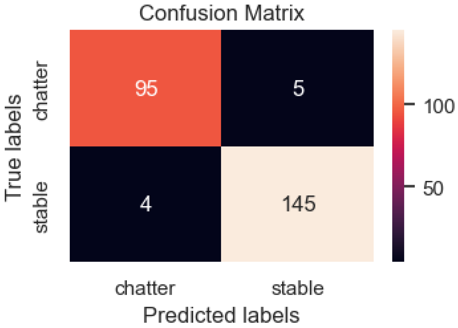
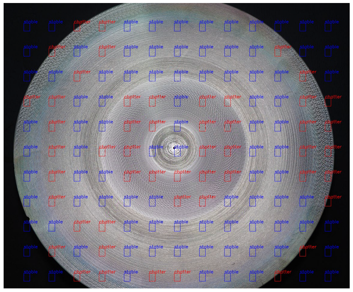
3.2. The Results of Applying CNN Models to Detect Chatter Using Surface Images of Parts during Turning
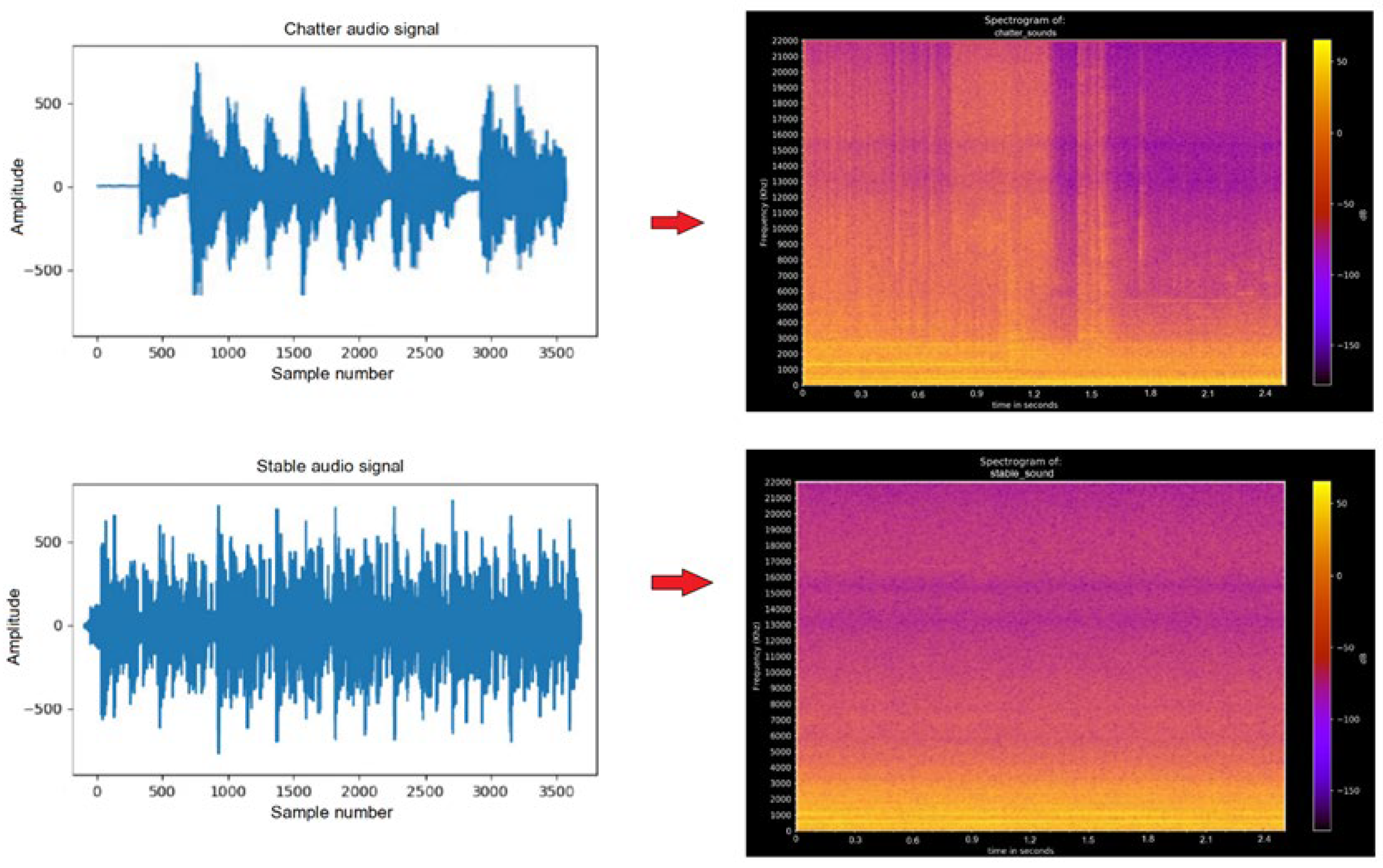
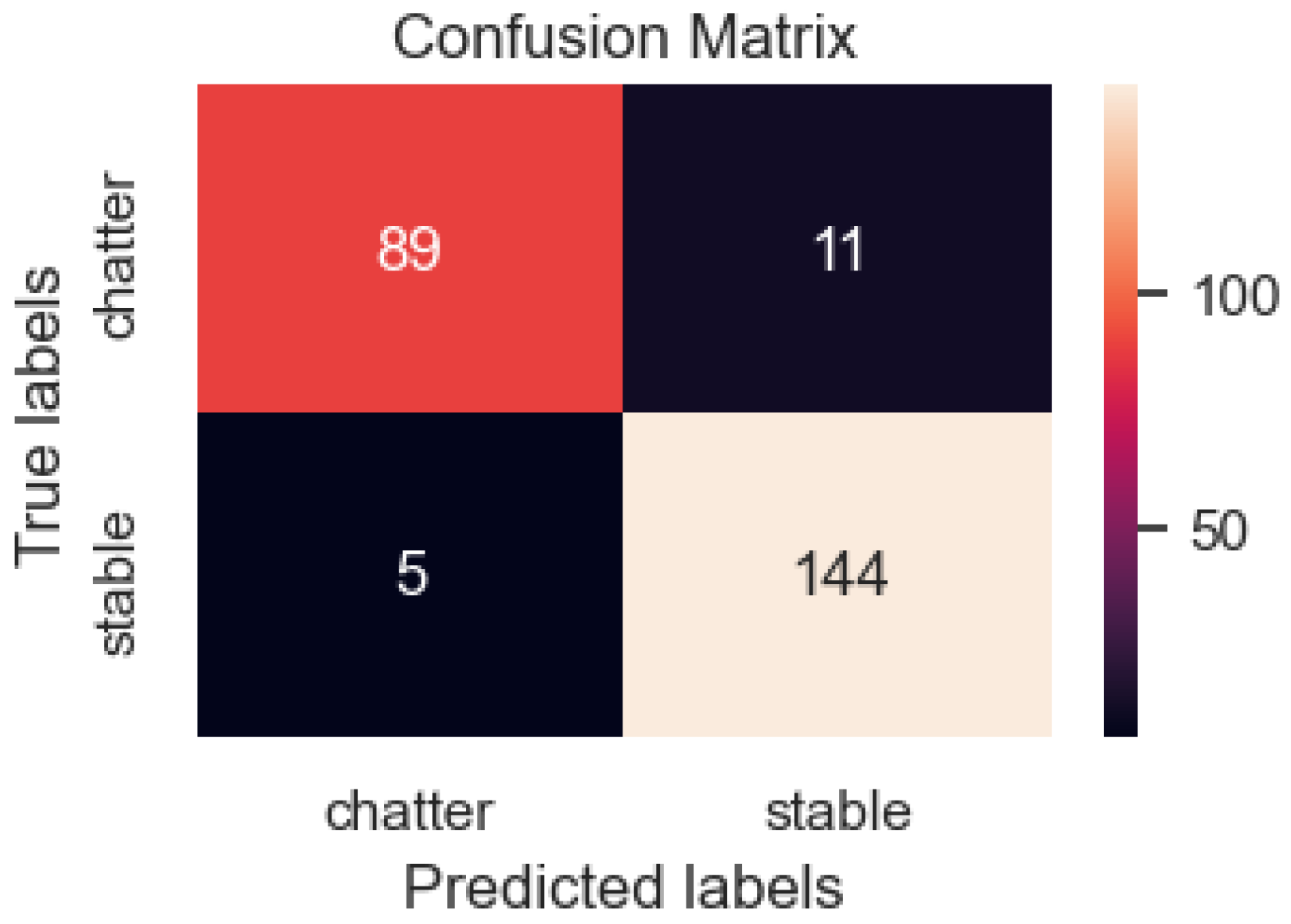
3.3. Results of Applying CNN Models to Detect Chatter by Acoustic Data during Turning
3.4. Model Results for Image Files Combined between Image and Sound Files
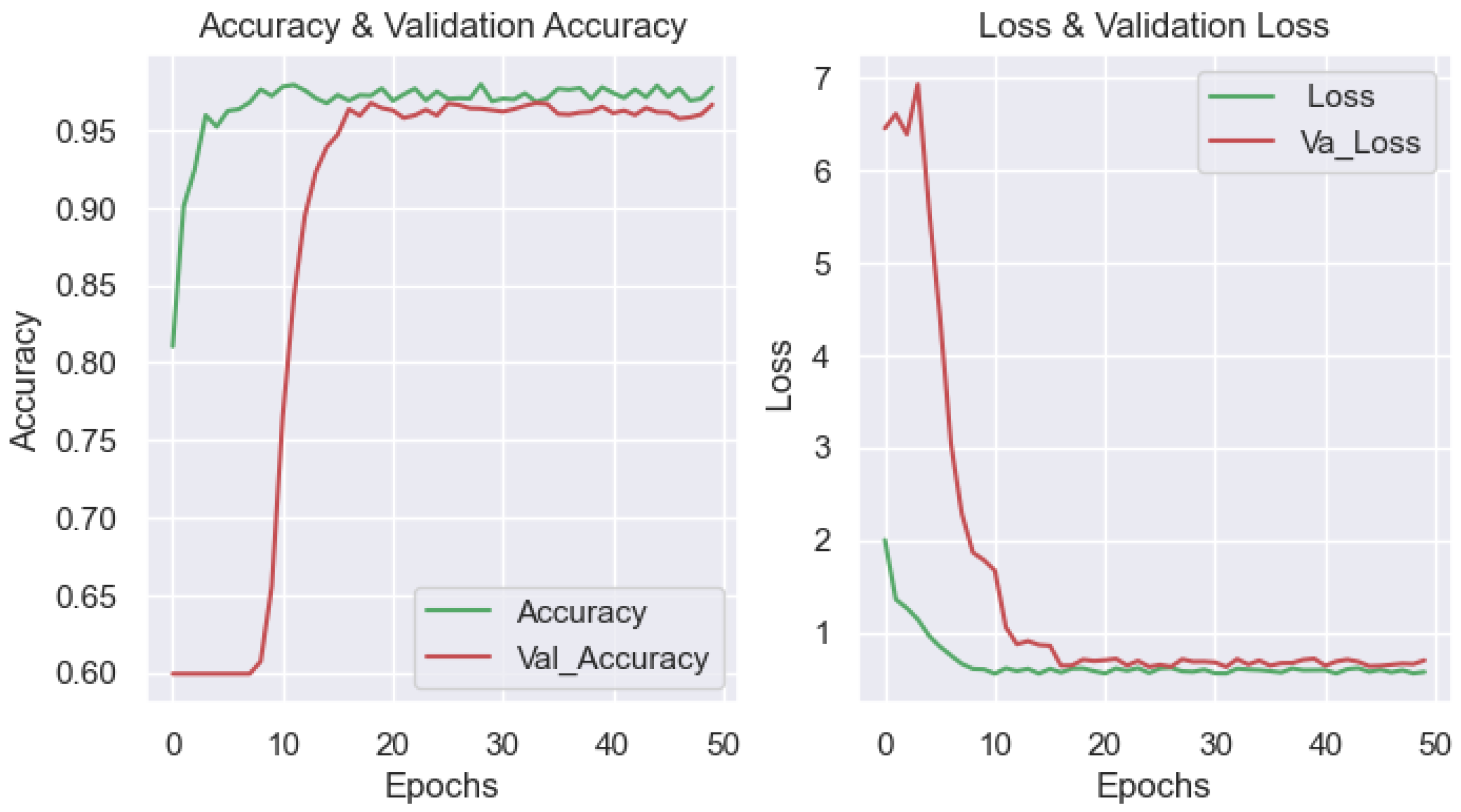
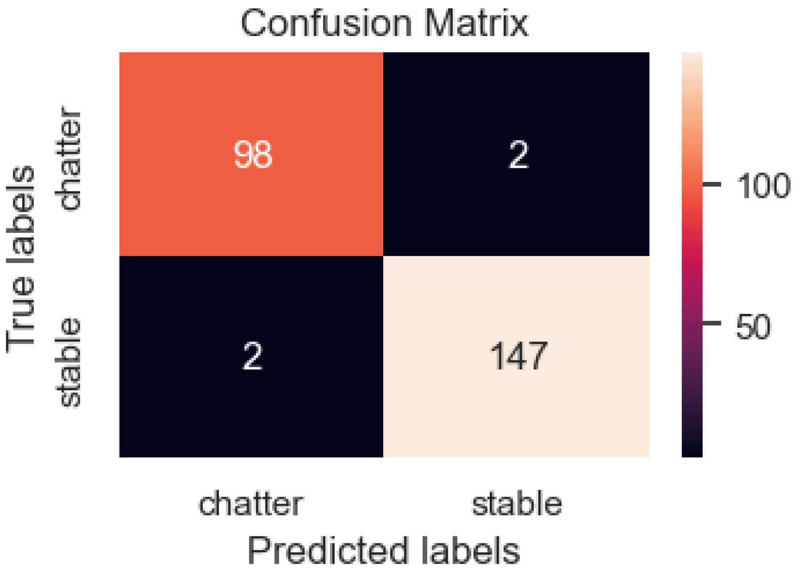
3.5. Model Results with Input Data of the Two-Input Model
3.6. Discussion
4. Conclusions
Author Contributions
Funding
Data Availability Statement
Acknowledgments
Conflicts of Interest
References
- Bravo, U.; Altuzarra, O.; De Lacalle, L.N.L.; Sánchez, J.A.; Campa, F.J. Stability limits of milling considering the flexibility of the workpiece and the machine. Int. J. Mach. Tools Manuf. 2005, 45, 1669–1680. [Google Scholar] [CrossRef]
- Altintaş, Y.; Budak, E. Analytical Prediction of Stability Lobes in Milling. CIRP Ann. 1995, 44, 357–362. [Google Scholar] [CrossRef]
- Urbikain, G.; Olvera, D.; López de Lacalle, L.N.; Beranoagirre, A.; Elías-Zuñiga, A. Prediction Methods and Experimental Techniques for Chatter Avoidance in Turning Systems: A Review. Appl. Sci. 2019, 9, 4718. [Google Scholar] [CrossRef] [Green Version]
- Dumanli, A.; Sencer, B. Active control of high frequency chatter with machine tool feed drives in turning. CIRP Ann. 2021, 70, 309–312. [Google Scholar] [CrossRef]
- Wan, S.; Li, X.; Su, W.; Yuan, J.; Hong, J.; Jin, X. Active damping of milling chatter vibration via a novel spindle system with an integrated electromagnetic actuator. Precis. Eng. 2019, 57, 203–210. [Google Scholar] [CrossRef]
- Fernández-Lucio, P.; Del Val, A.G.; Plaza, S.; Pereira, O.; Fernández-Valdivielso, A.; de Lacalle, L.N.L. Threading holder based on axial metal cylinder pins to reduce tap risk during reversion instant. Alex. Eng. J. 2023, 66, 845–859. [Google Scholar] [CrossRef]
- Rubio, L.; Loya, J.A.; Miguélez, M.H.; Fernández-Sáez, J. Optimization of passive vibration absorbers to reduce chatter in boring. Mech. Syst. Signal. Process. 2013, 41, 691–704. [Google Scholar] [CrossRef] [Green Version]
- Miguélez, M.H.; Rubio, L.; Loya, J.A.; Fernández-Sáez, J. Improvement of chatter stability in boring operations with passive vibration absorbers. Int. J. Mech. Sci. 2010, 52, 1376–1384. [Google Scholar] [CrossRef] [Green Version]
- Pelayo, G.U.; Trejo, D.O. Model-based phase shift optimization of serrated end mills: Minimizing forces and surface location error. Mech. Syst. Signal. Process. 2020, 144, 106860. [Google Scholar] [CrossRef]
- Urbikain, G.; Olvera, D.; de Lacalle, L.N.L.; Elías-Zúñiga, A. Spindle speed variation technique in turning operations: Modeling and real implementation. J. Sound. Vib. 2016, 383, 384–396. [Google Scholar] [CrossRef]
- Pelayo, G.U.; Olvera-Trejo, D.; Budak, E.; Wan, M. Special Issue on Machining systems and signal processing: Advancing machining processes through algorithms, sensors and devices. Mech. Syst. Signal. Process. 2023, 182, 109575. [Google Scholar] [CrossRef]
- Urbikain, G.; de Lacalle, L.N.L. MoniThor: A complete monitoring tool for machining data acquisition based on FPGA programming. SoftwareX 2020, 11, 100387. [Google Scholar] [CrossRef]
- Wu, S.; Li, R.; Liu, X.; Yang, L.; Zhu, M. Experimental study of thin wall milling chatter stability nonlinear criterion. Procedia CIRP 2016, 56, 422–427. [Google Scholar] [CrossRef] [Green Version]
- Dong, X.; Zhang, W. Chatter identification in milling of the thin-walled part based on complexity index. Int. J. Adv. Manuf. Technol. Technol. 2017, 91, 3327–3337. [Google Scholar] [CrossRef]
- Yamato, S.; Hirano, T.; Yamada, Y.; Koike, R.; Kakinuma, Y. Sensor-less online chatter detection in turning process based on phase monitoring using power factor theory. Precis. Eng. 2018, 51, 103–116. [Google Scholar] [CrossRef]
- Peng, C.; Wang, L.; Liao, T.W. A new method for the prediction of chatter stability lobes based on dynamic cutting force simulation model and support vector machine. J. Sound. Vib. 2015, 354, 118–131. [Google Scholar] [CrossRef]
- Grossi, N.; Sallese, L.; Scippa, A.; Campatelli, G. Chatter stability prediction in milling using speed-varying cutting force coefficients. Procedia CIRP 2014, 14, 170–175. [Google Scholar] [CrossRef] [Green Version]
- Filippov, A.V.; Nikonov, A.Y.; Rubtsov, V.E.; Dmitriev, A.I.; Tarasov, S.Y. Vibration and acoustic emission monitoring the stability of peakless tool turning: Experiment and modeling. J. Mater. Process. Technol. 2017, 246, 224–234. [Google Scholar] [CrossRef]
- Potočnik, P.; Thaler, T.; Govekar, E. Multisensory chatter detection in band sawing. Proc. CIRP 2013, 8, 469–474. [Google Scholar] [CrossRef] [Green Version]
- Cao, H.; Yue, Y.; Chen, X.; Zhang, X. Chatter detection in milling process based on synchro squeezing transform of sound signals. Int. J. Adv. Manuf. Technol. 2017, 89, 2747–2755. [Google Scholar] [CrossRef]
- Sallese, L.; Grossi, N.; Scippa, A.; Campatelli, G. Investigation and correction of actual microphone response for chatter detection in milling operations. Meas. Control. 2017, 50, 45–52. [Google Scholar] [CrossRef]
- Chaudhary, S.; Taran, S.; Bajaj, V.; Sengur, A. Convolutional neural network based approach towards motor imagery tasks EEG signals classification. IEEE Sens. J. 2019, 19, 4494–4500. [Google Scholar] [CrossRef]
- Ho, Q.N.T.; Do, T.T.; Minh, P.S. Studying the Factors Affecting Tool Vibration and Surface Quality during Turning through 3D Cutting Simulation and Machine Learning Model. Micromachines 2023, 14, 1025. [Google Scholar] [CrossRef]
- Checa, D.; Urbikain, G.; Beranoagirre, A.; Bustillo, A.; de Lacalle, L.N.L. Using Machine-Learning techniques and Virtual Reality to design cutting tools for energy optimization in milling operations. Int. J. Comput. Integr. Manuf. 2022, 35, 951–971. [Google Scholar] [CrossRef]
- Ma, M.; Liu, L.; Chen, Y.A. KM-Net Model Based on k-Means Weight Initialization for Images Classification. In Proceedings of the 2018 IEEE 20th International Conference on High Performance Computing and Communications, IEEE 16th International Conference on Smart City, IEEE 4th International Conference on Data Science and Systems (HPCC/SmartCity/DSS), Exeter, UK, 28–30 June 2018; pp. 1125–1128. [Google Scholar] [CrossRef]
- Zheng, M.; Tang, W.; Zhao, X. Hyperparameter optimization of neural network-driven spatial models accelerated using cyberenabled high-performance computing. Int. J. Geogr. Inf. Sci. 2019, 33, 314–345. [Google Scholar] [CrossRef]
- Simonyan, K.; Zisserman, A. Very Deep Convolutional Networks for Large-Scale Image Recognition. arXiv 2014, arXiv:1409.1556. [Google Scholar] [CrossRef]
- Huang, G.; Liu, Z.; van der Maaten, L.; Weinberger, K.Q. Densely Connected Convolutional Networks. arXiv 2018, arXiv:1608.06993. [Google Scholar] [CrossRef]
- He, K.; Zhang, X.; Ren, S.; Sun, J. Deep Residual Learning for Image Recognition. arXiv 2015, arXiv:1512.03385. [Google Scholar] [CrossRef]
- Szegedy, C.; Liu, W.; Jia, Y.; Sermanet, P.; Reed, S.; Anguelov, D.; Erhan, D.; Vanhoucke, V.; Rabinovich, A. Going Deeper with Convolutions. arXiv 2014, arXiv:1409.4842. [Google Scholar] [CrossRef]
- Zhu, W.; Zhuang, J.; Guo, B.; Teng, W.; Wu, F. An optimized convolutional neural network for chatter detection in the milling of thin-walled parts. Int. J. Adv. Manuf. Technol. 2020, 106, 3881–3895. [Google Scholar] [CrossRef]
- Tran, M.-Q.; Liu, M.-K.; Tran, Q.-V. Milling chatter detection using scalogram and deep convolutional neural network. Int. J. Adv. Manuf. Technol. 2020, 107, 1505–1516. [Google Scholar] [CrossRef]
- Rahimi, M.H.; Huynh, H.N.; Altintas, Y. Online chatter detection in milling with hybrid machine learning and physics-based model. CIRP J. Manuf. Sci. Technol. 2021, 35, 25–40. [Google Scholar] [CrossRef]
- Sener, B.; Gudelek, M.U.; Ozbayoglu, A.M.; Unver, H.O. A novel chatter detection method for milling using deep convolution neural networks. Measurement 2021, 182, 109689. [Google Scholar] [CrossRef]
- Kounta, C.A.K.A.; Arnaud, L.; Kamsu-Foguem, B.; Tangara, F. Deep learning for the detection of machining vibration chatter. Adv. Eng. Softw. 2023, 180, 103445. [Google Scholar] [CrossRef]


| Parameters | Values | |
|---|---|---|
| Workpiece | Material Diameter Thickness | SS_400 220 mm 15 mm |
| Tool | Material Rake angle Relief angle Cutting edge radius Tool holder length | Carbide 5° 10° 0.2 mm 50 mm |
| Cutting | Velocity spindle Feed rate Depth of cut (DOC) | 800 rev/min 0.1 mm/rev 2 mm |
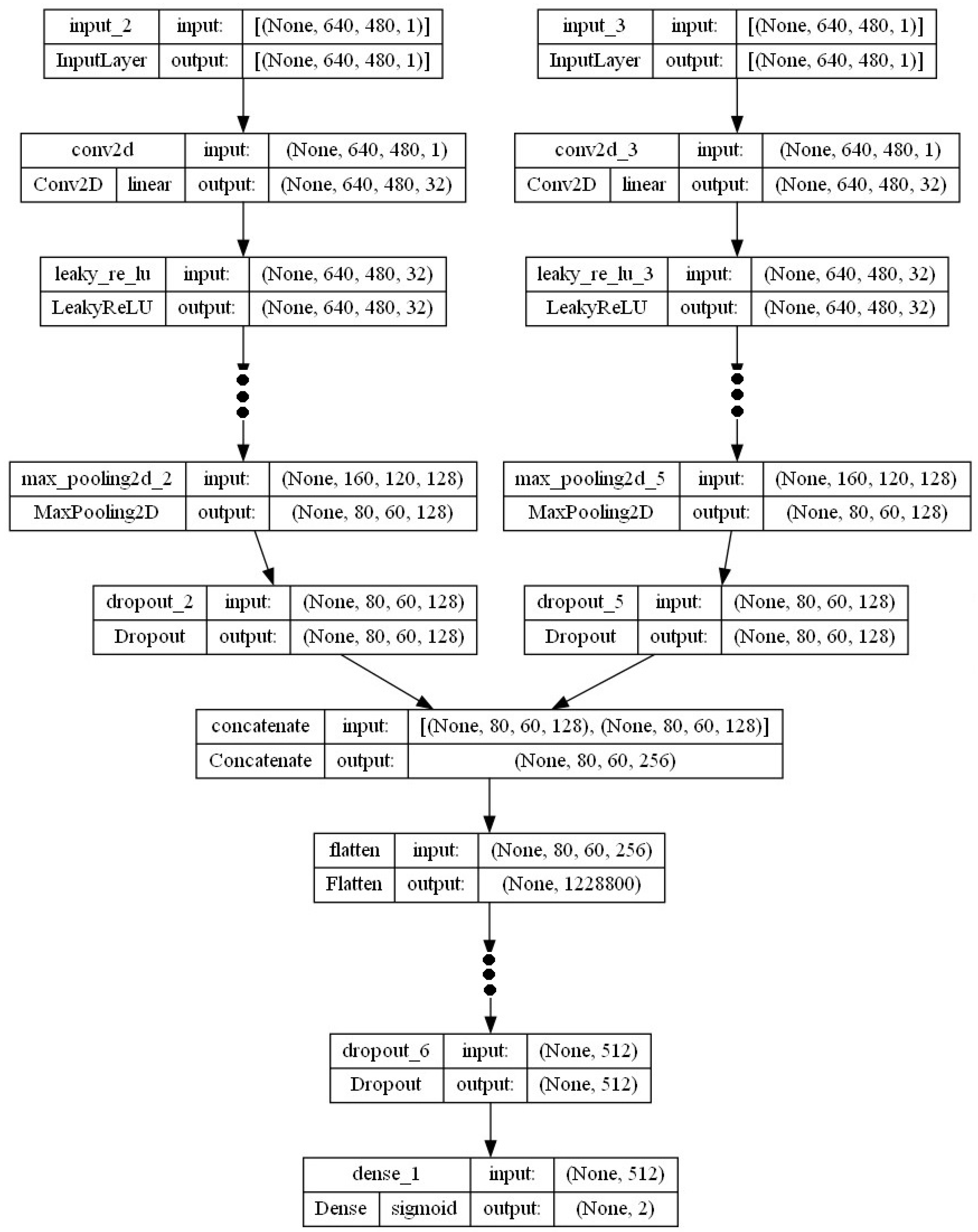
| Layer (Type) | Output Shape Param # | Connected to |
|---|---|---|
| input_2 (InputLayer) | [(None, 640, 480, 1 0)] | [] |
| input_3 (InputLayer) | [(None, 640, 480, 1 0)] | [] |
| conv2d (Conv2D) | (None, 640, 480, 32 320) | [‘input_2[0][0]’] |
| conv2d_3 (Conv2D) | (None, 640, 480, 32 320) | [‘input_3[0][0]’] |
| leaky_re_lu (LeakyReLU) | (None, 640, 480, 32 0) | [‘conv2d [0][0]’] |
| leaky_re_lu_3 (LeakyReLU) | (None, 640, 480, 32 0) | [‘conv2d_3[0][0]’] |
| max_pooling2d (MaxPooling2D) | (None, 320, 240, 32 0) | [‘leaky_re_lu[0][0]’] |
| max_pooling2d_3 (MaxPooling2D) | (None, 320, 240, 32 0) | [‘leaky_re_lu_3[0][0]’] |
| dropout (Dropout) | (None, 320, 240, 32 0) | [‘max_pooling2d[0][0]’] |
| dropout_3 (Dropout) | (None, 320, 240, 32 0) | [‘max_pooling2d_3[0][0]’] |
| conv2d_1 (Conv2D) | (None, 320, 240, 64 18496) | [‘dropout[0][0]’] |
| conv2d_4 (Conv2D) | (None, 320, 240, 64 18496) | [‘dropout_3[0][0]’] |
| leaky_re_lu_1 (LeakyReLU) | (None, 320, 240, 64 0) | [‘conv2d_1[0][0]’] |
| leaky_re_lu_4 (LeakyReLU) | (None, 320, 240, 64 0) | [‘conv2d_4[0][0]’] |
| max_pooling2d_1 (MaxPooling2D) | (None, 160, 120, 64 0) | [‘leaky_re_lu_1[0][0]’] |
| max_pooling2d_4 (MaxPooling2D) | (None, 160, 120, 64 0) | [‘leaky_re_lu_4[0][0]’] |
| dropout_1 (Dropout) | (None, 160, 120, 64 0) | [‘max_pooling2d_1[0][0]’] |
| dropout_4 (Dropout) | (None, 160, 120, 64 0) | [‘max_pooling2d_4[0][0]’] |
| conv2d_2 (Conv2D) | (None, 160, 120, 12 738568) | [‘dropout_1[0][0]’] |
| conv2d_5 (Conv2D) | (None, 160, 120, 12 738568) | [‘dropout_4[0][0]’] |
| leaky_re_lu_2 (LeakyReLU) | (None, 160, 120, 12 08) | [‘conv2d_2[0][0]’] |
| leaky_re_lu_5 (LeakyReLU) | (None, 160, 120, 12 08) | [‘conv2d_5[0][0]’] |
| max_pooling2d_2 (MaxPooling2D) | (None, 80, 60, 128) 0 | [‘leaky_re_lu_2[0][0]’] |
| max_pooling2d_5 (MaxPooling2D) | (None, 80, 60, 128) 0 | [‘leaky_re_lu_5[0][0]’] |
| dropout_2 (Dropout) | (None, 80, 60, 128) 0 | [‘max_pooling2d_2[0][0]’] |
| dropout_5 (Dropout) | (None, 80, 60, 128) 0 | [‘max_pooling2d_5[0][0]’] |
| concatenate (Concatenate) | (None, 80, 60, 256) 0 | [‘dropout_2[0][0]’, |
| flatten (Flatten) | (None, 1228800) 0 | [‘concatenate[0][0]’] |
| dense (Dense) | (None,512)62914612 | [‘flatten[0][0]’] |
| leaky_re_lu_6 (LeakyReLU) | (None, 512) 0 | [‘dense[0][0]’] |
| dropout_6 (Dropout) | (None, 512) 0 | [‘leaky_re_lu_6[0][0]’] |
| dense_1 (Dense) | (None, 2) 1026 | [‘dropout_6[0][0]’] |
| Total params: 629,332,482 | ||
| Trainable params: 629,332,482 |
| Hyperparameter | Value |
|---|---|
| Batch size | 32 |
| Optimizer | Adam |
| learning rate | ReduceLROnPlateau |
| Loss | categorical_crossentropy |
| Epochs | 50 |
| Data | Train (80%) | Valid (10%) | Test (10%) | Total (100%) | Labels |
|---|---|---|---|---|---|
| Images | 464 | 99 | 100 | 663 | chatter |
| 690 | 148 | 149 | 987 | stable | |
| Sounds | 464 | 99 | 100 | 663 | chatter |
| 690 | 148 | 149 | 987 | stable | |
| Combine image_sound | 464 | 99 | 100 | 663 | chatter |
| 690 | 148 | 149 | 987 | stable |
| Chatter (Class 0) | Stable (Class 1) | Accuracy | Macro Avg | Weighted Avg | |
|---|---|---|---|---|---|
| precision | 0.989899 | 0.986667 | 0.987952 | 0.988283 | 0.987965 |
| recall | 0.980000 | 0.993289 | 0.987952 | 0.986644 | 0.987952 |
| f1-score | 0.984925 | 0.989967 | 0.987952 | 0.987446 | 0.987942 |
| support | 100 | 149 | 0.987952 | 249 | 249 |
| Chatter (Class 0) | Stable (Class 1) | Accuracy | Macro Avg | Weighted Avg | |
|---|---|---|---|---|---|
| precision | 0.946809 | 0.929032 | 0.935743 | 0.937920 | 0.936171 |
| recall | 0.890000 | 0.966443 | 0.935743 | 0.928221 | 0.935743 |
| f1-score | 0.917526 | 0.947368 | 0.935743 | 0.932447 | 0.935383 |
| support | 100 | 149 | 0.935743 | 249 | 249 |
| Chatter (Class 0) | Stable (Class 1) | Accuracy | Macro Avg | Weighted Avg | |
|---|---|---|---|---|---|
| precision | 0.959596 | 0.966667 | 0.963855 | 0.963131 | 0.963827 |
| recall | 0.950000 | 0.973154 | 0.963855 | 0.961577 | 0.963855 |
| f1-score | 0.954774 | 0.969900 | 0.963855 | 0.962337 | 0.963825 |
| support | 100 | 149 | 0.963855 | 249 | 249 |
| Chatter (Class 0) | Stable (Class 1) | Accuracy | Macro Avg | Weighted Avg | |
|---|---|---|---|---|---|
| Precision | 0.98 | 0.986577 | 0.983936 | 0.983289 | 0.983936 |
| Recall | 0.98 | 0.986577 | 0.983936 | 0.983289 | 0.983936 |
| f1-score | 0.98 | 0.986577 | 0.983936 | 0.983289 | 0.983936 |
| Support | 100 | 149 | 0.983936 | 249 | 249 |
| Input | Model | Precision | Recall | F1_Score |
|---|---|---|---|---|
| Image | DenseNet | 0.99 | 0.98 | 0.98 |
| Sound | DenseNet | 0.95 | 0.89 | 0.92 |
| Combine image and sound | DenseNet | 0.96 | 0.95 | 0.95 |
| Image, Sound | Two inputs model | 0.98 | 0.96 | 0.97 |
| REF. | Author | Pretreatment | Input Data | Classification | Precision |
|---|---|---|---|---|---|
| This paper | FFT, Size Reduction | Images and sounds | Binary | 98% | |
| [31] | (W. Zhu et al., 2020) | Size reduction | Images | Binary | 98.26% |
| [32] | (Tran et al., 2020) | CWT | Images | Multilabel | 99.67% |
| [33] | (Rahimi et al., 2021) | STFT | Images | Multilabel | 98.90% |
| [34] | (Sener et al., 2021) | CWT | Images—cutting parameters | Multilabel | 99.8% |
| [35] | (C. Kounta et al., 2023) | FFT | Sound cutting | Multilabel | 99.71% |
Disclaimer/Publisher’s Note: The statements, opinions and data contained in all publications are solely those of the individual author(s) and contributor(s) and not of MDPI and/or the editor(s). MDPI and/or the editor(s) disclaim responsibility for any injury to people or property resulting from any ideas, methods, instructions or products referred to in the content. |
© 2023 by the authors. Licensee MDPI, Basel, Switzerland. This article is an open access article distributed under the terms and conditions of the Creative Commons Attribution (CC BY) license (https://creativecommons.org/licenses/by/4.0/).
Share and Cite
The Ho, Q.N.; Do, T.T.; Minh, P.S.; Nguyen, V.-T.; Nguyen, V.T.T. Turning Chatter Detection Using a Multi-Input Convolutional Neural Network via Image and Sound Signal. Machines 2023, 11, 644. https://doi.org/10.3390/machines11060644
The Ho QN, Do TT, Minh PS, Nguyen V-T, Nguyen VTT. Turning Chatter Detection Using a Multi-Input Convolutional Neural Network via Image and Sound Signal. Machines. 2023; 11(6):644. https://doi.org/10.3390/machines11060644
Chicago/Turabian StyleThe Ho, Quang Ngoc, Thanh Trung Do, Pham Son Minh, Van-Thuc Nguyen, and Van Thanh Tien Nguyen. 2023. "Turning Chatter Detection Using a Multi-Input Convolutional Neural Network via Image and Sound Signal" Machines 11, no. 6: 644. https://doi.org/10.3390/machines11060644