Intelligent Position Controller for Unmanned Aerial Vehicles (UAV) Based on Supervised Deep Learning

Abstract

In recent years, multi-rotor UAVs have become valuable tools in several productive fields, from entertainment to agriculture and security. However, during their flight trajectory, they sometimes do not accurately perform a specific set of tasks, and the implementation of flight controllers in these vehicles is required to achieve a successful performance. Therefore, this research describes the design of a flight position controller based on Deep Neural Networks and subsequent implementation for a multi-rotor UAV. Five promising Neural Network architectures are developed based on a thorough literature review, incorporating LSTM, 1-D convolutional, pooling, and fully-connected layers. A dataset is then constructed using the performance data of a PID flight controller, encompassing diverse trajectories with transient and steady-state information such as position, speed, acceleration, and motor output signals. The tuning of hyperparameters for each type of architecture is performed by applying the Hyperband algorithm. The best model obtained (LSTMCNN) consists of a combination of LSTM and CNN layers in one dimension. This architecture is compared with the PID flight controller in different scenarios employing evaluation metrics such as rise time, overshoot, steady-state error, and control effort. The findings reveal that our best models demonstrate the successful generalization of flight control tasks. While our best model is able to work with a wider operational range than the PID controller and offers step responses in the Y and X axis with $97\%$ and $98\%$ similarity, respectively, within the PID’s operational range. This outcome opens up possibilities for efficient online training of flight controllers based on Neural Networks, enabling the development of adaptable controllers tailored to specific application domains.

1. Introduction

Unmanned aerial vehicles (UAVs), commonly known as drones, have been around since the First World War and were initially used in the military field [1]. However, they are currently used for both civilian and commercial purposes as well [2]. Search and rescue operations [3], remote sensing [4], last-mile deliveries [5], and aerial spray and disinfection [6] are just a few practical applications.

Quadrotors are a type of six-degree-of-freedom (6-DOF) UAV with four rotors, which produce lift through difference in the thrust of the rotation of its propellers. Due to their vertical takeoff and landing (VTOL) capability, omnidirectional flight, and mobility in constrained spaces, UAV quadrotors can perform outdoor and indoor tasks. Furthermore, the lightweight, small size, versatility, easy handling, and low cost of quadrotors make them more suitable compared to the fixed-wing UAVs for short-term missions [7].

Disturbances such as wind, temperature, air pressure, reference changes, aerodynamic effects (ground effect, drag, and downwash), or uncertainties can cause the UAV to become unstable and get damaged, as the applications are designed for specific operating conditions [8]. To achieve the variety of intended applications, controllers must ensure stability, correct execution of movements in a short time with a small margin error, robustness, and efficient energy consumption [9]. However, the design of attitude and position controllers for quadrotors is challenging due to their unstable and under-acted nature and coupled and multi-variable nonlinear dynamics.

Several approaches have been developed to overcome the challenge of controlling quadrotor UAVs under different operating conditions. These approaches can be broadly categorized into model-based and model-free controllers. Model-based controllers require a precise understanding of the system and depend on a model. PID controller plus Linear-Quadratic Regulator (PID+LQR) [10] or robust Sliding Mode Control (SMC) [11] are examples of model-based controllers. However, these types of control approaches can be sensitive to modeling errors, and it is important to count on accurate modeling and system identification for effective control design [12].

A linear model for a nonlinear system can be obtained by using a small-signal approximation around an operating point [13]. These models allow the development of classical linear [14] and optimal [10] control systems, demonstrating stability even in environments with wind speed fluctuation [15]. In contrast, linear control algorithms fail to control the UAV in states other than the operating point.

More complex control systems have been proposed to improve the performance of UAVs under specific operation points and to enhance the stability of these vehicles in the presence of external disturbances, such as those considering the dependency between movement and attitude in our plant to offer a robust control in the presence of loads [16], un-modeled high-frequency dynamics [17], an adaptive control for multi-quadrotor cooperation under load uncertainties [18], Robust adaptive control for heterogeneous multi-quadrotor cooperation [19], and Adaptive Backstepping Control to deal with uncertainties and non-linear dynamics from the UAV model [20]. However, these models often require an accurate high-order mathematical model with sophisticated coefficient computations. Finally, although these approaches propose to solve specific points of operation un-modeled dynamic factors can lead to system instability, low convergence rate, chattering effect, or transient and steady-state problems.

Model-free controllers such as PD Hybrid Artificial Neural Network (PD-ANN) [21], Fuzzy Based Backstepping Control [22], and Nonlinear Integral Backstepping Model-free Control (NIB-MFC) [23] have been proposed to control under system uncertainties and modeling errors, resulting in a significant improvement in low-level control for UAVs compared to classical controllers [24]. Furthermore, intelligent models based on neural networks can generalize experience from provided data for different operating points, making them suitable for controlling and modeling complex dynamic systems such as UAV low-level control [25].

Model-free controllers can be further divided into online and offline approaches. Online methods such as Reinforcement Learning [26] build the data simultaneously as it is experienced but requires a lot of time and a high computational cost. Offline approaches [27] learn from a specified dataset and are faster and more efficient than online methods. Still, model performance depends on the quality and quantity of the available data. Combining both strategies, as proposed by Ashvin Nair and co. [28], can accelerate model learning by offline learning on a prior dataset and then fine-tuning with online interaction.

This paper is organized as follows: In Section 2, we describe the recent research effort in flight control systems toward intelligent control, robust control, hybrid approaches, and the paper’s contribution. Then, Section 3 explains the applied software and techniques proposed with definitions from the literature. Next, the results of the experiments used to evaluate our trained controllers and their evaluation compared to our base PID controller are explained in Section 4 and commented on in Section 5. Finally, the conclusions and recommendations for future works are commented on in Section 6 and Section 7.

2. Related Works

The UAV control area has been widely explored by applying a wide variety of control techniques and approaches, such as linear and non-linear control, robust and adaptive control, machine learning, and reinforcement learning, among many more.

2.1. Linear Controllers

The proportional–integral–derivative controller (PID) is the most popular control technique used for industrial drones due to its ease of implementation and reliability [29]. Some research aims to find the best combination of constants applied to a UAV, such as the Ziegler–Nichols technique used in a closed-loop to determine stability limits and PID constants [30], and the application of bio-inspired searching algorithms to find the best parameters for the PID controller [31]. More complex approaches include PID+LQR [10] or LQ and H${}_{\infty }$ [15]. It is worth pointing out that these controllers provide the basic functionalities of flight control even in the presence of environmental changes such as wind direction [15].

2.2. Non-Linear and Robust Control Techniques

Linear control techniques have limitations when the control action is far from its equilibrium point. Researchers have attempted to solve these problems by using non-linear or robust control techniques. For example, Lyapunov techniques [32] and [33], Fuzzy based [34], Backstepping control [35], and Geometric Control [36]. These developments are more robust in challenging environmental conditions. However, for our study, on the one hand, implementing these techniques requires a thorough understanding of system uncertainties, system models, and robust control theory [37]. On the other hand, these control techniques are dependent on an accurate model, but most of the proposed models do not abstract operation points of drones with high attitude angles [38]. Therefore, mismatches in the approximated model for our UAVs could lead to instability and singularities when complex rotational trajectories are required with these controllers.

2.3. Machine Learning Techniques

According to [39], machine learning techniques offer potential solutions to develop a versatile controller for a UAV with variable parameters in its environment. Ref. [40] found that an intelligent flight assistant based on the simplest neural network architecture has the capacity to outperform human flight performance. Refs. [41,42] designed robust and efficient controllers with an auto-tuning feature. In [43], they implemented an adaptable state observer based on a neural network, which updates the error states dynamically, offering a notable performance even when the measures contain noise. Further, ref. [44] developed a controller by applying the actor–critic method with a deterministic policy gradient, whereby introducing an integral compensator to the structure, it found an improvement in accuracy and robustness.

2.4. Reinforcement Learning Approaches

Reinforcement Learning algorithms (RL) are commonly used for unsupervised flight control in UAVs, as demonstrated by several works, including those of Bravo et al. [45], who developed a high-level flight control system capable of following a trajectory while avoiding obstacles, and Vankadari [46], who addressed navigation problems in varying environmental conditions. Other researchers, such as Shan et al. [47] and Hodge et al. [48], have compared algorithms such as Proximal Policy Optimization (PPO), Markov Decision Process (MDP), and Partial Observable Markov Decision Process (POMDP) for finding a way out of dead-end streets. Koch [49] compared the performance of several RL algorithms with that of the PID control technique for controlling drone attitude.

However, training a neural network for flight control presents challenges, such as the need for a large and diverse dataset and the difficulty of ensuring the trained model’s robustness to new and unseen environments. Furthermore, the black-box nature of some machine learning models can hinder interpreting and explaining their behavior, raising concerns in safety-critical applications such as UAV control [50]. Our work aims to develop a neural network model detailed in the following sections.

2.5. Limitations and Contributions

Our work aims to develop a neural network controller based on a supervised learning methodology to fly a UAV. The mentioned methodology is useful for our purpose because it allows us to obtain a neural flight controller that mimics the behavior of a PID flight controller. However, this methodology is not applied for the purpose of outperforming the base controller within its operating range. The dataset must be constructed taking into account the correct representation of data in every situation where we expect a good performance of the neural flight. Furthermore, it is necessary to implement an appropriate technique to tune various hyperparameters. Considering the above two points, in the best case, the neural controller will offer similar performance to the baseline controller within its operating range, but we expect to take advantage of the generalization power of neural networks to maintain stability outside this operating point.

The main paper contribution is the development of a pre-trained Neural Network-based controller for a multirotor UAV using offline learning. This approach lays the groundwork for future research into online learning policies that may be applied in low-level UAV controllers. We present a regression problem with a PID controller as the baseline controller, with features as controller inputs (states) and labels as controller output signals (actions). First, to develop the dataset, we determined several trajectories. Subsequently, we examined multiple neural network-based architectures, including Artificial Neural Networks (ANNs), Convolutional Neural Networks (CNNs), and Long Short-Term Memory (LSTM), to generalize the behavior of the Pybullet DSLPID controller. We used the Hyperband algorithm to optimize the hyperparameters of the neural network-based models [51]. Our evaluation showed that the neural controller outperformed the PID controller regarding response time, steady-state error, maximum overshoot, control effort, and disturbance rejection, using the traditional linear model of the drone in the Pybullet simulator outside its operating point.

3. Materials and Methods

The implementation of the proposed models was developed at the simulation level based on the commercial drone model and is highly used in the UAV research area, such as the Crazyflie. This section includes information on the simulation environment, implemented models, and the developed methodology.

3.1. Simulation Environment

Pybullet [52] is an open-source Python interface that provides a link with the Bullet Physics SDK library [53], specialized in robotics physics.

3.1.1. Drone Model

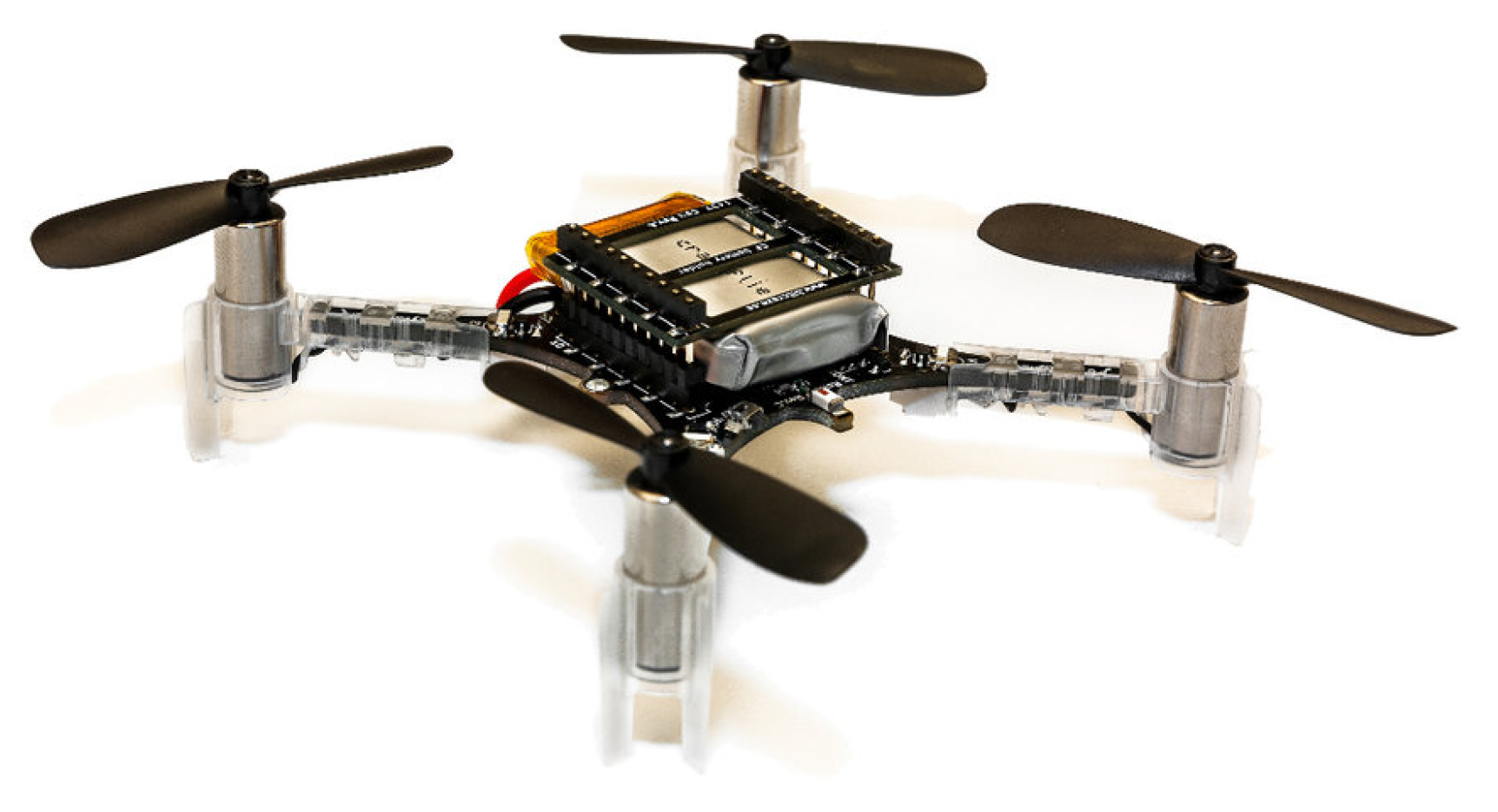
We chose a drone model for conducting our tests based on the open source development platform Bitcraze’s Crazyflie 2.0 [54]. Our model is a nanoquad, which is lightweight and small, allowing for better indoor flight and the ability to perform aggressive trajectories. The drone can be simulated in either a cross (reference body frame aligned with the drone arms) or equis (body axis at a 45-degree angle to the drone arms) configuration, and its features are listed in

Table 1. Bitcraze’s Crazyflie 2.0 Drone physical parameters.

Parameter	Description	Value
$m_{quad}$	Mass	270 [g]
Size	W × H × D	92 × 92 × 29 [mm]
d	Arm length	39.73 [mm]
r	Rotor ratio	23.13 [mm]
$I_{xx}$	Moment of inertia over x axis	1.395 × 10${}^{-5}$ [kg·m2]
$I_{yy}$	Moment of inertia over y axis	1.436 × 10${}^{-5}$ [kg·m2]
$I_{zz}$	Moment of inertia over z axis	2.173 × 10${}^{-5}$ [kg·m2]
$k_F$	Impulse coef.	3.160 × 10${}^{-10}$ [N/rpm2]
$k_M$	Torque coef.	7.940 × 10${}^{-12}$ [Nm/rpm2]
$C_{D_{xy}}$	Friction coef. over $xy$ axis	9.170 × 10${}^{-7}$
$C_{D_z}$	Friction coef. over z axis	10.31 × 10${}^{-7}$
$k_G$	Ground Effect coef.	$11.36$
$k_{D_1}$	Induced Flow coef. 1	2267
$k_{D_2}$	Induced Flow coef. 2	$0.160$
$k_{D_3}$	Induced Flow coef. 3	$-0.110$

and depicted in Figure 1.

As defined by Sabatino [13], the dynamics of the UAV in space, by assuming that ${\left[\begin{array}{ccc}\dot{\varphi }& \dot{\theta }& \dot{\psi }\end{array}\right]}^T={\left[\begin{array}{ccc}p& q& r\end{array}\right]}^T$, which is true for small angle motions, and ${\left[\begin{array}{ccc}\dot{x}& \dot{y}& \dot{z}\end{array}\right]}^T={\left[\begin{array}{ccc}u& v& w\end{array}\right]}^T$, would be defined by (1).

$$X=\left\{\begin{array}{cc}\ddot{x}=& -\frac{f_t}{m}\left[sin\left(\varphi \right)sin\left(\psi \right)+cos\left(\varphi \right)cos\left(\psi \right)sin\left(\theta \right)\right]\\ \ddot{y}=& -\frac{f_t}{m}\left[cos\left(\varphi \right)sin\left(\psi \right)sin\left(\theta \right)-sin\left(\varphi \right)cos\left(\psi \right)\right]\\ \ddot{z}=& g-\frac{f_t}{m}\left[cos\left(\varphi \right)cos\left(\theta \right)\right]\\ \ddot{\varphi }=& \frac{I_{yy}-I_{zz}}{I_{xx}}\dot{\theta }\dot{\psi }+\frac{{\tau }_x}{I_{xx}}\\ \ddot{\theta }=& \frac{I_{zz}-I_{xx}}{I_y}\dot{\varphi }\dot{\psi }+\frac{{\tau }_y}{I_{yy}}\\ \ddot{\psi }=& \frac{I_{xx}-I_{yy}}{I_{zz}}\dot{\varphi }\dot{\theta }+\frac{{\tau }_z}{I_{zz}}\end{array}\right.$$

(1)

Additionally, a vector of disturbances is defined in (2), mainly caused by changes in wind direction and magnitude, which alter the force and torque in each of the aircraft dimensions.

$$Z={\left[\begin{array}{cccccc}{f}_{wx}& f_{wy}& f_{wz}& {\tau }_{wx}& {\tau }_{wy}& {\tau }_{wz}\end{array}\right]}^T\in {\mathrm{I}\mathrm{R}}^6$$

(2)

3.1.2. DSLPID Controller

We have chosen Utia’s DSLPID controller as our baseline for training the Neural Networks. Our aim is to replicate the controller behavior using Deep Learning techniques. The DSLPID controller was developed initially by Jacopo Panerati et al. [55] at the University of Toronto Institute for Aerospace Studies (Utia) in their laboratory of dynamic systems (DSL).

Table 2. Parameters of the DSLPID controller.

Axis	${\mathit{k}}_{\mathit{P}}$	${\mathit{k}}_{\mathit{I}}$	${\mathit{k}}_{\mathit{D}}$
x	$0.40$	$0.05$	$0.20$
y	$0.40$	$0.05$	$0.20$
z	$1.25$	$0.05$	$0.50$
$\varphi$	70 × 10${}^3$	0.00	20 × 10${}^3$
$\theta$	70 × 10${}^3$	0.00	20 × 10${}^3$
$\psi$	60 × 10${}^3$	500	12 × 10${}^3$

shows the PID parameters obtained from the Mellinger controller [56] and designed for the model Bitcraze’s Crazyflie Cf2x/Cf2p [54]. The code for the Crazyflie controller is available on the GitHub of gym-pybullet-drones [57].

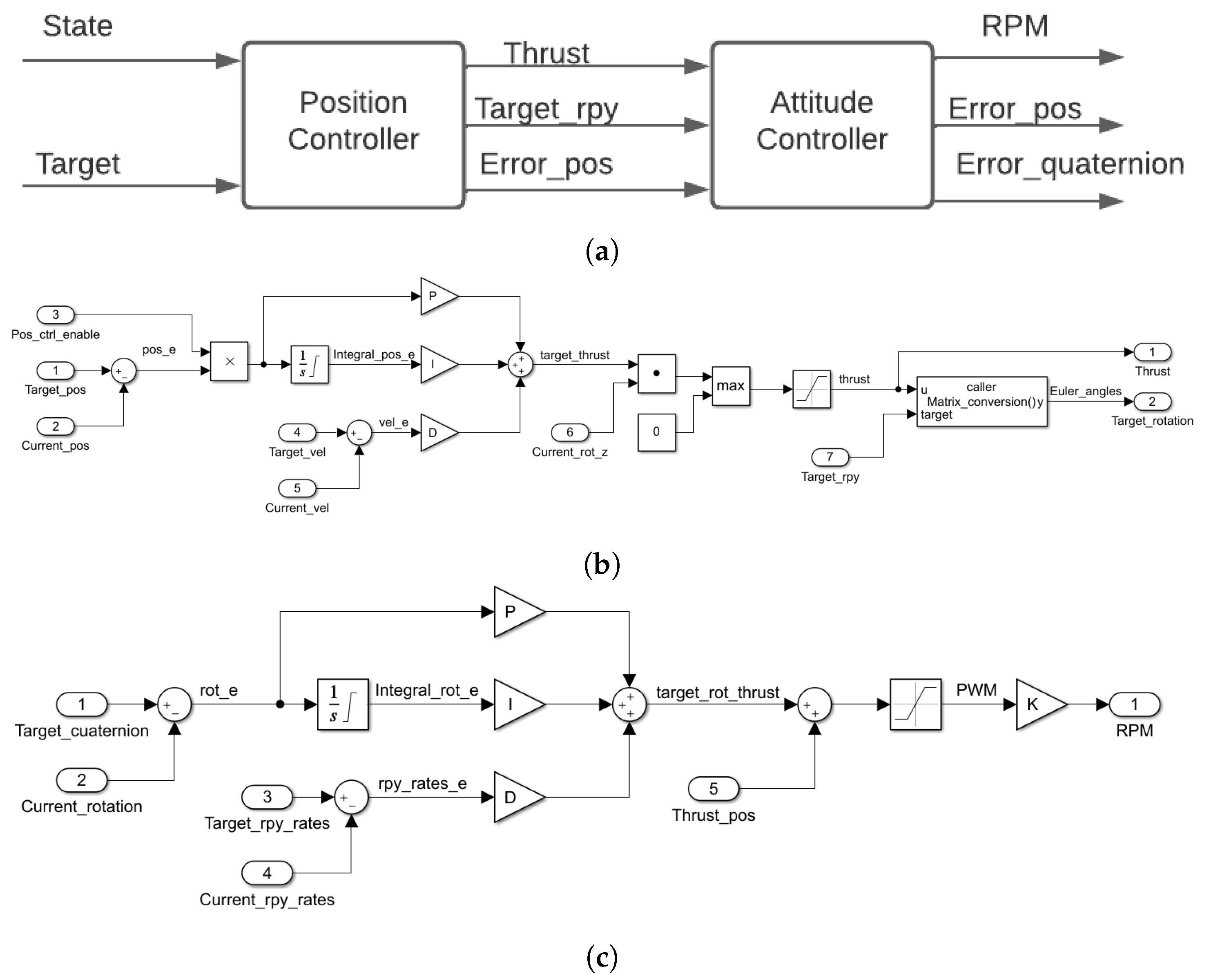
Figure 2a shows the general scheme of the controller. Due to a drone being an under-acted system, it is not possible to implement a straightforward controller for the x and y axis. It is necessary for a double loop controller to manipulate the mentioned axis by fixing the values of the $\varphi$ and $\theta$ axis. Then the controller will calculate a thrust value (which will act over the z-axis) to obtain a desired rotation that will move our drone in the $xy$ plane.

Inside, this controller is composed of PID controllers in the way that is displayed in Figure 2b,c for the position and attitude control, respectively.

3.1.3. Pybullet Set-Up

Along with the Pybullet framework, we use the gym-pybullet-drones project [58] and the OpenAI Gym library [59] to perform the Drone simulation.

• Open AI Gym: It is a tool kit developed to perform deep learning tasks. It allows one to design a simulation environment and works with several numeric calculation libraries such as TensorFlow [60].
• Gym-pybullet-drones: This open-source project is an environment from the Open AI Gym based on Pybullet, which has simulation tools for simulations with one and multiple agents. Furthermore, it allows the low-level control of aerial vehicles and emulation of aerodynamic effects such as friction, ground effect, and wind direction change.

To easily perform our simulations, we developed three classes: BaseControl, Drone, and PybulletSimDrone (you can find the developed software and a deeper explanation of these classes to implement it as well in our Git-Hub repository [61]).

• BaseControl defines the properties and methods of our drone controller according to its kind (for this project DSLPIDControl, SimplePIDControl, and NNControl). If we want to implement a PID controller (DSLPIDControl and SimplePIDControl), it will be necessary to define the $kp$, $kd$, and $ki$ coefficients for this controller. If we want to implement a Deep Neural Controller (NNControl), it will be necessary to define the file from Tensorflow (.h5) where our Neural Network is saved. This class contains methods to calculate the control signal and process the current states.
• Drone defines the drone properties, such as model, controller, initial position, and orientation. This class has methods to gather the current states from the environment and apply the control action.
• PybulletSimDrone defines the properties of our simulation environment required by Pybullet (such as physics engine, simulation frequency, control frequency, environment, and obstacles), debug options (such as graphic interface, video recording, console output, data graphics, and data storage); further, we define the trajectories to perform and whether we want to simulate with disturbances or not. The methods for this class allow one to initialize the environment, define drones and trajectories, debug the simulation, run one simulation step, and save state data).

Table 3. Parameters of the Pybullet environment.

Parameter	Value
Physics Engine	$Pyb$
Drone Model	$C2fx$
Controller	$DSLPID$
Simulation Frequency	240 Hz
Control Frequency	48 Hz
Obstacles	No
Environment	CtrlAviary

summarizes the environment parameters defined for this project.

3.2. Technical Specifications

The machine used for developing this investigation has an $AMD2950X\left(TM\right)$ $Threadripper\left(TM\right)$ $2950X$ processor, a NVIDIA GeForce RTX-2080Ti graphic card and 64 GB RAM. In terms of software to develop the experiments shown within this project. It is recommendable to use Python version 3.8.10, $gym\_pybullet\_drones$ 0.6.0, Pybullet 3.1.6 simulator, Gym 0.20.0, and the libraries for Python: $Numpy$ 1.19.5, $Matplotlib$ 3.3.4, $Statsmodels$ 0.12.2, Tensoflow-gpu 2.5.0, $Keras$ 2.5.0rc0, and $Keras\_tuner$ 1.0.3.

3.3. Dataset

In our proposed dataset, we want to collect data describing the behavior of our baseline controller in different states. To do so, we must first identify the information to be gathered from the environment. As a result, we read the input state vector (which was sent to the controller in Pybullet by the state estimator), which is shown in (3).

$$X={\left[\begin{array}{cccccccccccccccccc}\varphi & \hfill \theta & \psi & p& q& r& x& y& z& v_x& v_y& v_z& a_{\varphi }& a_{\theta }& a_{\psi }& a_x& a_y& a_z\end{array}\right]}^T\in {\mathrm{I}\mathrm{R}}^{18}$$

(3)

$$Y_{ref}={\left[\begin{array}{cccc}{r}_x& \hfill r_y& r_z& r_{\psi }\end{array}\right]}^T\in {\mathrm{I}\mathrm{R}}^4$$

(4)

$$u={\left[\begin{array}{cccc}RP{M}_0& \hfill RP{M}_1& RP{M}_2& RP{M}_3\end{array}\right]}^T\in {\mathrm{I}\mathrm{R}}^4$$

(5)

where u, v, and w are the linear speeds of the x, y, and z axes, respectively. p, q, and r are the angular speeds of the $\varphi$, $\theta$, and $\psi$ axes, respectively. Moreover, we derive the speed state vector provided by the estimator to get the acceleration vector. The derived variables are directly related to the input variables and may provide additional information that can potentially improve the accuracy of the model’s predictions. Reading in this way, all the variables of the current state. The reference position and orientation are depicted in (4). Finally, the Neural Network outputs are gathered in (5), and we read the four control signals for the actuator calculated by the reference controller.

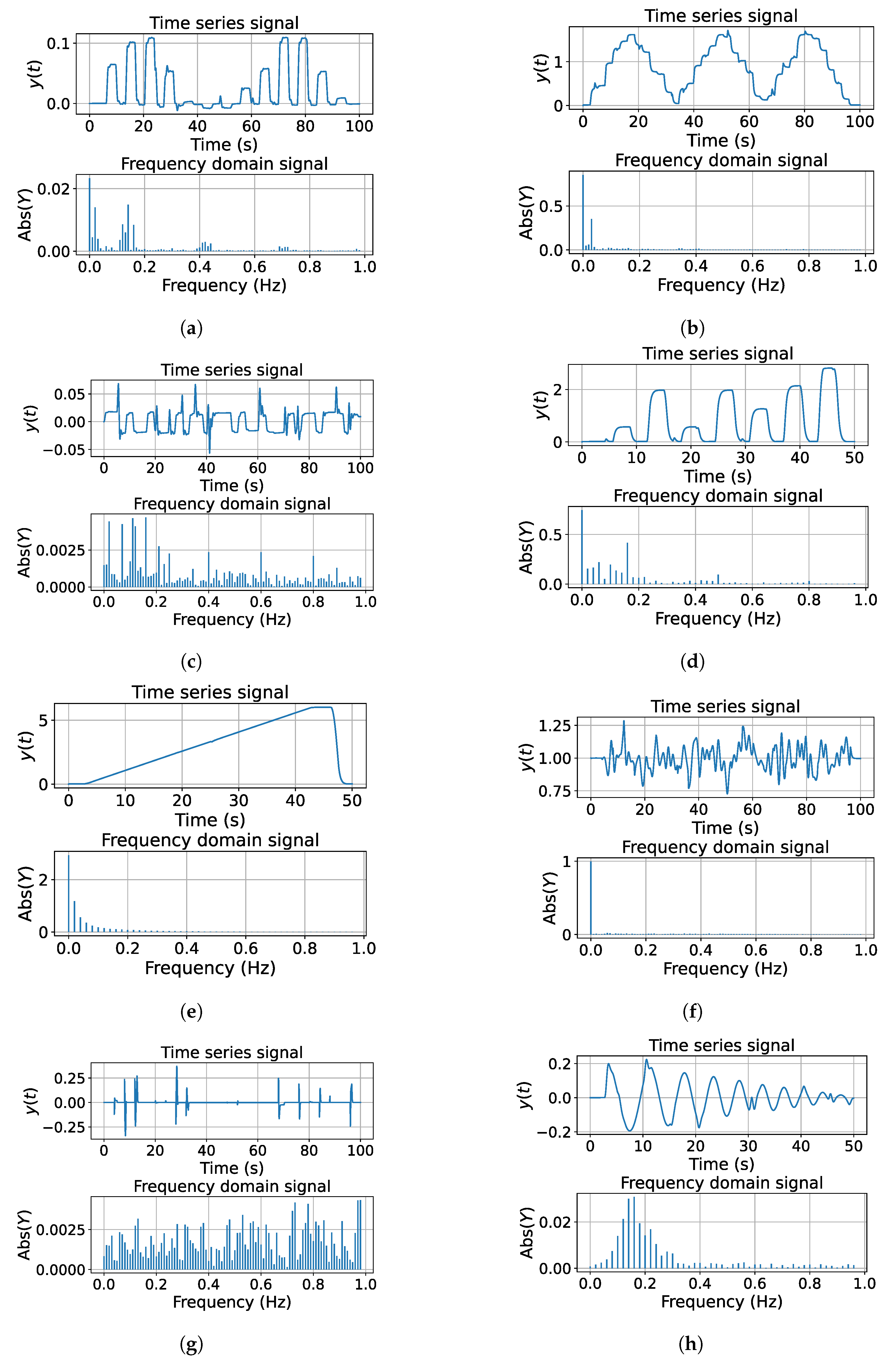
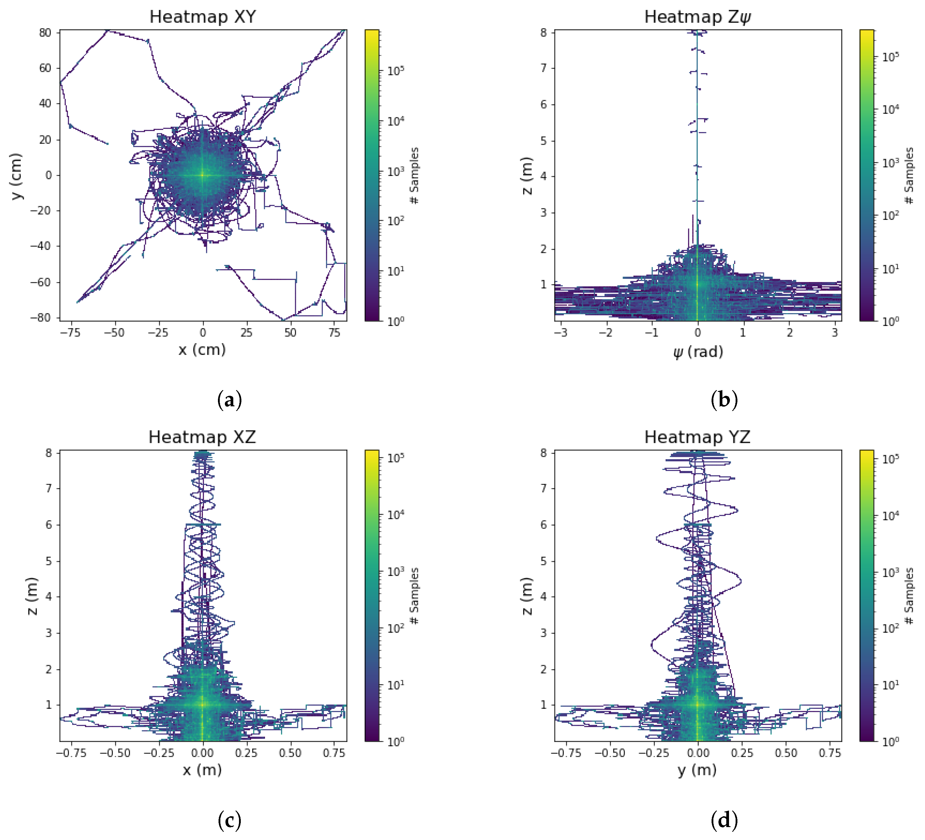
Once one defines all the variables to read from our environment, we proceeded to define the trajectories to save. We propose the trajectories presented in Figure 3.

The aim of these signals is to prioritize the number of harmonics, the normal distribution of data, and the balance between information at the transitory state and steady state. Moreover, some trajectories contain disturbances, where it will be possible to observe how the controller recovers in these scenarios. The process to generate this dataset is automatic; the trajectories for each axis and the parameters of these were chosen randomly. We dismissed the signals when the drone fell or was not possible to track the trajectory.

3.4. Time Window

Due to the signals of the system being a time series, it is important to feed previous states to our Neural Networks so that it is possible for the network to calculate the control signal for each motor. We will define a number of previous states where we find a balance between inference time, memory size, and performance of our models.

3.4.1. Partial Autocorrelation Function

This function is defined in (6).

$${\rho }_k=\frac{{\sum }_{t=1}^{N-K}(x_t-\mu )(x_{t+k}-\mu )}{{\sum }_{t=1}^N{(x_t-\mu )}^2}$$

(6)

where x is our signal, composed of the current state and the previous states, and $\mu$ is the average of our data, defined as $\mu ={\sum }_{t=1}^N\frac{x_t}{N}$.

This function calculates the autocorrelation between the current state and the previous states. A positive correlation value means a strong association between the values of the current state and previous states [62].

For our case, we calculate the autocorrelation taking signals from our dataset for each axis. Getting the autocorrelation value for several quantities of states in a range of 1 to 100.

Table 4. The quantity of samples with the highest autocorrelation.

Position	x States	y States	z States	$\mathit{\psi }$ States	Median
1	75	2	76	57	2
2	60	63	59	66	75
3	93	5	2	4	58
4	29	96	40	78	64
5	2	21	47	40	67

shows in descending order the quantity of states per axis where we found the highest autocorrelation.

Taking the median per axis, we find that the highest autocorrelation value is obtained with the two previous states. However, taking into account the simulation frequency and the rise times per axis of our baseline controller, this is a small amount of information for our Neural Network. Hence we take a number of the previous states between the third and second highest value of autocorrelation (58 and 75).

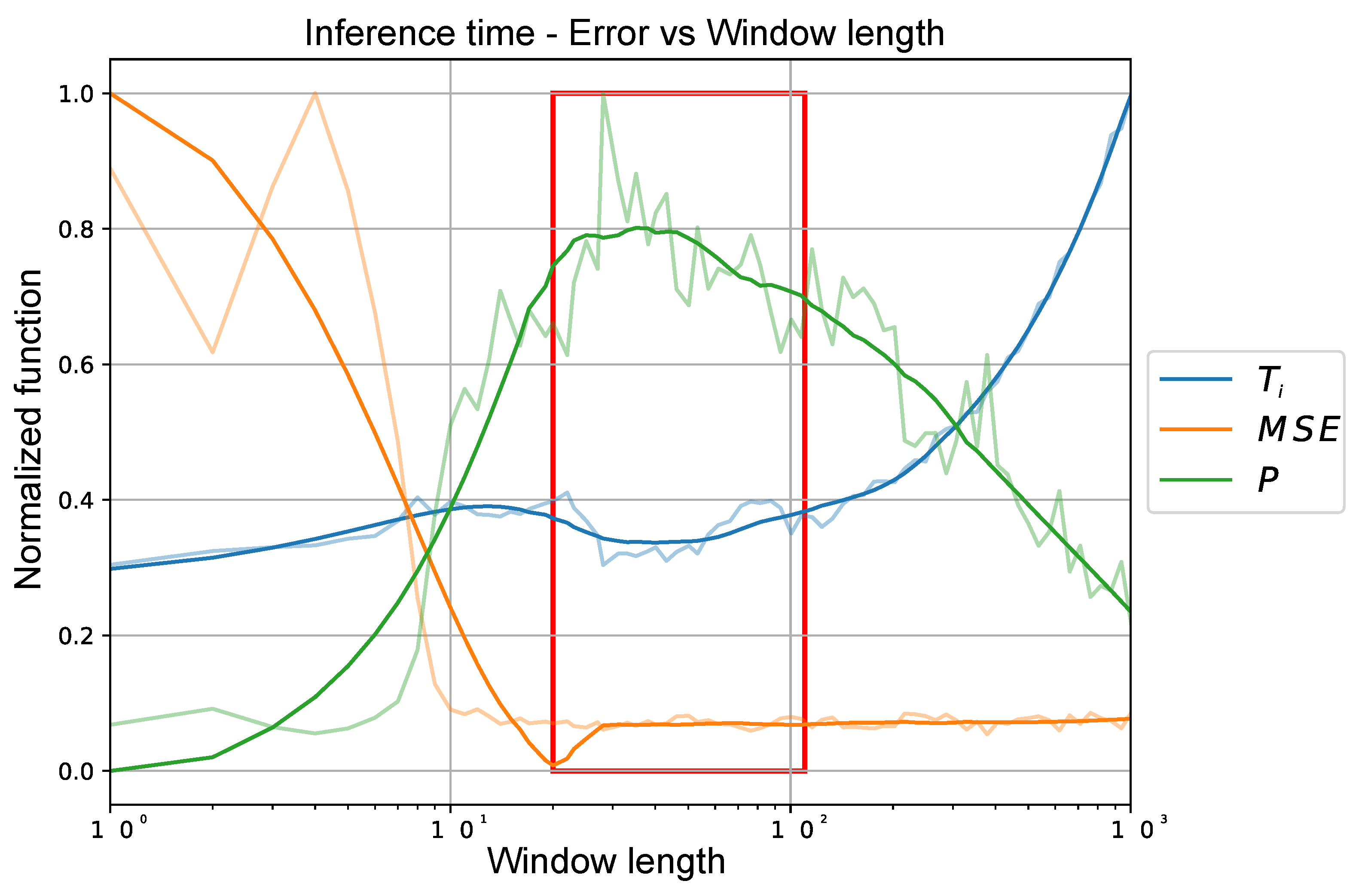
3.4.2. Empirical Method

This method relies on taking into account the Average Inference Time ($T_i$) and Mean Square Error ($MSE$). We sweep the Time Window sizes between a range of 1 to 1000, taking 100 window sizes that are separated logarithmically along the defined range. To evaluate the performance of our model, we use a dataset size of 4096 samples obtained from our dataset and measure $MSE$ as well as $T_i$ for the samples passed to our model. Finally, we calculate the performance (P) with the function defined in (7).

$$P=\frac{1}{MSE\times T_i}$$

(7)

Figure 4 shows the values of this function for the described range, where the optimal value is between the values of 20 to 90 previous states as shown in Figure 4 by the red square.

Due to both tests of the previous states, it is defined as a quantity in the middle of the found ranges. Hence the size of our time window will be 63 previous states plus the current state because it is a multiplot of 2 and could be advantageous in the implementation.

3.5. Data Pre-Processing

First, we apply average normalization to the data. We normalize each signal presented in the state vector (Section 3.3) according to the function presented in (8).

$$x_{nor{m}_i}=\frac{x_i-\mu }{x_{max}-x_{min}}$$

(8)

where $\mu$ is the average value of the signal; $x_{max}$ and $x_{min}$ are maximum and minimum values, respectively; and $x_i$ is the signal’s sample to normalize.

Later, we sort our data into three batches (train, validation, and test), of which the portions are shown in

Table 5. Dataset division.

Batch	Quantity of Trajectories	Percentage
Train	142	$84\%$
Validation	16	$10\%$
Test	10	$6\%$

.

Finally, we define a Data Generator Class from Tensorflow per batch [63]. This helps us to select the data while training. To create one sample, our generator takes a current random state from our normalized dataset and appends it to the previous states; subsequently, the data are sorted according to the input sizes required for each net architecture. In this way, the generator creates samples until it fulfills the defined batch size. Once this process is done, the batch is provided to perform one episode of our Neural Network training. The previous process is performed iteratively by the generator until it finishes the training.

3.6. Proposed Architectures

To model the behavior of the controller, we propose analyzing several types of Neural Network architectures:

(i)

Fully Connected Artificial Neural Networks (ANN): These networks are also known as Multi-Layer Perceptrons (MLPs) or Feedforward Neural Networks (FNN). This architecture is the simplest and also the architecture that consumes the least resources. They consist of multiple layers of nodes (neurons) connected in a feedforward manner, where each neuron in a layer is connected to all the neurons in the previous layer. ANNs are suitable for modeling nonlinear relationships between inputs and outputs, which makes them suitable for modeling the behavior of a position PID controller.

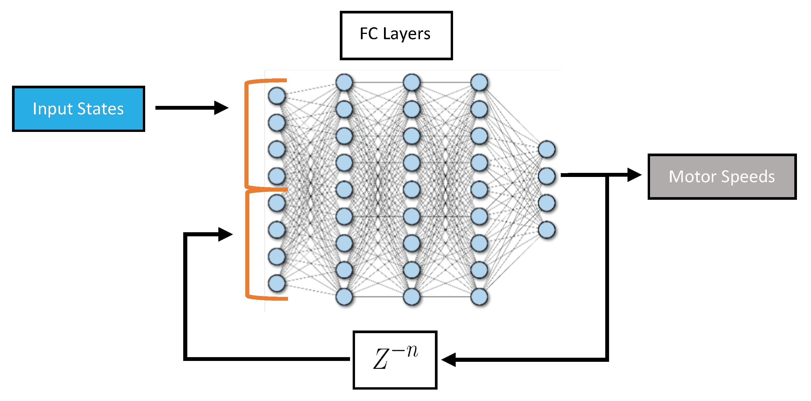
(ii)

Fully Connected Artificial Neural Networks with Feedback (ANN Feedback): This architecture is sometimes referred to as an autoregressive model or iterative prediction. It is based on ANN, but the input states include the previous output of the network as illustrated in Figure 5. It can allow the network to incorporate information about past predictions into future predictions. This could be particularly useful in applications where the system being controlled is dynamic and subject to rapid changes.

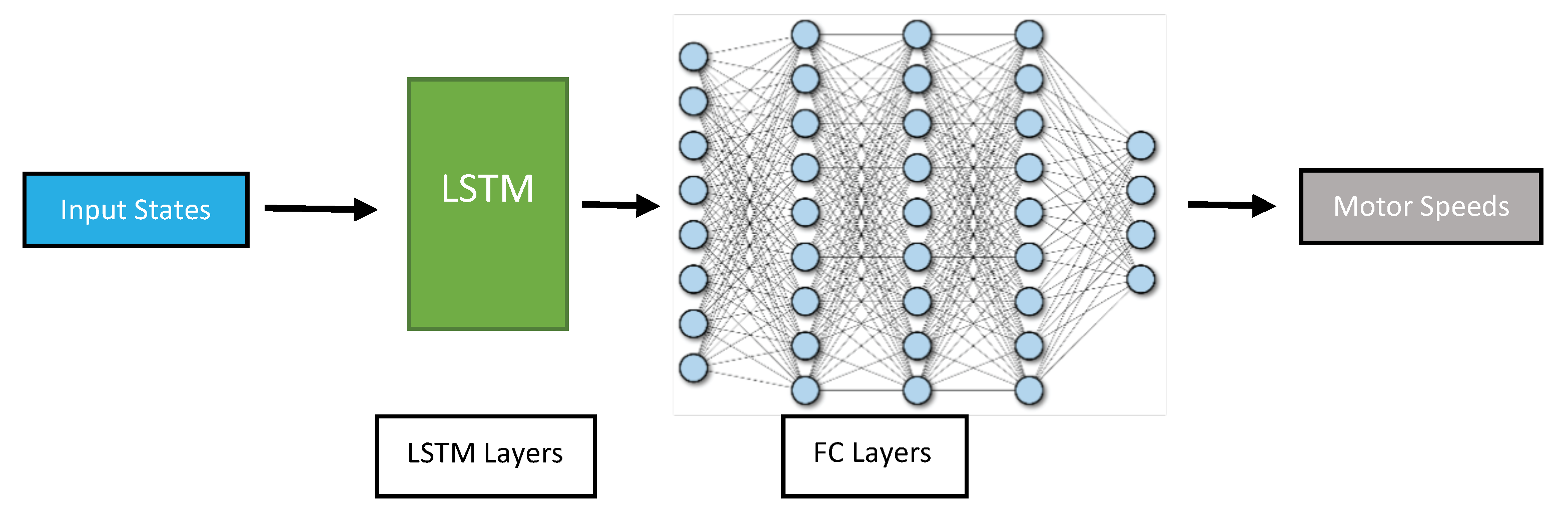
(iii)

Long-Short Term Memory (LSTM): These networks are a type of Recurrent Neural Network (RNN) that are designed to handle long-term dependencies in sequential data such as time series data. They use a memory cell to store information over time, which allows them to maintain a long-term memory of past observations. It can be used to learn the patterns and dynamics of the drone’s movements over time. One potential advantage of using an LSTM for drone position control is its ability to handle variable-length input sequences. This can be particularly useful in situations where the drone’s movements are not perfectly regular or predictable: the input sequence could be longer or shorter depending on the complexity of the environment and the level of variability in the conditions. The proposed architecture is shown in Figure 6.

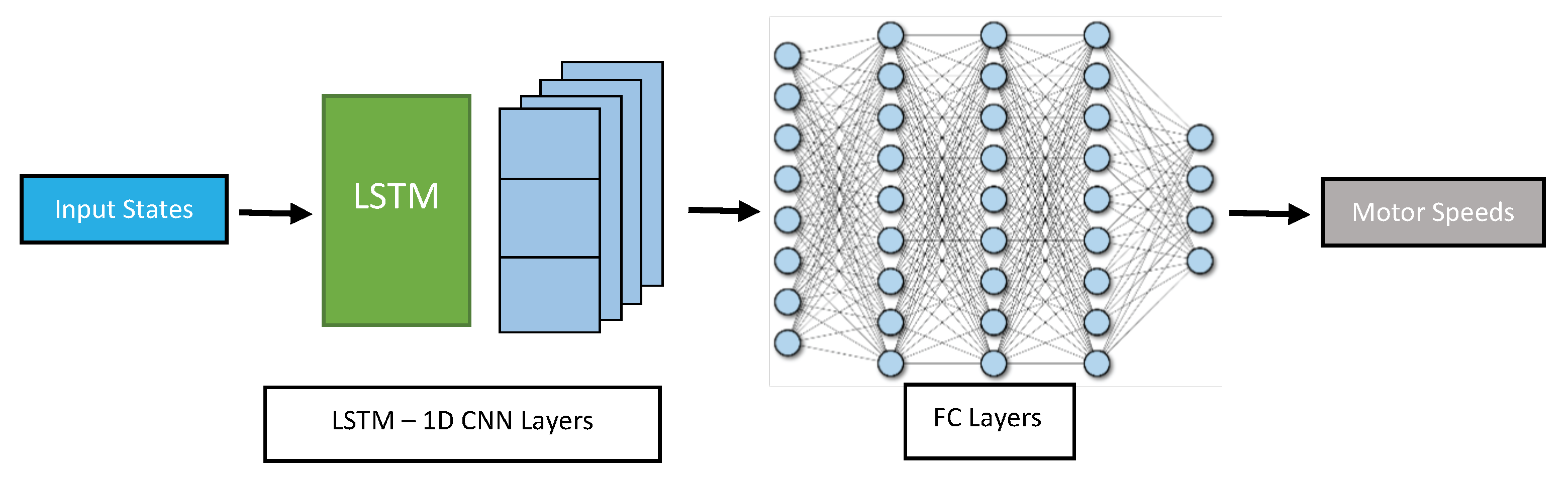
(iv)

LSTM Layers interleaved with convolutional 1D layers (LSTMCNN): This architecture consists of connected blocks in a cascade at the beginning of the network, where each block is composed of LSTM layers followed by convolution layers in one dimension (CNN-1D) as shown in Figure 7. The CNN-1D can capture local patterns and features in the sequential data, while the LSTM can capture long-term dependencies and context. The output of each block can be fed into the next block, allowing for a hierarchical feature extraction process in both time and frequency domains. The fully connected layers can further process the extracted features and generate the final output. Both CNN-1D and LSTM can handle variable length sequences of data. CNN-1D is also robust to noise and variability in the input data.

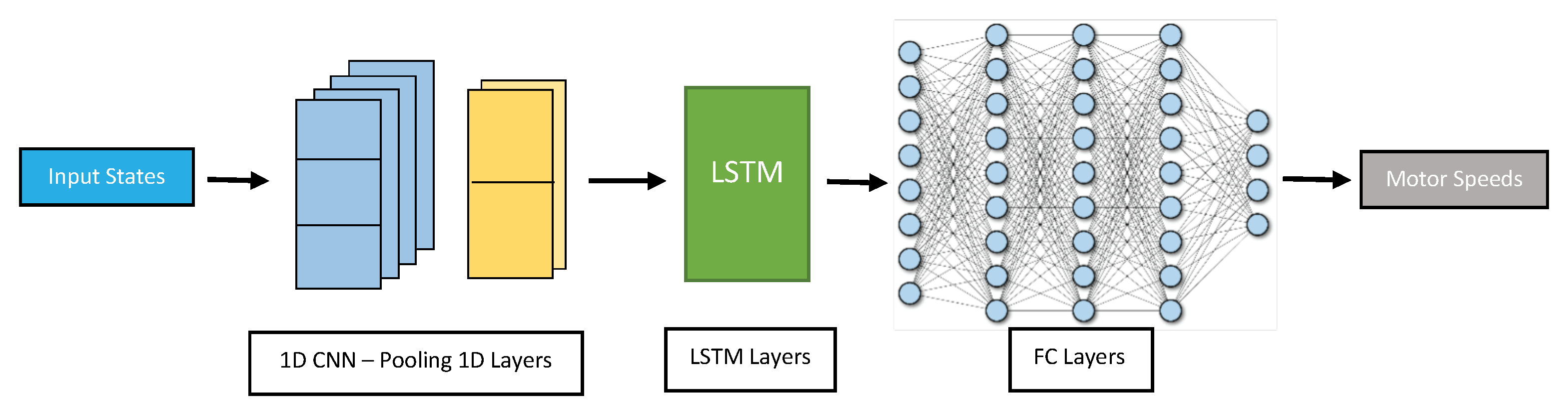
(v)

Convolutional 1D Layers in cascade with LSTM layers (CLSTM): This proposed architecture consists of connected blocks in a cascade at the beginning of the network, where each block is composed of convolutional 1D layers followed by max pooling layers to identify the most salient features in the data by taking the maximum value within a pooling window. The output of each block can be fed into LSTM layers, which can capture the long-term dependencies in the drone’s flight path based on the most important features extracted from the convolutional layers. The output of the LSTM layers can then be fed into several fully connected layers in a cascade to process the extracted features further and generate the final output as shown in Figure 8.

Model Compilation and Hyper-Parameter Tuning

For this stage, the Neural Network model is defined according to the desired architecture to train. It is defined as an optimizer, a loss function, activation functions, a gradient clipping value to avoid gradient exploding (specifically for the most complex architectures, which include LSTM and Convolutional layers), and some other hyper-parameters. These values were obtained from the evaluation of the final error in numerous randomly combined hyper-parameter training carried out experimentally. The values of the previously mentioned Hyper-parameters are summarized in

Table 6. Hyper-parameter definitions.

Parameter	Value
Loss function	MSE
Optimizer	Adam
Gradient clipping	0.5
Batch size	1024
Time window size	64
Hyperband max epochs	500
Hyperband executions per trial	2
Hyperband reduction factor	3
Training steps	142
Validation steps	16
Pooling type	max
Pooling kernel size	3
LSTM activation	tanh
LSTM recurrent activation	Sigmoid

.

For each of the architectures, hyper-parameters such as the number of neurons per layer, the number of layers, and the activation function of each neuron were obtained using the Hyperband algorithm [51], as shown in

Table 7. Hyper-parameter tuning objectives.

Parameter	Default	Min	Max	Step	Values
LSTM Layers	5	1	5	1
LSTM Units	256	32	512	32
CNN-1D Layers	5	1	5	1
CNN-1D filters	128	32	512	32
CNN-1D Activation	relu				[relu, tanh, sigmoid]
FC Layers	5	1	5	1
FC Units	128	32	512	32
FC activation	relu				[relu, tanh, sigmoid]
Learning rate	1 × ${10}^{-3}$	1 × ${10}^{-4}$	1 × ${10}^{-2}$	log

. Hyperband is designed to efficiently allocate resources, such as computation time or hardware resources, to explore the hyper-parameter space and find the best set of hyper-parameters for a given machine learning model.

Once these values are defined, the training starts. Subsequently, we briefly evaluate the trained model according to its mean square error value with the test data batch.

3.7. Evaluation Functions

The evaluation of the proposed system focuses on reducing energy consumption and error in trajectory tracking, as shown below.

3.7.1. Control Effort

To evaluate the control effort for our controllers, we apply (9) by comparing the output signal $u\left(t\right)$ with $u_{ss}$, which is the magnitude from the controller output to counteract gravity (this value is 14,468.429).

$$Q=\frac{1}{t}{\int }_0^T|u\left(t\right)-u_{ss}|\delta t$$

(9)

where T is the integration time from the total duration of the simulation.

3.7.2. F1 Custom Function

This function rates the performance in terms of Settling Time (Ts), Overshoot (Os), and Steady State Error (sse) with the ITSE function as indicated in (10)–(13).

$$Ts\to \left|y\left(t\right)-y_{final}\right|<0.02\times y_{final}$$

(10)

$$Os=\frac{max\left(y\left(t\right)\right)-y_{final}}{y_{final}}$$

(11)

$$ITSE=\frac{1}{len\left(t\right)}\sum _{i=1}^{len\left(y\right(t\left)\right)}t\ast {\left(y_i-u\right)}^2$$

(12)

$$F1=\frac{(a\ast Ts)+(b\ast Os)+(c\ast ITSE)}{3}$$

(13)

where $y\left(t\right)$ is the series of position values in the evaluated axis and $y_{final}$ is the final value in the evaluated axis. Moreover, a, b, and c are the weights of function F1 whose aim is to compare each value in each function for the proposed controllers compared with our reference PID. Those weights are defined as the multiplicative inverse of the scores assigned by each function to our PID baseline as depicted by (14).

$$a=\frac{1}{T{s}_{PID}};b=\frac{1}{O{s}_{PID}};c=\frac{1}{ITS{E}_{PID}}$$

(14)

4. Results

The results obtained from the experimentation of the proposed model are shown based on the performance of the different models proposed in terms of stability, energy consumption, and path tracking.

4.1. Final Dataset

The final dataset and specific features are explained next. This dataset is fundamental in the training process of the different models used.

4.1.1. Main Features

Our final dataset applied to train each model is composed of 168 trajectories with a duration between 15 and 100 s. Those trajectories are distributed as described in

Table 8. Dataset description.

Parameter	Value
Length	168 signals
Size	0.778 GB
States	18 variables
Set-Point	4 variables
Outputs	4 variables
Average simulation time	76.55 s
Total samples	3.068 × 10${}^6$

,

Table 9. Trajectories per duration.

Duration	Quantity
100 s	104
50 s	38
20 s	22
15 s	4

and

Table 10. Number of trajectories per type of trajectory and axis.

Type of Trajectory	X	Y	Z	$\mathit{\psi }$	Total
Null reference with disturbances	46	56	44	99	245
Random step with return to zero	61	63	66	53	243
Staggered random steps	23	17	20	3	63
Low frequency noise	7	8	19	4	38
Sinusoidal wave	15	6	11	4	36
Staggered sinusoidal with return to zero	9	10	3	1	23
Chirp Signal	2	2	0	0	4
Others 1	5	6	5	4	20

¹ Composed by test signals (ramps, lemniscate, and exponential).

.

4.1.2. Data Distribution

Table 11. Descriptive statistics for control variables.

Axis	Mean	Std	Min	Max
$r_x$	6.439 × 10${}^{-3}$	1.058 × 10${}^{-1}$	−8.000 × 10${}^{-1}$	8.000 × 10${}^{-1}$
$r_y$	3.417 × 10${}^{-3}$	1.010 × 10${}^{-1}$	−8.000 × 10${}^{-1}$	8.000 × 10${}^{-1}$
$r_z$	8.782 × 10${}^{-1}$	7.641 × 10${}^{-1}$	$0.000$	$7.998$
$r_{\psi }$	1.285 × 10${}^{-2}$	4.414 × 10${}^{-1}$	−3.140	$3.141$

provides descriptive statistics for the control variables in the dataset. These statistics offer insights into the rank, dispersion, and distribution characteristics.

To determine the maximum and minimum values for the trajectories, we identified the empirical values at which the controller remained stable. Additionally, we estimated the average value to approximate the operating point $X_0={\left[\begin{array}{cccc}\overline{x}=0& \overline{y}=0& \overline{z}=1& \overline{\psi }=0\end{array}\right]}^T$ around which the controller was designed.

The data distribution for variables x, y, and $\psi$ follows a Gaussian distribution, while the distribution for variable z is asymmetrical and primarily concentrated at lower altitudes. These characteristics provide important insights into the behavior and range of the control variables in the dataset.

To evaluate the range of position exploration in our dataset and identify states with less information during model training, we created Figure 9. This visualization provides insights into the generalization of the model’s behavior and highlights areas where the dataset may have limited coverage.

4.2. Neural Network Architectures

This section explains the process of obtaining the best neural controller from all the proposed architectures. In this selection process, first, for each proposed architecture, we manually and automatically tuned our models until getting the best five models taking into account the MSE loss function. The models tuned automatically were the models that involved CNN1D and LSTM layers within its architecture, due to the complexity of these models. The algorithm used to tune our models automatically was the Hyperband algorithm [51]. Figure 10 shows the loss per epoch for the trained models. A total of 64 models per architecture type were trained using the Hyperband algorithm. These five architectures were tested in simulation to choose the best model per architecture. The simulation was performed under one specific scenario, where our drone had to follow a step set-point signal in each axis ($r_x=0.1$ m, $r_y=0.1$ m, $r_z=0.1$ m, $r_{\psi }=0.1$ rad). To evaluate the performance of each controller in the simulation, we implemented the personalized function F1.

Table 12. Best models comparison.

Architecture	MSE	$\mathit{F}{1}_{\mathit{x}}$	$\mathit{F}{1}_{\mathit{y}}$	$\mathit{F}{1}_{\mathit{z}}$	$\mathit{F}{1}_{\mathit{\psi }}$	$\mathit{F}{1}_{\mathbf{avg}}$	Q	Total
ANN	3.31 × ${10}^{-3}$	0.31	0.70	6.48	28.3	8.95	415 × ${10}^3$	7.44
LSTM	2.36 × ${10}^{-3}$	0.98	1.10	27.8	18.2	12.0	69.7 × ${10}^3$	6.51
LSTMCNN	3.27 × ${10}^{-3}$	1.39	0.97	10.6	23.7	9.17	59.3 × ${10}^3$	5.01
CLSTM	2.39 × ${10}^{-3}$	1.44	1.07	27.7	19.0	12.32	79.3 × ${10}^3$	6.73
DSLPID	NA	1	1	1	1	1	70.0 × ${10}^3$	1

relates the evaluation parameters for each of the best-obtained models per architecture. Figure 11 shows the step time response for the best model for each of the proposed architectures.

Table 12 provides the evaluation metrics for the different models considered in our study. The mean square error (MSE) quantifies the average squared difference between the predicted and target values. The control effort (Q) is measured using (9), and $F{1}_{avg}$ represents the average total score per axis based on time response parameters.

To assess the overall performance of each model, we introduce the “Total” value, which incorporates the normalized values of Q and $F{1}_{avg}$ (denoted as $Q_{norm}$ and $F{1}_{norm}$, respectively). The calculation of the Total value is explained in (15)–(17). We would like to note that the ANN Feedback architecture is not included in our study due to its inherent instability in simulation. Therefore, we focused our analysis on the other architectures to select the most suitable model for our purposes, with LSTMCNN emerging as the optimal choice based on its performance in terms of control effort and F1 error. The specific structure of the LSTMCNN model is presented in

Table 13. LSTMCNN 5 Structure.

Layers	Neurons/Filters	Activation	# Parameters
LSTM_1	320	tanh	439 K
CONV1D_1	480	relu	461 K
LSTM_2	128	tanh	311 K
CONV1D_2	288	relu	110 K
LSTM_3	128	tanh	213 K
FC_1	64	relu	8 K
FC_2	96	relu	6 K
FC_3	320	relu	31 K
FC_4	192	relu	61 K
FC_5	4	linear	772

.

$$Q_{norm}=\frac{Q}{70.01 \times {10}^3}$$

(15)

$$F{1}_{norm}=\frac{F{1}_{avrg}}{1}$$

(16)

$$Total=\frac{Q_{norm}+F{1}_{norm}}{2}$$

(17)

4.3. LSTMCNN Comparison with PID Baseline

In this section, we present a comprehensive evaluation and comparison of our proposed Neural Network Controller, the LSTMCNN, with the baseline controller, DSLPID controller, for UAV position control. Our objective is to assess the performance and effectiveness of the Neural Network Controller in various aspects and compare it to the baseline controller to gain insights into its advantages and limitations. The evaluation encompasses multiple criteria, including the response in the time domain (Section 4.3.1), control limits (Section 4.3.2) disturbance rejection (Section 4.3.3), sensitivity to noise (Section 4.3.4), handling aggressive trajectories (Section 4.3.5), adaptability (Section 4.3.6), and stability analysis (Section 4.3.7).

4.3.1. Step Response

For this test, we compare the basic control evaluation parameters towards a step set-point signal in each control axis ($r_x=0.2$ m, $r_y=0.2$ m, $r_z=0.2$ m, and $r_{\psi }=0.2$ rad), the results are shown with the Figure 12 and Figure 13.

Table 14. Step response measures.

Axis	DSLPID				LSTMCNN
	Ts [s]	Os [%]	Ess [ITSE]	F1	Ts [s]	Os [%]	Ess [ITSE]	F1
x	5.12	5.786	1725	1.000	1.750	8.687	4326	0.983
y	5.15	5.813	1737	1.000	2.680	7.322	2412	0.970
z	0.816	0.134	88.38	1.000	1.470	2.388	1097	10.64
$\psi$	0.808	2.247	225.2	1.000	3.170	0.269	15,109	23.70

shows the measures of this experiment.

4.3.2. Big Step Response

In our experiment, we aimed to compare the behaviors of the DSLPID controller and our LSTMCNN controller under a larger magnitude step input, which can lead to output saturation and consequently trigger the wind-up effect. The wind-up effect is a phenomenon observed especially with PID controllers, where the integral term accumulates excessive error, resulting in undesired outcomes such as overshoot, instability, or slow response. In the context of UAV position control, the wind-up effect can manifest when the drone encounters external disturbances or movement limitations, such as reaching maximum velocity or encountering physical obstacles. The time domain responses of both controllers to the larger step input can be observed in Figure 14.

Our objective was to assess how the controllers perform under these challenging conditions and observe if the Neural Network Controller exhibits a broader range of responses beyond the nominal operating point. As anticipated, the DSLPID controller demonstrated the wind-up effect in our experiment, resulting in instability. On the other hand, our Neural Network Controller, the LSTMCNN, showcased a wider range of responses that surpassed the nominal operating point. However, it is worth noting that the response in the $\psi$ axis exhibited instability, and there is room for improvement in the z axis. This behavior indicates the potential of the LSTMCNN controller to handle larger step inputs and adapt to varying conditions, offering improved performance compared to the PID controller.

4.3.3. Disturbance Rejection

For this experiment, we compare the disturbance rejection with disturbances twice as large compared to those present in the dataset, the results are presented in Figure 15.

Table 15. Disturbance response measures.

Axis	DSLPID				LSTMCNN
	Ts [s]	Os [%]	Ess [ITSE]	F1	Ts [s]	Os [%]	Ess [ITSE]	F1
x	4.904	2.946	72.89	1.000	5.216	2.765	301.2	26.74
y	4.904	2.853	70.24	1.000	7.045	1.988	50.17	1.594
z	1.058	8.672	145.1	1.000	2.062	9.615	1725	12.83
$\psi$	2.783	10.09	71.28	1.000	3.712	11.99	1224	19.07

shows the measures of this experiment.

4.3.4. Noise Degradation

Noise in the input can originate from various sources, including sensor inaccuracies, measurement errors, and environmental disturbances affecting the drone. By quantifying the impact of noise on the controller’s performance and providing a comparison to the ideal conditions, we can gain insights into the model’s robustness and assess its ability to handle noisy input conditions. Therefore, the objective of this experiment is to assess the model’s response to noisy conditions and analyze its effect on the controller’s performance.

To introduce noise, we determined the noise variance based on the rank of each variable and used (18) to establish the relationship. The noise variance values are provided in

Table 16. Noise parameters.

Axis	Variance
x	8.180 × 10${}^{-3}$ [m]
$v_x$	1.002 × 10${}^{-2}$ [m/s]
$a_x$	4.093 × 10${}^{-1}$ [m/s2]
y	8.176 × 10${}^{-3}$ [m]
$v_y$	8.609 × 10${}^{-3}$ [m/s]
$a_y$	3.494 × 10${}^{-1}$ [m/s2
z	4.037 × 10${}^{-2}$ [m]
$v_z$	6.607 × 10${}^{-2}$ [m/s]
$a_z$	$1.009$ [m/s2]
$\psi$	3.141 × 10${}^{-3}$ [rad]
r	7.241 × 10${}^{-2}$ [rad/s]
$a_{\psi }$	$2.080$ [rad/s2]

, and a uniform distribution was chosen for all axes.

$$\Delta =1\%\ast \frac{(X_{max}-X_{min})}{2}$$

(18)

where $X_{max}$ and $X_{min}$ are the maximum and minimum values of the state variable, respectively.

Subsequently, we simulated the controller using a zero reference signal and added noise to the model input for each state variable individually, corresponding to its respective control axis. For example, when analyzing the response in the z-axis, we introduced noise in variables z, $v_z$, and $a_z$. The time responses for x, y, z, and $\psi$ are illustrated in Figure 16, Figure 17, Figure 18 and Figure 19, respectively.

The degradation in controller performance caused by noise is presented in

Table 17. Noise signal degradation measurements.

Axis	DSLPID			LSTMCNN
	Pos.%	Vel. %	Acc. %	Pos. %	Vel. %	Acc. %
x	$0.562$	5.684 × 10${}^{-3}$	$0.000$	$0.597$	4.807 × 10${}^{-3}$	24.15 × ${10}^{-3}$
y	$0.560$	4.190 × 10${}^{-3}$	$0.000$	$0.559$	4.029 × 10${}^{-3}$	9.418 × 10${}^{-3}$
z	$13.57$	$0.131$	$0.000$	$20.21$	$12.33$	$10.43$
$\psi$	$8.923$	$0.000$	$0.000$	$9.492$	82.02 × 10${}^{-3}$	$2.614$

. This degradation is calculated as the difference between the ideal operation without noise and the performance under noisy conditions, as shown in (19). It is important to note that the baseline controller does not utilize acceleration information for the control action calculation, and for the R-axis, speed information is also excluded.

$$SigDegradation\%=\frac{MSE(x_{noise},x)}{\Delta }\ast 100\%$$

(19)

4.3.5. Lemniscate

In this experiment, our objective was to evaluate the performance of the controllers when subjected to aggressive set points. We specifically chose a Lemniscate function as the set-point signal, which follows an infinite (∞) shape. The use of this function is motivated by the need for high speeds and large attitude angles, which take the drone away from its linear operating point, posing a challenge for linear controllers such as the PID controller to track the signal accurately. The Lemniscate function is implemented as shown in (20).

$$\begin{array}{c}\hfill x\left(t\right)=\left(a\sqrt{2}\right)\frac{cos(2\pi f\ast t+\Psi )}{si{n}^2(2\pi f\ast t+\Psi )+1}\\ \hfill y\left(t\right)=x\left(t\right)sin(2\pi f\ast t+\Psi )\end{array}$$

(20)

where a is the amplitude, f the frequency, and $\Psi$ the offset angle.

The responses of both controllers to the Lemniscate set-point signal are depicted in Figure 20. It is evident from the results that the LSTMCNN neural network controller successfully tracks the intricate shape of the Lemniscate function, demonstrating its capability to handle the demanding trajectory. In contrast, the baseline PID controller struggles to follow the desired trajectory, which eventually leads to instability accurately. These findings highlight the superior performance and robustness of the LSTMCNN controller in challenging scenarios with aggressive set points.

4.3.6. Down-Wash Effect

In this experiment, our objective is to evaluate whether our controllers, the DSLPID (PID controller) and the LSTMCNN (Neural Network), demonstrate generalization capabilities for aerodynamic effects that were not considered in our dataset due to limitations in the physics engine used. Specifically, we focus on investigating the downwash effect by incorporating it into our simulation. The downwash effect is the change in airflow caused by the aerodynamic interaction of an aircraft. When two quadcopters cross paths at different altitudes, the lower drone experiences a reduction in lift force. Panerati et al. [55] modeled this effect by applying a force to a point particle, where the magnitude W depends on the distances in the x, y, and z axes between the two vehicles (${\delta }_x$, ${\delta }_y$, ${\delta }_z$), as well as experimentally derived constants $k_{D_1}$, $k_{D_2}$, $k_{D_3}$:

$$W=k_{D_1}{\left(\frac{r_P}{4{\delta }_z}\right)}^{2}exp\left(-\frac{1}{2}{\left(\frac{\sqrt{{\delta }_x^2+{\delta }_y^2}}{k_{D_2}{\delta }_z+k_{D_3}}\right)}^2\right)$$

(21)

The constants $k_{D_1}$, $k_{D_2}$, and $k_{D_3}$ capture the characteristics of the aerodynamic interaction, allowing for accurate modeling of the force experienced by the lower drone. To achieve this, we select the $pyb\_dw$ physics engine in our simulator and conduct the simulation with two drones, each equipped with one of our controllers (DSLPID and LSTMCNN).

To compare the performance of the controllers under the downwash effect, the drones fly in close proximity, with one drone positioned below the other to experience the downwash effect in its flight. Both drones follow sinusoidal trajectories that are out of phase with each other. The response of both controllers is illustrated in Figure 21.

4.3.7. Phase Plane Evaluation

In this experiment, our focus is to assess the robustness of our LSTMCNN controller and compare it with the baseline DSLPID controller using a phase-plane evaluation. The phase plane offers a visual representation that enables us to comprehend the system’s behavior in relation to its state variables. This analysis provides valuable insights into the controllers’ responses to various set-point signals and disturbances.

To achieve our objective, we examine the responses of both controllers in terms of position and speed for each axis within the phase plane. Specifically, we evaluate their performance under different set-point signals, including sinusoidal, step, and flight with disturbances.

Figure 22 illustrates the response of each axis within the phase plane, presenting a visual representation of the controllers’ performance. Through this analysis, we can effectively assess and compare the performance of our LSTMCNN controller and the DSLPID controller under different conditions, providing valuable insights into their suitability for robust drone position control. We can observe that in the X and Y axes, the response is similar to that of the DSLPID controller, and there is a clean transition, converging to the same points. However, in the z and yaw axes, the response of the LSTMCNN controller is more complex and distorted compared to the DSLPID controller. The two controllers converge to different points, suggesting a discrepancy in their ability to control the drone’s altitude and yaw orientation accurately. Further investigation and improvements are necessary to enhance its performance in these specific axes, including addressing sensitivity to disturbances, refining the training dataset, and optimizing the controller’s architecture and parameters.

5. Discussion

According to the results presented in Table 12, the LSTMCNN model stands out as the best-performing network architecture. It demonstrates superior flight performance in terms of the F1 and Q functions. The F1 function measures the desired time response, considering parameters such as settling time (Ts), overshoot (Os), and steady-state error (sse). The Q function evaluates the actuator control effort.

In terms of network architecture, our proposed LSTMCNN model combines the strengths of long short-term memory (LSTM) networks and Convolutional Neural Networks (CNNs). This hybrid architecture allows the model to capture both temporal dependencies and spatial patterns, enhancing its ability to learn and predict complex drone dynamics. This integration of LSTM and CNN architectures is a unique approach that sets our methodology apart from existing studies.

Our evaluation process encompasses a comprehensive set of experiments and analyses to assess the performance of the controller in various scenarios. These include step response, big step response, disturbance rejection, aggressive trajectories, noise sensitivity, and the consideration of aerodynamic effects such as the downwash effect. By examining the controller’s behavior under different conditions and evaluating key metrics such as settling time, overshoot, steady-state error, and control effort, we provide a thorough and multifaceted assessment of its capabilities.

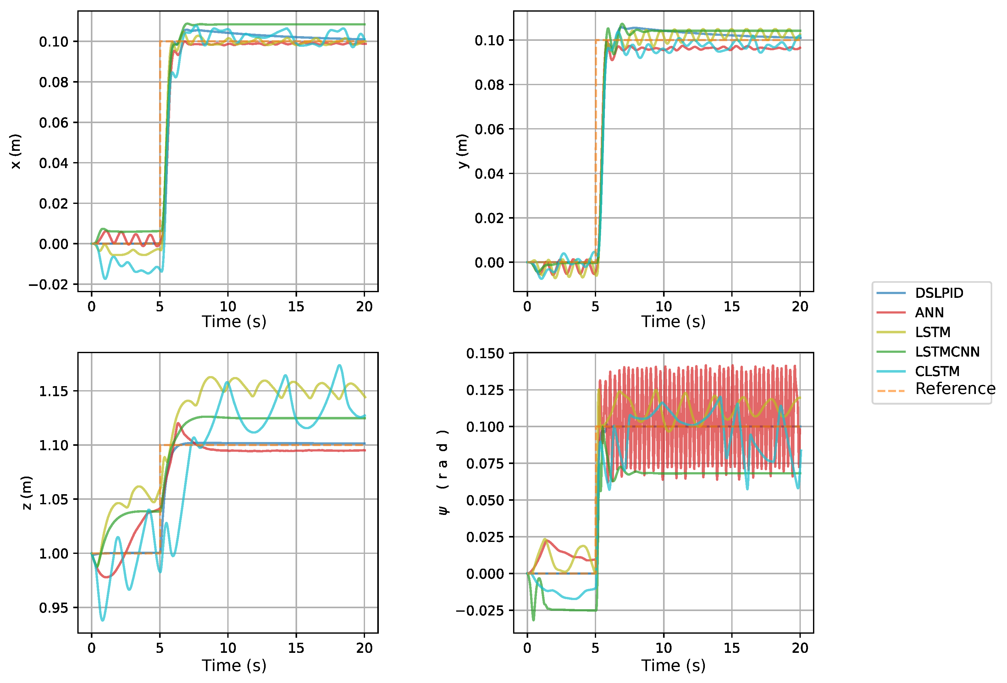
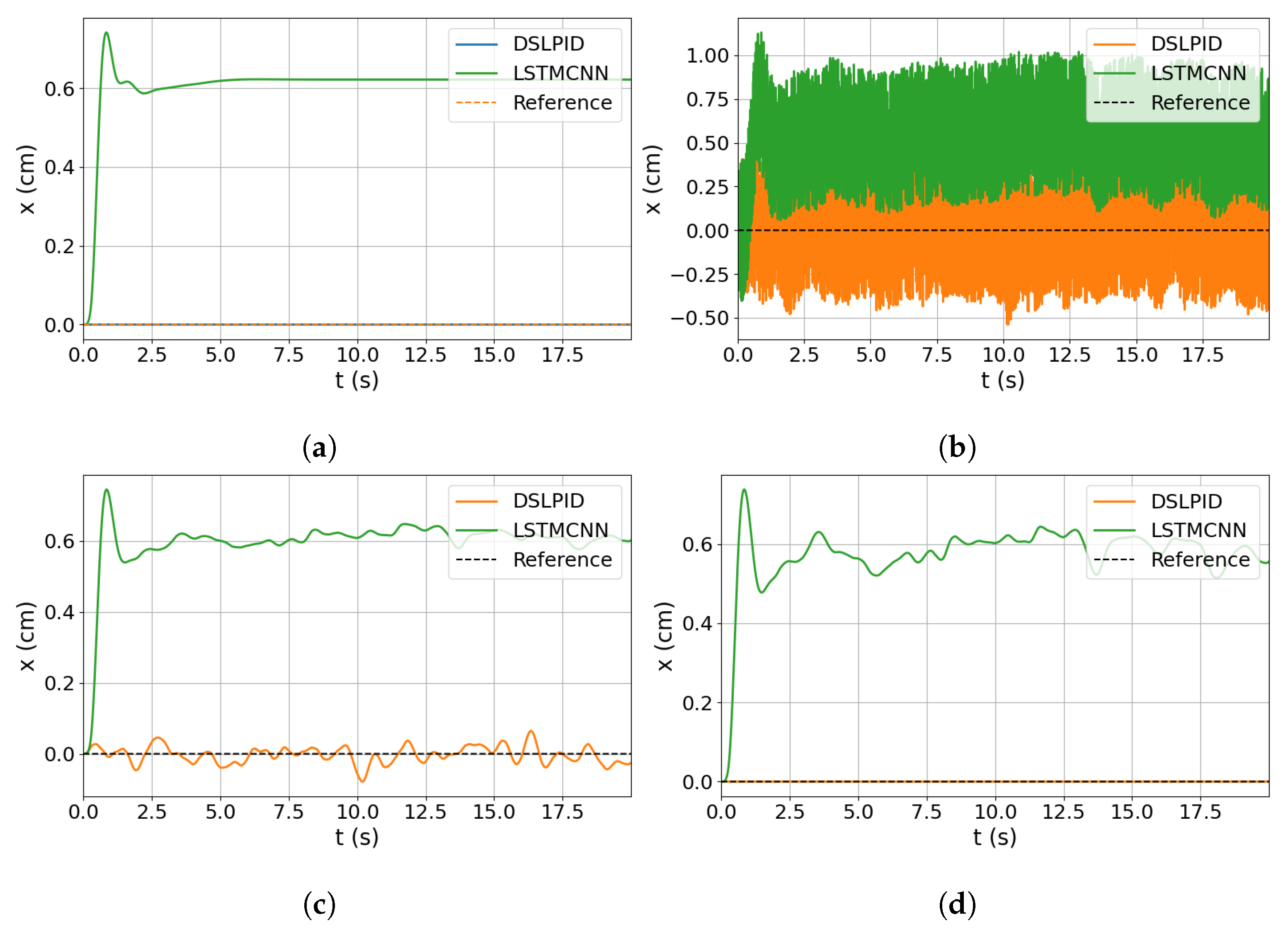
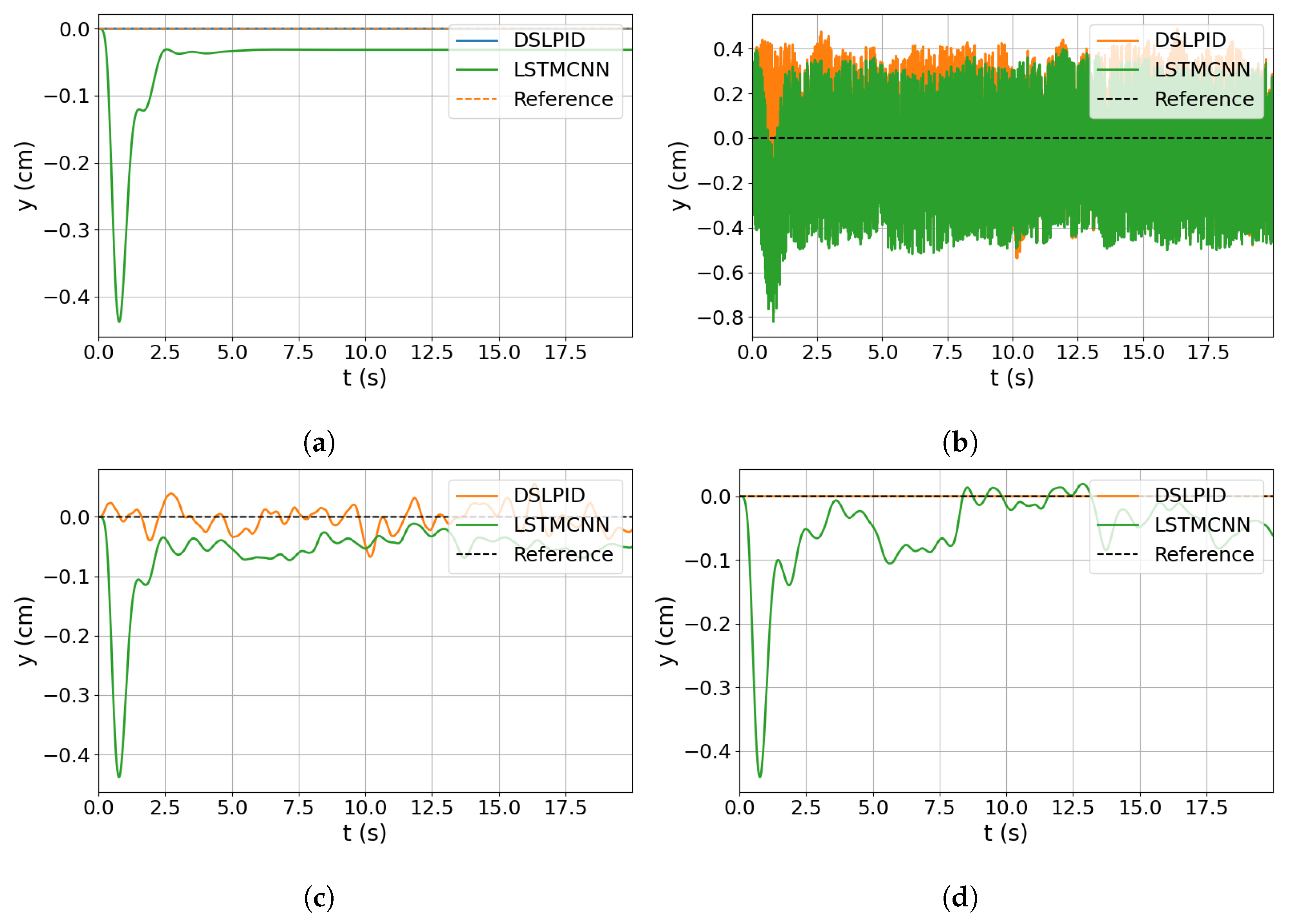
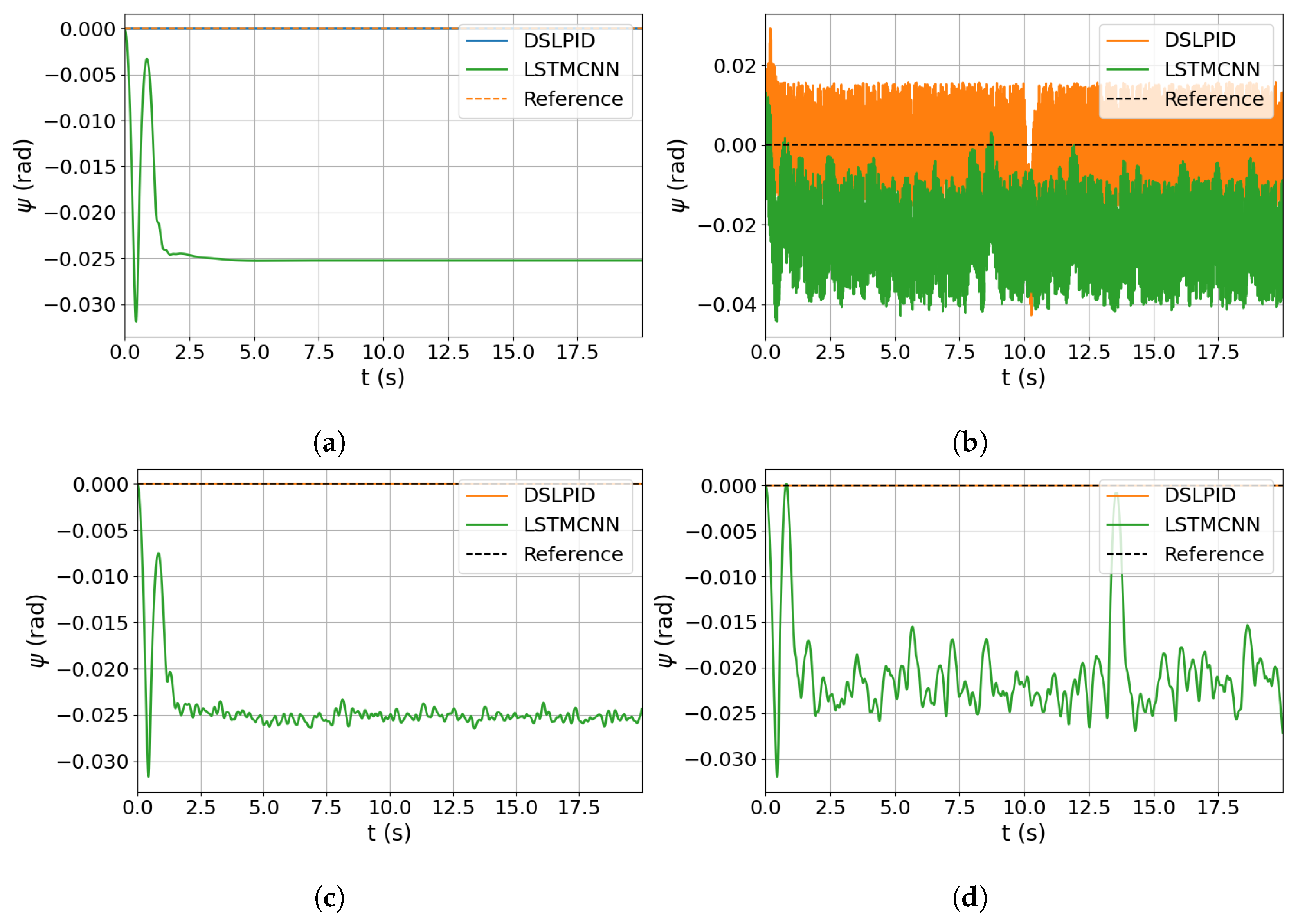
Regarding the step response experiment (Section 4.3.1), our controller exhibited similar responses to the baseline controller in the X and Y axes, accurately following the set point and maintaining stability. However, it showed higher steady-state error compared to the baseline controller in the $\psi$ and Z axes. The $\psi$ axis was particularly challenging due to the discontinuity of the state bounded between [$-\pi$; $\pi$].

Figure 13 depicts the control effort related to the stepping trajectory. The experiments indicate that our controller reduces the control effort required compared to the baseline controller.

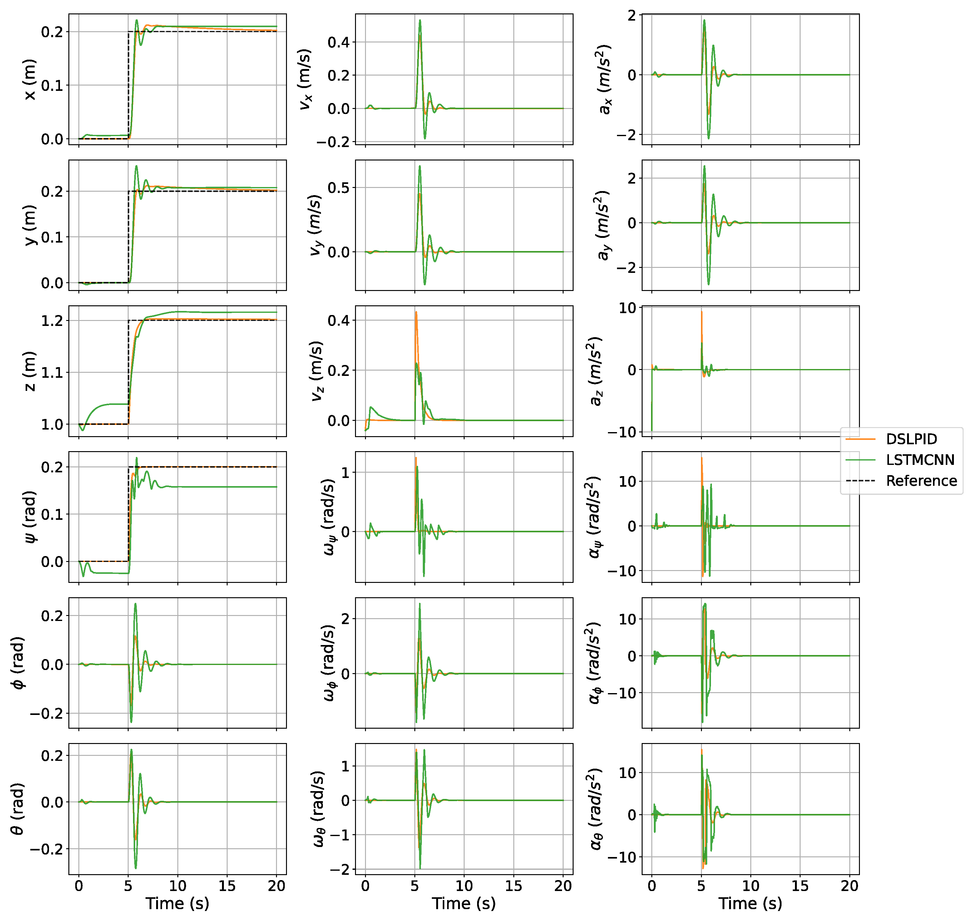
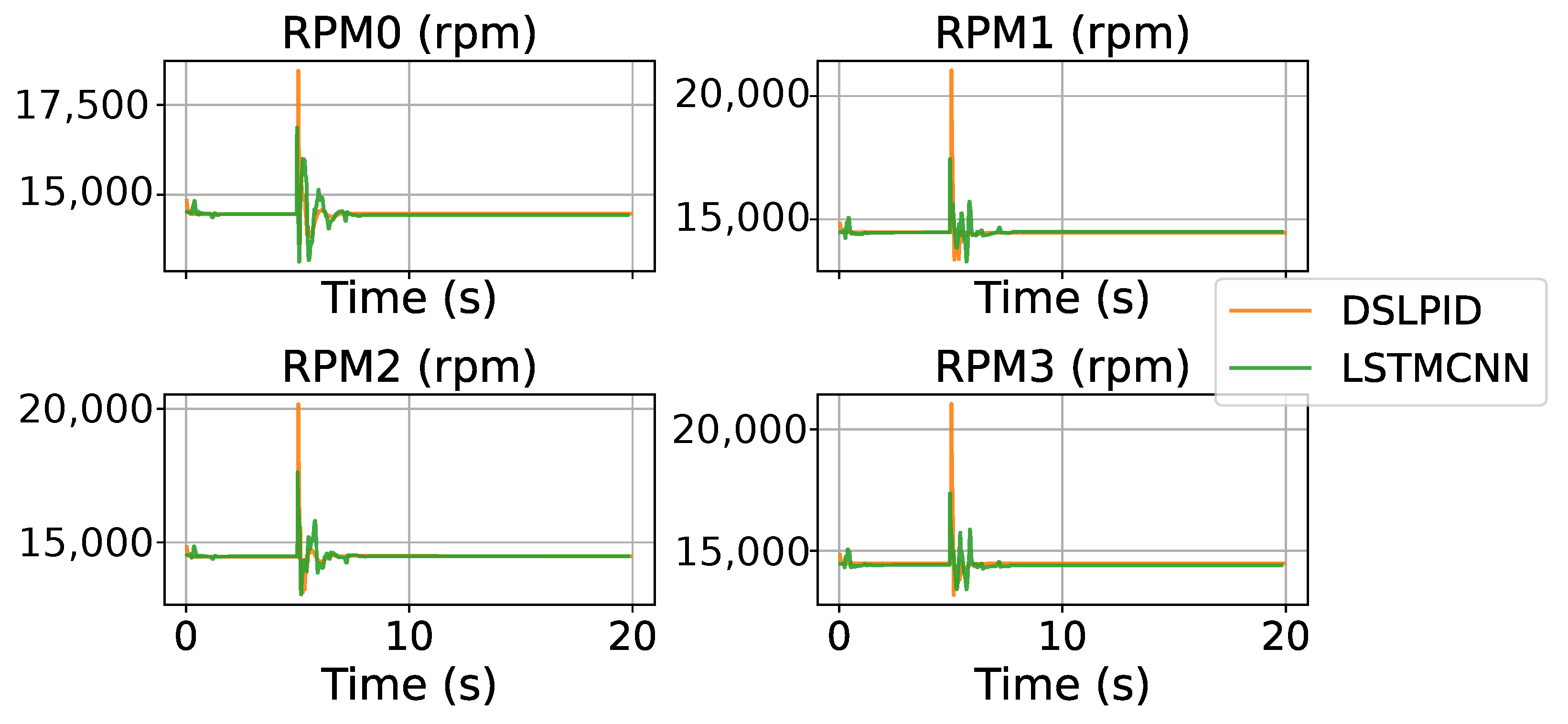
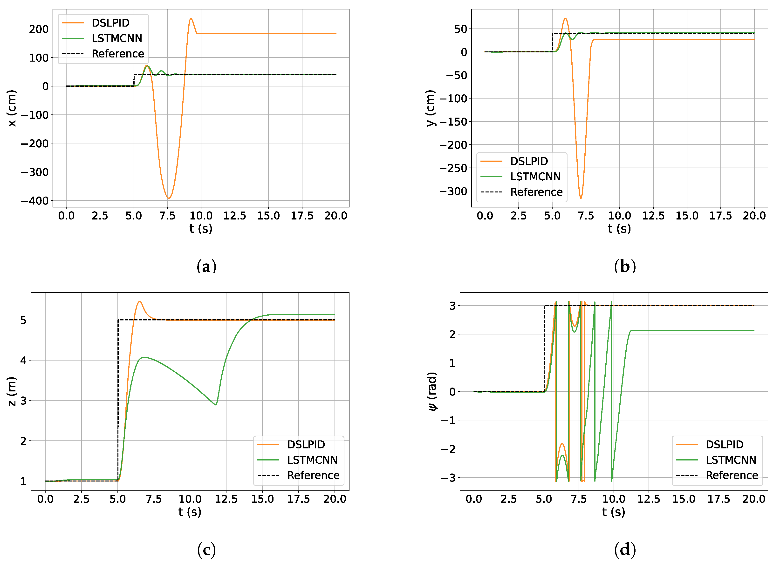
The results of the big-step experiment (Section 4.3.2) demonstrated that the LSTMCNN controller exhibited stability over a wider range of control beyond the nominal operating point in the x and y axes. This indicates its capability to accurately track and control the drone’s position even when subjected to larger step inputs. However, improvements are needed in the z axis and especially in the $\psi$ axis, where the LSTMCNN controller showed instability. Fine-tuning of controller parameters or architecture may be necessary to enhance performance in these specific axes.

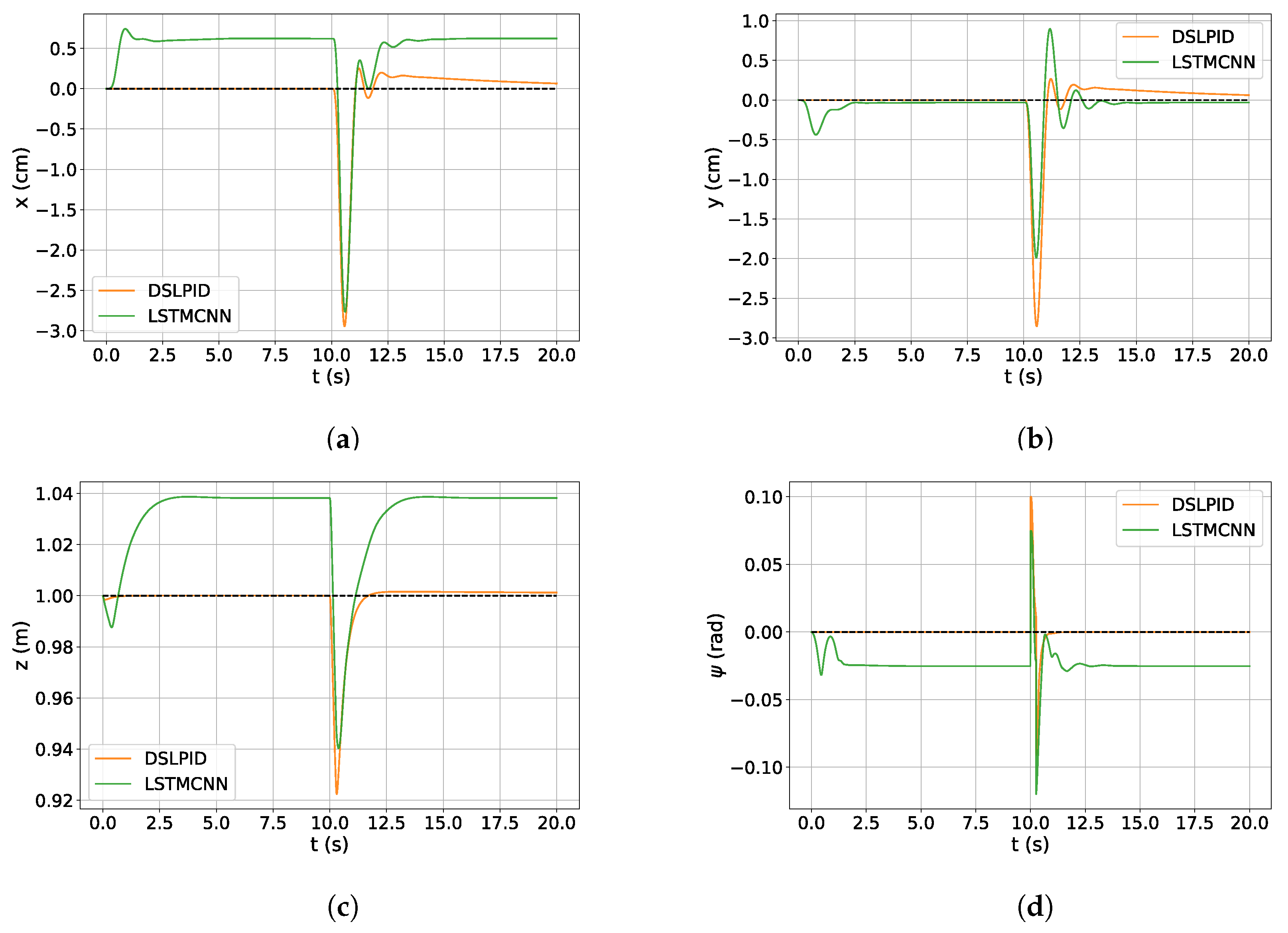
In the disturbance rejection experiment (Section 4.3.3), both controllers maintained stability in the presence of sudden disturbances. However, the DSLPID controller outperformed the LSTMCNN controller based on metrics such as settling time, overshoot, and steady-state error.

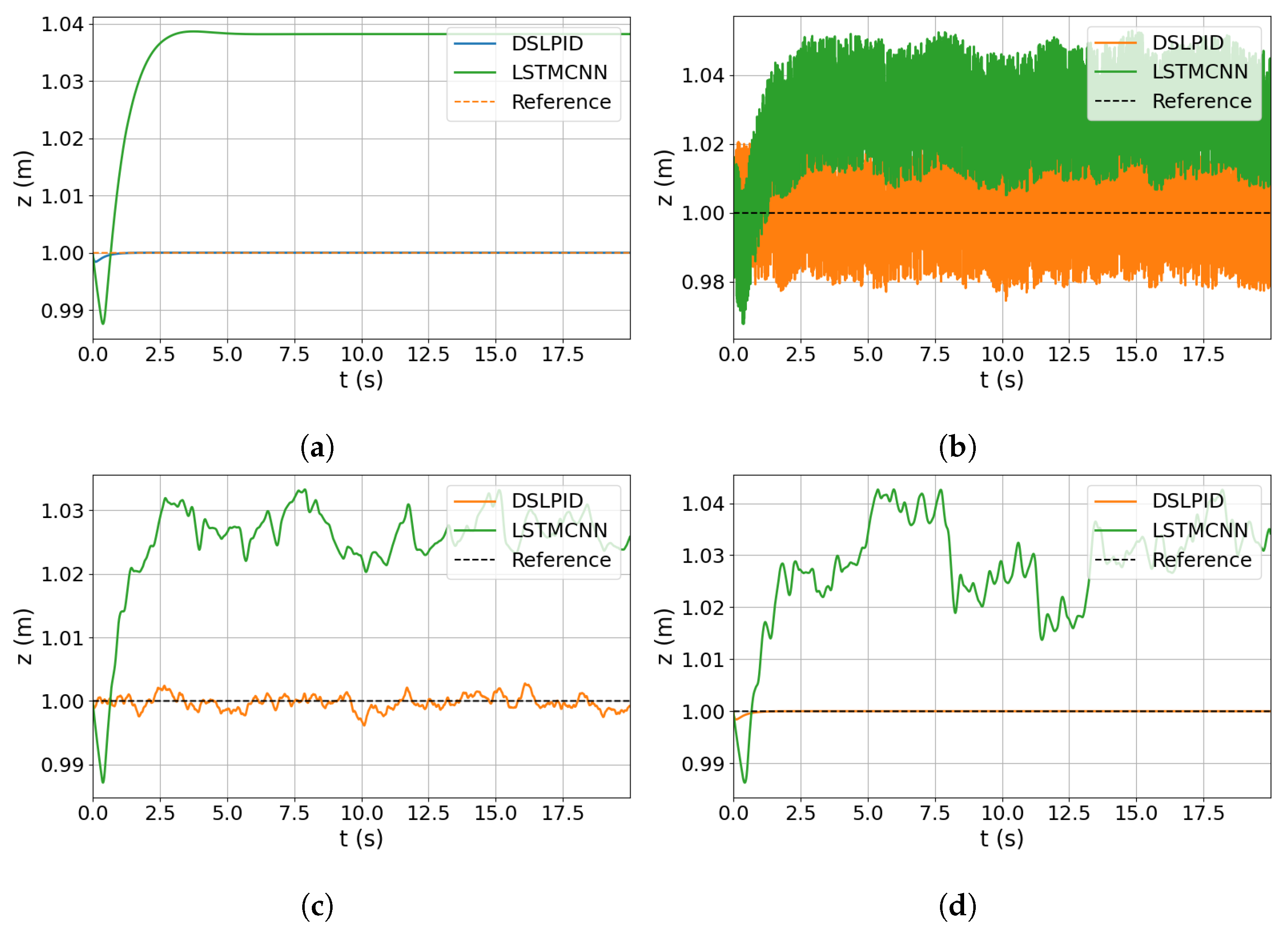
Contrary to our initial expectations, the noise degradation experiment (Section 4.3.4) revealed that the LSTMCNN Neural Network Controller exhibited increased sensitivity to noise, particularly when it affected the position variable. This highlights the challenges associated with noise in Neural Network Controllers and suggests the need for further investigation and improvements in architecture and training strategies to enhance noise robustness. The inclusion of acceleration information in the neural network’s predictions offers better generalization capabilities but also increases sensitivity to noise due to additional variables.

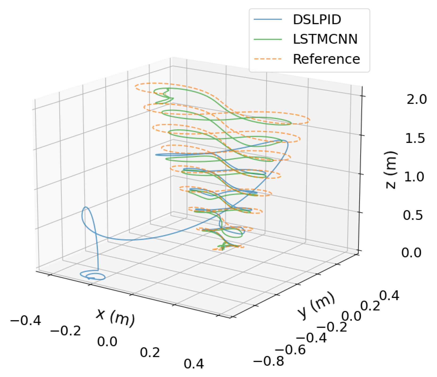
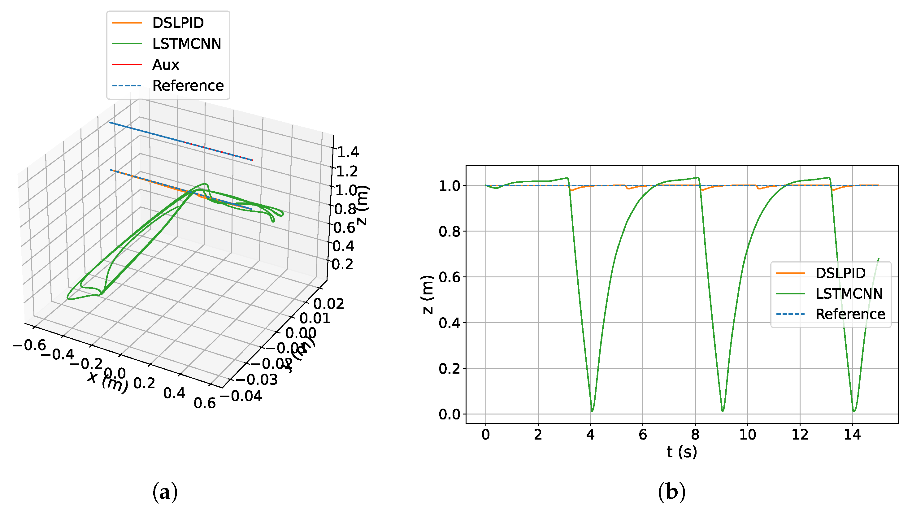
In the Lemniscate experiment (Section 4.3.5), the LSTMCNN Neural Network Controller successfully tracked the intricate shape of the Lemniscate function, showcasing its ability to handle demanding trajectories. Conversely, the baseline DSLPID controller struggled to follow the desired trajectory, leading to eventual instability accurately. These findings underscore the superior performance and robustness of the LSTMCNN controller in challenging scenarios involving aggressive set-points with high accelerations or large attitude angles.

When subjected to the downwash effect (Section 4.3.6), an aerodynamic phenomenon absent in the initial dataset, our model demonstrated limited adaptability. Although it maintained stability, the controller’s performance declined. To address this issue, retraining the controller with a more comprehensive dataset incorporating a wider range of aerodynamic scenarios could enhance its ability to handle the downwash effect and related factors. Alternatively, integrating online learning techniques into the controller’s architecture could enable continuous adaptation to real-time feedback and varying aerodynamic conditions. Further research and experimentation are necessary to determine the most suitable approach, considering factors such as resource availability, performance requirements, and feasibility within the specific problem context.

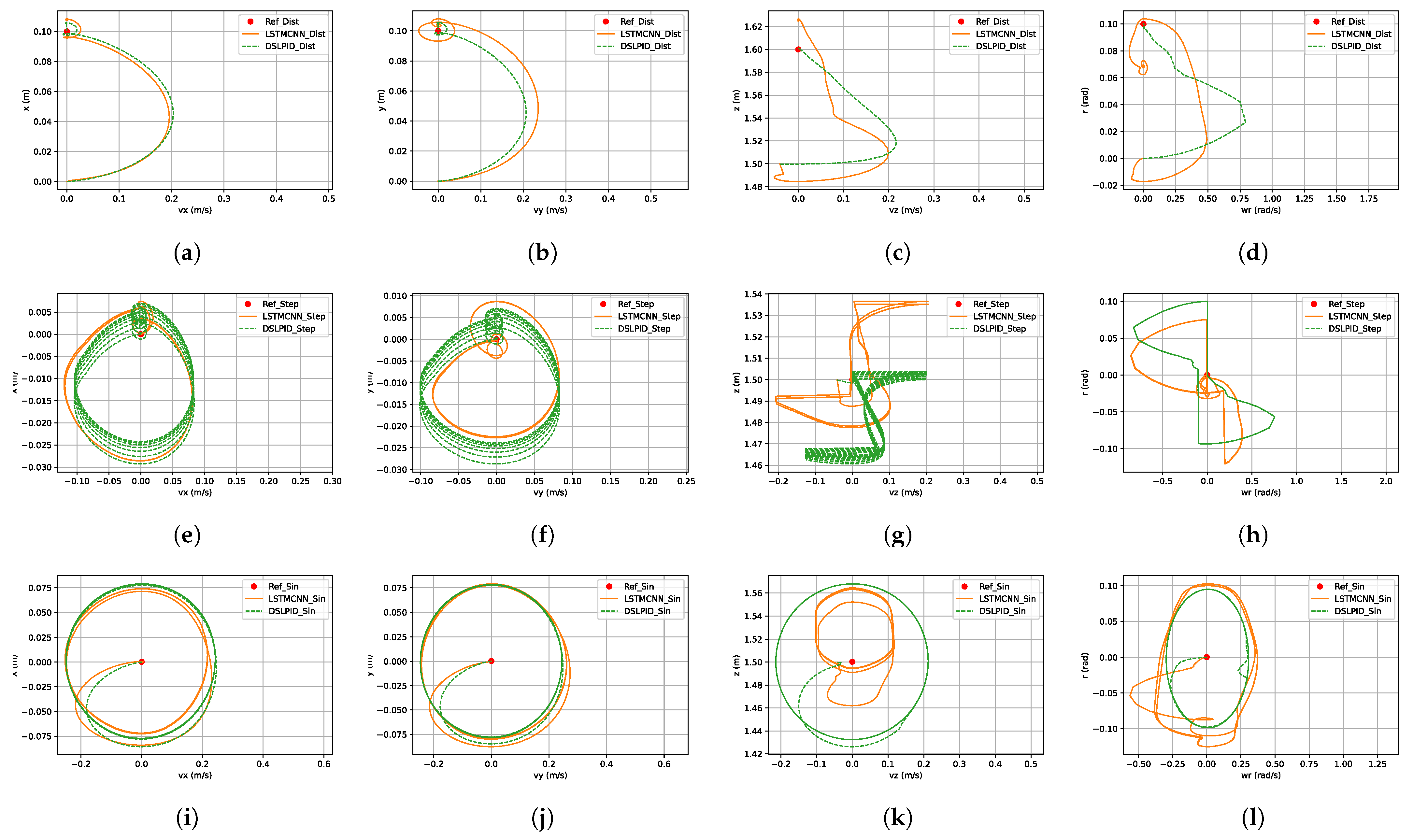
Lastly, the phase plane diagram in Figure 22 illustrates the stability of our controller within and beyond the operating point of the baseline controller. This analysis provides valuable insights into the behavior of the system’s state variables and supports the assessment of controller performance.

Overall, our study contributes to the broader understanding of neural network-based controllers for drone position control by providing insights into the strengths, limitations, and areas for improvement of such approaches. We highlight the trade-offs between different architectures and the challenges associated with noise sensitivity, aggressive trajectories, and the impact of aerodynamic effects. These findings can guide future research and inform the development of more robust and adaptable control strategies.

6. Conclusions

In this paper, we proposed a new flight control system implemented with Pybullet and its model for the Craziflie quadrotor. Our controller was developed based on the training and building of several Neural Network architectures proposed in the literature. These architectures were trained with data gathered by flying with the controller offered by Pybullet. Finally, our controller was evaluated in comparison with the controller offered by Pybullet. From this, we can conclude:

From our experiments, we conclude that the LSTMCNN architecture offers the best performance for controlling the Craziflie quadrotor. The best way to obtain this architecture’s parameters was by using the Hyperband algorithm and its time window by applying the partial autocorrelation function in combination with our proposed empirical method, which involved gathering data from flying with the Pybullet controller. Our empirical stability evaluation of the proposed controller architecture, as shown in Figure 22, demonstrates that it converges to the set-point in all axes for all evaluated trajectories.

From the proposed dataset, we found out that the signals that offer better information in terms of controller dynamics are the signals null with disturbances, low-frequency noise, and staggered random steps. These signals offer more information in terms of harmonic components.

Overall, this project provides a viable and reliable way to develop UAV flight neural controllers. The proposed Offline-Training approach enables the development of intelligent flight controllers in a more efficient manner than other proposals that might be implemented with Online-Training. We believe that these observations and conclusions offer important details for researchers and developers to take into account when gathering, training, and evaluating intelligent flight controllers.

7. Future Work

This work offers a broad landscape for future implementations of neural controllers for UAVs. For future offline training, we recommend training recurrent models for flight control by using the most realistic engine physics available to gather data, thereby providing more robustness. Our controller remained stable during testing, but we found that it was unsuitable for non-explored aerodynamic effects (Section 4.3.6).

Moreover, we propose implementing our best model within an online training algorithm with Pybullet, such as deep Q-network (DQN), deep deterministic policy gradient (DDPG), or advantage actor–critic (A2C), utilizing our developed open-source library for simulating neural controllers. To enhance the main trouble for our controller, which is the steady-state error, we recommend implementing a loss function that considers the accumulated error with the set-point signal and the basic control evaluation parameters (such as the customized function F1 for evaluating controller performance).

It is important to acknowledge that relying solely on offline training is unlikely to address these details, as supervised learning theory suggests that the behavior of our neural controller will be limited to replicating the proficiency of the sample controller at best. By embracing our proposed future work and incorporating online training algorithms, we aim to optimize the neural controller to exhibit the best behavior based on the defined loss function rather than merely imitating the behavior of a sample controller.

This future work proposal, where we implement our model within an online training algorithm, is motivated by the potential to save time and computational resources in developing a proficient flight neural controller. Research suggests that achieving complex behaviors such as stable flight control in a UAV through online training alone can be a slow process. Therefore, leveraging the existing convergence capability of our neural controller towards set points during flight can facilitate a more efficient online training experience, enabling us to refine control details and further enhance the performance of the neural controller.