Pose Determination System for a Serial Robot Manipulator Based on Artificial Neural Networks

Abstract

Achieving the highest levels of repeatability and precision, especially in robot manipulators applied in automation manufacturing, is a practical pose-recognition problem in robotics. Deviations from nominal robot geometry could produce substantial errors at the end effector, which can be more than 0.5 inches for a 6 ft robot arm. In this research, a pose-recognition system is developed for estimating the position of each robot joint and end-effector pose using image processing. To generate the joint angle, the system is developed via the modeling of a pose obtained by combining a convolutional neural network (CNN) and a multi-layer perceptron network (MLP). The CNN categorizes the input image generated by a remote monocular camera and generates a classification probability vector. The MLP generates a multiple linear regression model based on the probability vector generated by a CNN and describes the values of each joint angle. The proposed model is compared with the P-n-Perspective problem-solving method, which is based on marker tracking using ArUco markers and the encoder values. The system was verified using a robot manipulator with four degrees of freedom. Additionally, the proposed method exhibits superior performance in terms of joint-by-joint error, with an absolute error that is three units less than that of the computer vision method. Furthermore, when evaluating the end-effector pose, the proposed method showed a lower average standard deviation of 9mm compared with the computer vision method, which had a standard deviation of 13 mm.

1. Introduction

Reaching the highest levels of repeatability and precision for pose determination in robotic manipulators in automated manufacturing is currently a practical problem [1]. Even slight deviations from nominal robot geometry can produce substantial errors at the end effector, which can be greater than 0.5 inches at the end effector of a 6 ft robot arm. These errors occur due to a lack of stiffness, gear wear, encoder failure, etc. [2]. On manipulator startup, the system assumes that the manipulator’s joints are in the same angular position as they were on shutdown, which is not necessarily true due to malfunctions in incremental rotary encoders [3]. Robots are calibrated using laser probes and stereo cameras, and a specialized setup is necessary. This kind of process requires time stops for reprogramming, has high maintenance costs, etc. This paper proposes a pose-determination system throughout computer vision, which could provide auxiliary joint angle measurement in addition to encoders or other sensors, including robotic systems to help increase accuracy or even reduce encoders cost. In other cases, a pose-determination system can be used as an auxiliary method to prevent accidents by determining the robot pose, which interacts with the working environment.

In workspace determination, for example, the authors of [4,5] use the technique to isolate the singularities output and generate a detailed map of the workspace or even a force-closure condition specifically in the end-effector pose.

Pose-estimation applications combined with sensors, such as vision sensors, in addition to encoders, are widely used. For example, stereo cameras are used as vision sensors [6] in machine learning applications [7] to measure spatial dimensions [8,9,10] and are also used in areas such as autonomous navigation [11,12] and aerospace engineering [13]. In general terms, stereo cameras can obtain pose measurements in a complex environment [14], as well as poses based on a real-time view of the non-cooperative target using the extended Kalman filter [15]; monocular vision systems for the online pose measurement of a planar manipulator [16]; autonomous charging applications using visual guidance [17]; pose measurements based on a monocular camera mounted on a robot manipulator that estimates pose parameters using a feature point [18]; convenient pose measurements using Monte Carlo localization with the scan matching method [19]; or practical applications, such as a system based on a camera hung from the ceiling facing toward the ground [20].

Various systems have been developed for flexible pose-estimation applications, including using markerless options combined with artificial intelligence [21], fixed cameras in the scene with marker colors [2], tree marks and colors [22], and applications with deep learning and Kalman filters [23]. Driels et al. [24] reported a method for the kinematic calibration of a robot manipulator using a coordinate measuring machine (CMM), which can obtain the end effector’s whole pose. Driels and Swayze [25] published work concerned with methods that provide partial pose data for robot calibration tests. Rather than focus on traditional precision measurement techniques, the paper discusses calibration using various endpoint motion constraints. Bai and Yeong Teo [26] developed a calibration method utilizing base and tool transformation under optical position sensors. Meng and Zhuang [27] published a vision-based self-calibration method for a serial robot manipulator that only requires a ground-truth scale in the reference frame. In [28], they propose a new calibration method for a 5-Degrees-Of-Freedom (DOF) hybrid robot, concentrating particularly on addressing the contradiction between measurement efficiency and calibration accuracy, and real-time compensation with high precision. The approach involves two successive steps: (1) an error-prediction model based on a back-propagation neural network (BPNN) combined with the Denavit–Hartenberg (D-H) method established by the pose error decomposition strategy; and (2) an embedded joint error compensator based on a BPNN designed to achieve real-time compensation with high precision. In [29], they describe the development of a calibration procedure for a 5-DOF serial robot using a laser tracker. The main goal of this paper is to utilize measurements relative to the robot’s end effector to compensate for errors. The robot kinematic model is computed to help identify the deviations. Robot parameter deviations can be identified so that the nominal parameters can be corrected.

Control pose is an active topic related to pose determination or estimation, and systems have been developed that use cameras to locate the position of robotics platforms [30], including an uncalibrated eye-in-hand vision system to provide visual information for controlling the manipulator mounted on the mobile base [31], the robot visual servo positioning control and insulated wrapping manipulator of a distribution line [32], and applications in medical environments [33]. Related to the control pose in industrial robots [34], robot controller delay is proposed, and robot dynamics are identified as the key missing components, with a new data-driven method for capturing the robot dynamics and a model for closed-loop stability prediction being established. The new model-based method is experimentally evaluated on a 6-DOF industrial manipulator.

A summary of other computer vision pose-estimation applications are described as follows: in [35], they proposed a computer vision system that estimates the pose parameters (including orientation and position) of the excavator manipulator. To simulate the pose-estimation process, a measurement system was established with a common camera and marker. In [3], the authors proposed a system comprising a SCARA manipulator, a Raspberry Pi camera, a fish eye lens, and colored markers (painted spheres), which was able to estimate joint angles with some errors. For marker tracking, a Kalman filter and particle filter were combined and used to estimate homography matrix world coordinates. In [2], they utilize machine vision, with a single camera fixed away from the base of the manipulator using markers placed on each joint. Based on a single instant image, the kinematics of the manipulator, and the calibrated camera, the pose of the manipulator can be determined. However, this approach cannot compete with encoders and is restricted by deployed equipment.

The theoretical perspective of the literature review shows that there are a few publications related to the pose determination of serial robots using a single camera in a fixed scenario; however, they are poor exceptions that are not robust to the occlusion of some movement trajectories in the pose-determination process. This work considers a scenario where the robot and a monocular camera are situated in a fixed position away from the manipulator and placed in a frontal view perspective, where pose determination is required that considers worse conditions than those expressed in the literature review and that can combine the strengths of different areas, such as computer vision and artificial intelligence, achieving flexible system implementation.

The proposed approach estimates the manipulator pose using visual information provided by a single camera without the use of markers on each joint, and it is robust to changes in environmental light conditions with a few adjustments. This research has been motivated because of current problems in automotive assembly. This application can be used for assembly tasks within the automotive industry, making programming more flexible and accounting for a considerable variety of objects with different geometries. Furthermore, the fact that our proposed method does not depend on a particular robust graphic marker or specific color marker makes it robust to light changes and the wide variety of the object designs produced, thus facilitating its application in other programmable machines in which having flexible tools positioning is crucial.

The contribution of this research is a pose-recognition system for determining the joint angles of a robust serial robot for use in different light conditions and with different models of robot arms, which, combined with forward kinematics, can estimate the pose of the serial robot’s end effector. The proposed model is oriented as a backup system when encoders fail during task execution. Combined with the information from encoders, pose determination could lead to a more stable pose by using the model as a reference with the kinematic control of each joint, establishing a flexible method of reprogramming tasks during industrial operations. The proposed system is based on pose modeling obtained from the development of a convolutional neural network (CNN) combined with a multi-layer perceptron network (MLP) to generate the joint angle. The CNN classifies the input image and generates a classification probability vector. The MLP generates a multiple linear regression model based on the probability vector generated by the CNN and describes the values of each joint angle. As a measure of the system’s feasibility, this is compared with the ground-truth values obtained from the robot’s encoders, and it is compared with the Perspective-n-Point (PnP) features points position using ArUcos markers and a calibrated camera, which is used to obtain 3D homogeneous coordinates and the rotation matrix to establish the pose. Furthermore, the experimental results of different poses are calculated via the new approach and confirmed using an analytical solution, and the estimation error is calculated to demonstrate the effectiveness of this new approach.

This research paper is organized as follows: Section 2 describes the architecture of our proposed approach. Section 3 explores pose estimation by Perspective n Point (PnP). Section 4 presents the experimental results of the system’s implementation on the robot manipulator. Section 5 provides a discussion, and Section 6 presents our conclusions and proposed future work.

2. Proposed System Approach

The proposed system is based on monocular vision, where a camera captures the movement of each joint, and the resulting images are processed using a combination of a CNN network and an MLP network. In the CNN stage, the system generates a classification vector, which serves as input for an MLP network that can generate an angle value for each joint based on the image input. To ensure the system’s proper functioning, a training phase is required for each stage. This leads to a robust system that can handle variations in the pose and can be deployed on simpler hardware once trained. The proposed pose-recognition system is enumerated as follows and shown in Figure 1.

2.1. Proposed Convolutional Neural Network

It is widely known that CNNs are used in a vast majority of image classification tasks with acceptable performance. This robust neural network performs feature extraction from an image streaming source, and then the characteristic features are used to estimate convolutions and poolings along all of the networks to obtain an output that is interpreted by a dense neural network generating a set of probabilities assigned to the input classified.

CNNs have multi-dimensional and special layers called convolutional layers and pooling layers, which help reduce the size of the convolved features detected by image analysis. Convolutional layers have different dimensions, for example, one-dimensional layers are used for sequences of data, and two-dimensional layers are used for image analysis. Inside a convolutional layer, a convolution is developed. On this, there is an input layer; a kernel; and an output layer, which describes the convolved feature of the input.

For better performance, a CNN design comprising multiple convolutional layers combined with pooling layers to improve the network is recommended.

Once the convolutional features are obtained through a set of convolutional and pooling layers, these are passed by a flattening process, which implies a conversion of a one-dimensional vector as an input vector of a feed-forward network. This type of network requires several training phases to achieve optimal weights and biases for proper image classification. The proposed model is designed to classify a set of different RGB images from measurements that vary from the poses of the robot, which are established as 15 degrees of increment per joint. The detailed summary of the network is shown in

Table 1. Artificial neural network architectures. The parameters involved in the combination of the CNN and MLP models.

	Layer (Type)	Output Shape	Param #
	2D-Convolutional-Layer-1	(None, 126, 126, 16)	448
	(Conv2D)
	2D-MaxPool-Layer-1	(None, 63, 63, 16)	0
	(MaxPooling2D)
	Dropout-Layer-1 (Dropout)	(None, 63, 63, 16)	0
	2D-Convolutional-Layer-2	(None, 61, 61, 64)	9280
	(Conv2D)
	2D-MaxPool-Layer-2	(None, 30, 30, 64)	0
	(MaxPooling2D)
CNN Model	Dropout-Layer-2 (Dropout)	(None, 30, 30, 64)	0
	2D-Convolutional-Layer-3	(None, 30, 30, 64)	36,928
	(Conv2D)
	2D-MaxPool-Layer-3	(None, 15, 15, 64)	0
	(MaxPooling2D)
	Dropout-Layer-3 (Dropout)	(None, 15, 15, 64)	0
	Flatten-Layer (Flatten)	(None, 14,400)	0
	Hidden-Layer-1 (Dense)	(None, 64)	921,664
	Output-Layer (Dense)	(None, 12)	780
	Dense (Dense)	(None, 6)	78
MLP Model	Dense_1 (Dense)	(None, 8)	56
	Dense_2 (Dense)	(None, 1)	9

.

This CNN was trained using an image data set of different poses along a group of trajectories. The RGB image input size was 128 × 128 × 3 pixels.

2.2. Proposed Linear Regression Model Based on Multilayer Perceptron Network

An MLP network is a feed-forward artificial neural network. These are used to describe networks comprising multiple layers of perceptrons. A perceptron is a basic unit of a neural network that simulates a biological neuron. These consist of at least three layers of nodes: the first layer is the input layer, the middle layer is known as the hidden layer, and there is also an output layer. All of the nodes use a nonlinear activation function, except for input perceptrons, which are provided by the input data from the training data set. A neuron can be expressed as:

$${\displaystyle r_j=f\left(a_j\right)=f(\sum _{i=0}^d{w}_{ji},s_i)}$$

(1)

where d expresses the d-dimensional input vector, s and $r_j$ are the output vector, and $w_{ji}$ denotes the weight between output neuron j and input neuron i. In the case of the function, f is used as the activation function, and this is nonlinear.

The use of MLPs as multiple regression models (MLR) is a well-studied topic. The proposed MLP is used to estimate the values of each joint’s manipulator angles, which do not depend on any specific orientation.

Once the CNN estimates the probability vector of the input image, the MLP is designed to use these values and estimates the value of each joint’s manipulator angle. Table 1 shows a summary of the proposed system.

The CNN and the MLP were trained separately. The CNN was trained using the cross-entropy function describing a typical training loss classification task. Once trained, the CNN was used to generate a set of probability values for each image according to the value of each joint’s angle position on the manipulator, thus obtaining a set of data for the MLP training process related to the CNN training process.

2.3. Proposed Pose-Recognition System (CNN + MLR)

The proposed system is described as shown in Figure 1. It is a combination of a CNN and MLP used as a multi-linear regression model for each joint angle. First, the system can be used as an alternative to encoders or as a robust option for tracking and recognizing the pose of a robot manipulator.

The system uses an image that can be obtained from a video image stream as an input. Once the CNN is trained, it can classify a pose between a group of different classes. Each class has a predictive value that describes the category and is related to the value of the robot placement and the angle value of each joint.

The values of each class probability are then used as parameters of the multi-linear regression model generated by the MLP network, which a priori was trained and can generate estimated values for each joint angle, and it can be implemented with forward kinematics to establish the robot’s pose based on an image.

The system’s output is the angle of each robot joint, which can be used to determine the pose of the end effector.

This method is more robust than others such as Perspective n Point because it does not depend on a specific marker [35] or need specific light conditions [3]. Moreover, this method can be used in circumstances where the robot is partially occluded, with promising results.

2.4. Classes Generated by Joint Angles

Trajectories were developed using each joint separately for the free movement of the envelope. The joint movement was captured by a camera after periods of 1 s and 15 degrees of movement. The selection of angle size is determined according to

Table 2. Class angle determination.

Angle Size (Step) (Degrees)	Training Time (Min)	Error Estimation Compared with Encoder Signal	Number of Images in Data Set
20	25.8	3.89	2925
15	32.1	1.30	3250
10	51.9	0.91	5525
5	96.6	0.75	7400

, which shows the best performance at 15 degrees based on training time and the number of images. On each joint, the trajectory starts at 0 degrees of the joint motor and increases until it reaches the joint limit.

2.4.1. Data Set for CNN Classification

The classification data set for the CNN was developed from video streaming. The data set is composed of 10,050 images of 1920 × 780 × 3 pixels. These were divided by using 80% for the training process, 20% for the validation process, and 300 additional images for the testing process, which we did not use for the classification pose’s training and validation tasks.

2.4.2. Data Set for MLP Fitting as MLR

The data set of the MLP fitting as the MLR was developed by utilizing the images previously used in the latter stage of classification using the CNN. The training images are used in the CNN to obtain a vector of class probability; then, these values are stored to create a data set for MLP training, where the input data of the MLP are the probabilities of each pose, which are related to the joint angle measured by the encoders. The target values of the data set are the ground-truth values of each joint at the time when the image is captured. The arrangement of the values for training, validation, and testing was the same as that used by the CNN classification process.

2.5. Evaluation Metrics for the Proposed System Evaluation

The proposed system is evaluated separately. For one part, a set of metrics is used to evaluate the performance of the CNN, and for the other, an MLR is used to determine metrics such as mean square error, mean absolute error, and $R^2$.

2.5.1. Performance Evaluation of CNN

In the context of the classification models, a confusion matrix is a table that summarizes the performance of a classification algorithm by displaying its actual and predicted results. It contains four elements that describe the performance: true positives (TP), true negatives (TN), false positives (FP), and false negatives (FN). The F-Score is the harmonic mean of precision and recall and provides an indication of how precise the classifier is. A high F-Score value indicates that the model performs better in positive cases. The sample size is denoted by N. A comprehensive description of the relationship between these parameters and a confusion matrix can be found in [36].

The parameters to establish the performance of the CNN are accuracy, precision, recall, and F-Score, which are estimated as shown below:

$$Accuracy=(TP+FN)/N$$

(2)

$$Precision=TP/(TP+FP)$$

(3)

$$Recall=TP/(TP+FN)$$

(4)

$$F-Score=(2\times Precision\times Recall)/(Precision+Recall)$$

(5)

2.5.2. Performance Evaluation of MLR

The first parameter is the mean square error (MSE), which is the difference between the ground-truth values and the predicted values squared by the mean difference. This can be expressed as

$$MSE=\frac{{\sum }_{i=1}^N{(true\_valu{e}_i-predicted\_valu{e}_i)}^2}{N}$$

(6)

The second parameter used as a metric of performance is the mean absolute error (MAE), which establishes a difference between the original values and the predicted values. This can be expressed as:

$$MAE=\frac{{\sum }_{i=1}^{N}abs(true\_valu{e}_i-predicted\_valu{e}_i)}{N}$$

(7)

Another parameter is $R^2$, which established how well the values fit compared with the original values. This can be expressed as:

$$R^2=1-\frac{{\sum }_{i=1}^n(predicted\_valu{e}_i-mean\_value)}{{\sum }_{i=1}^n(true\_valu{e}_i-mean\_value)}$$

(8)

2.6. Manipulator Kinematics Analysis

The Denavit–Hartenberg (D-H) transformation matrices are commonly used to describe manipulator kinematics. The pose determination of the manipulator is created by establishing the D-H parameters. The obtained pose is confirmed by the encoders of each joint controller and verified by calculating the manipulator’s forward kinematics.

The robot arm is composed of the base, waist, upper arm, lower arm, and gripper. It has four degrees of freedom; the first three are revolute joints, and the fourth is a drive for the gripper position, as shown in Figure 2.

There are plenty of methods for a forward-kinematics estimation of a robot arm. Many of them are used to calculate rotation, such as Euler angles, Gibbs vectors, and others, but the most popular is the homogeneous transformation method. The matrices are used to define different Cartesian coordinate systems through the kinematic chain, which is based on rotation and translation matrices, as shown in [37]. The parameters are expressed in Figure 2.

x, y, and z refer to the rotating axes; $\theta$ is the rotating angle; and $c_{\theta }$ and $s_{\theta }$ represent cos$\theta$ and sen$\theta$, respectively.

The D-H convention exposes each coordinate frame on a link of a manipulator and the transformation from coordinate i−1 to i. ${\theta }_i$, $d_i$, $a_i$, and ${\alpha }_i$ are rotation in the Z axis, translation in the Z axis, translation in the X axis, and rotation in the X axis, respectively. The coordinate transformation matrix is expressed as:

$$=\left[\begin{array}{cc}{}^{i-1}{\overline{R}}_i& {}^{i-1}{\overline{P}}_i\\ 0& 1\end{array}\right]$$

(9)

where $\overline{R}$ and $\overline{P}$ are rotation and translation matrices from the previous link coordinate system to the next one, respectively, as mentioned in [38], and can be expressed as:

$${}^{i-1}{\overline{R}}_i=\left[\begin{array}{ccc}{c}_{{\theta }_i}& -c_{{\alpha }_i}{s}_{{\theta }_i}& s_{{\alpha }_i}{s}_{{\theta }_i}\\ s_{{\theta }_i}& c_{{\alpha }_i}{c}_{{\theta }_i}& -s_{{\alpha }_i}{c}_{{\theta }_i}\\ 0& s_{{\alpha }_i}& c_{{\alpha }_i}\end{array}\right]{,}^{i-1}{\overline{P}}_i=\left[\begin{array}{c}{a}_i{c}_{{\theta }_i}\\ a_i{c}_{{\theta }_i}\\ d_i\end{array}\right]$$

(10)

The D-H matrix is expressed as:

$${}^i{\overline{T}}_n=\left[\begin{array}{cccc}{r}_{11}& r_{12}& r_{13}& p_x\\ r_{21}& r_{22}& r_{23}& p_y\\ r_{31}& r_{32}& r_{33}& p_z\\ 0& 0& 0& 0\end{array}\right]$$

(11)

The final position of the end effector is denoted by ($p_x$, $p_y$, $p_z$).

3. Comparison with Pose Estimation by Perspective-n-Point (PnP)

The proposed comparison is established using the method presented in [35], which was selected because it displays a more robust performance than other computer vision methods applied as pose estimators.

Once camera calibration is established, the system determines the existence of characteristic features for each joint and estimates the x and y poses in the image, and then this is used to solve the PnP problem later, generating a translation vector with X, Y, and Z positions and a rotation vector of each marker. Furthermore, the rotation vector is converted as a rotation matrix using Rodrigues’ method [39], and then it is stored to convert the rotation matrix to Euler angles.

3.1. Parameters for PnP Problem Solving

The parameters to establish the comparison between the two methods are mainly expressed in the camera calibration parameters, ArUcos marker parameters, and algorithms to solve the PnP problem.

3.1.1. Camera Calibration

The camera calibration process, a matrix that is composed of intrinsic and extrinsic parameters, is presented mathematically, and it is related to the internal physical characteristics of the camera model as well as its position when taking the pictures, as based on [40]. This matrix is expressed as:

$$w\left[\begin{array}{c}x\\ y\\ 1\end{array}\right]=P\left[\begin{array}{c}X\\ Y\\ Z\\ 1\end{array}\right]$$

(12)

where w is the scale factor; x and y are the image’s homogeneous coordinates of the projected point in the image plane; X, Y, and Z are the homogeneous 3D point coordinates; and P is the camera matrix, which has intrinsic and extrinsic parameters, expressed as:

$$P=\left[\begin{array}{c}R\\ t\end{array}\right]K=\left[\begin{array}{ccc}{r}_1& r_2& r_3\\ & t\end{array}\right]K$$

(13)

$r_1$, $r_2$, and $r_3$ are the columns of the 3 × 3 rotation matrix R; t is the translation vector; and K expresses intrinsic and extrinsic parameters expressed as:

$$K=\left[\begin{array}{ccc}{f}_x& s& u_0\\ 0& \alpha f_x& v_0\\ 0& s& 1\end{array}\right]$$

(14)

where $f_x$ is the focal length corresponding to the x axis of the camera coordinates; $\alpha$ is the aspect ratio; s refers to the skew factor; and ${\left[u_0{v}_0\right]}^T$ is the principal point of camera. K can be simplified to only three parameters assuming unit aspect ratio and zero skew

$$K=\left[\begin{array}{ccc}f& 0& u_0\\ 0& f& v_0\\ 0& s& 1\end{array}\right]$$

(15)

f is the focal length and ${\left[u_0{v}_0\right]}^T$ is the principal point of the camera, as mentioned in [41].

This process is based on [42], which proposes that image calibration can be established while also allowing the establishment of a relationship between the physical world and the image plane.

The camera’s intrinsic and extrinsic parameters are needed to establish the pose of the markers mounted on the manipulator, and this can be achieved by camera calibration.

The camera calibration is performed using OpenCV based on the calibration method, and the camera parameters such as focal length, center point, and distortion coefficients are determined. For this purpose, a chessboard pattern with a grid of 8 × 8 squares is used. The camera that needs to be calibrated is used to take 20 pictures of the chessboard pattern from different perspectives.

The camera calibration parameters obtained are expressed as follows: intrinsic parameters ($f_x,f_y$ = [1014.3489, 1014.3489]), center point ($u_0,v_0$ = [640.00, 360.00]), and distortion coefficients ($k_1,k_2$ = [−0.318440, 0.171776]; $p_1,p_2$ =[−0.008577, 0.002376]).

3.1.2. ArUco Markers

The ArUco markers are used for pose estimation in several fields. They consist of a group of several synthetic square markers, which are made with a wide black border and an inner binary matrix that determines its identifier. The black border is used for detection in the image, and the image generated by the binary codification allows for its identification [43]. The marker size mounted in the robot is 10 × 10 mm, and it is placed on each joint and the end effector. The dictionary used for the binary image is 4 × 4 with 50 different designs.

Feature detection is established using an ArUco marker detector based on [43], and the markers are in Figure 3.

3.1.3. Solving PnP Pose Estimation

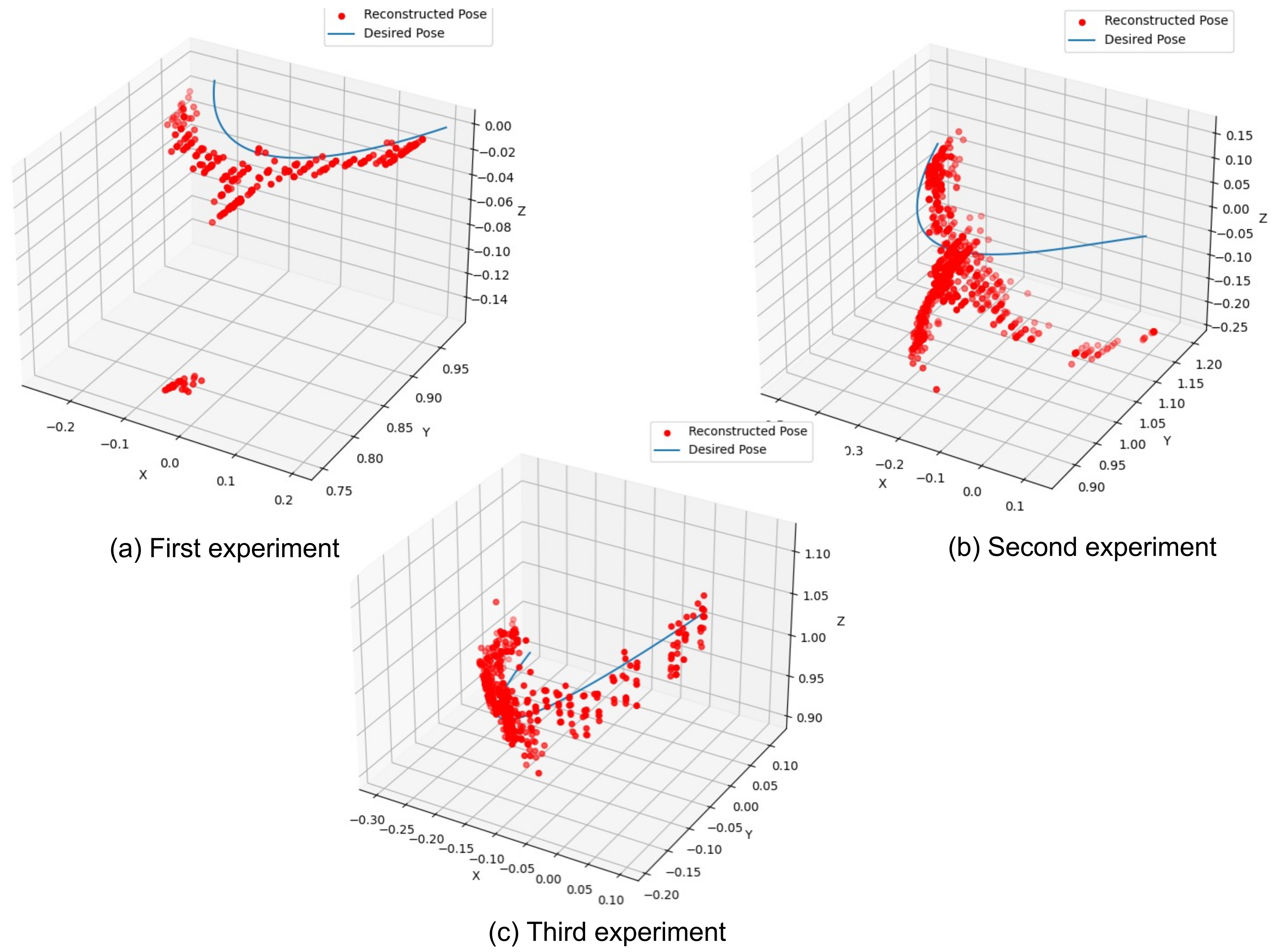
Once each feature is detected, the real-world position of the pattern is estimated. The way to convert from pixels to (X, Y, Z) coordinates is by solving the PnP problem as seen in Figure 4. The best solution is the combination of camera position and rotation, which makes the positions of the features as seen in the image.

To establish the intrinsic matrix and the distortion coefficients obtained from the calibration method, the coordinates of the pattern, which relate to the pixels position of the marker in the image and the pixels of the features in the image, are defined in the same order as in the previous section.

The pose is determined by reducing the reprojection error, which is described as:

$${\displaystyle \underset{R_i,t_i}{argmin}\sum _{i=1}^n\sum _{j=1}^m{\parallel \widehat{p}(K,R_i,t_i,P_j)-p_{ij}\parallel }^2}$$

(16)

where $\widehat{p}$$(K,R_i,t_i,P_j)$ is the projection of the P in the i-th image. These are solved using the optimization algorithm, as Levenberg–Marquardt as mentioned in [35].

4. Results

Our research results are divided by the performance of each neural network model to establish a comparison with another computer vision used to calculate pose determination in manipulators that used ArUcos markers. The first section describes the performance of the CNN in the classification task to obtain the parameters for the multi-linear regression model. The second section describes the error evaluation of the proposed system and estimates the performance between the readings from the encoder, the method described in [35], and the proposed approach.

4.1. Experimental Setup

The manipulator is built in MDF. The robot has four servomotor SG90 models with encoders on each joint. An Arduino UNO board controls the servo and the communication between the encoders and the computer. The camera was located and oriented 70 cm away from the robot, where the Z axis from the camera frame matches with the upper-left corner of the ArUco marker placed in the front of the robot base, as shown in Figure 5.

The image resolution captured was 1280 × 960 pixels. It was used in normal light conditions to measure the system’s feasibility. Furthermore, each servomotor provides an encoder signal to an Arduino board, so the angle can be measured from the motor and compared with the proposed approach. The computer configuration for pose processing is as follows: a 64-bit operating system, an Inter Core 5 central processing unit with a 2.80 GHz CPU clock speed, and 8 GB of memory. A representation of the experimental setup is presented in Figure 6.

4.1.1. Hyper Parameters for the CNN Training Process

For the CNN training, the process was set using the algorithm optimizer based on stochastic gradient descent (SGD). This makes it possible to find the lowest possible error values using an iteration process during the training stage. The learning rate was established using trial and error, and the best parameter for this setup is 0.0008. The batch size for CNN training was established as 30, and the executed number of epochs for this phase was 100 epochs.

In the context of CNN operating parameters, we studied the number of epochs necessary to adjust the behavior of robotic manipulator joints. Figure 7 shows the convergence results of the CNN: in Figure 7a, we present the fitting accuracy of the joints. The red dashed line represents the horizontal asymptote of 100 percent, while the purple dashed line evidences the cut-off point between the accuracy of 100 and the convergence epochs; from another perspective, Figure 7b describes the cut-off point between the epochs and the loss function of the CNN. According to the results of Figure 7, we conclude that the CNN analysis of the epochs to adjust the joints behavior needs at least 40 epochs. However, we set the epoch parameter to 100 because we foresaw the existence of applications requiring a value greater than 40. In the case of the MLP, the values to determine the number of epochs were calculated using a similar methodology, with the differences of the data implemented converging around 35, and we used a higher number of epochs for the cases that have a bigger data variability for the training data set.

4.1.2. Hyper Parameters for the MLP Training Process

The process was set using the algorithm optimizer based on SGD. The learning rate was established using trial and error, and the best parameter for this setup was 0.001. The batch size for CNN training was established as 16, and the executed number of epochs for this phase was 100. A similar test mentioned in the previous subsection was carried out to determine the best number of epochs for the training process. However, although the accuracy and loss stay was stable when over 40 epochs, to generate a generalized version, we determined it should be 100 epochs.

4.2. Training and Test Evaluation of Model Classification

The data set for training and test evaluation was 3250 images, distributed by 80% and 20%, respectively. The training evaluation used for the data for joints 1, 2, and 3 of the CNN is in

Table 3. Evaluation of training data of the CNN.

		Joint 1			Joint 2			Joint 3
Class	Precision	Recall	F-Score	Precision	Recall	F-Score	Precision	Recall	F-Score	Support
0	0.97	0.97	0.97	0.58	1.0	0.74	1.0	0.81	0.9
1	1.0	1.0	1.0	1.0	1.0	1.0	1.0	1.0	1.0
2	0.97	0.97	0.97	1.0	0.04	0.08	0.82	1.0	0.9
3	1.0	1.0	1.0	1.0	1.0	1.0	1.0	1.0	1.0
4	1.0	1.0	1.0	1.0	1.0	1.0	1.0	1.0	1.0
5	1.0	1.0	1.0	1.0	1.0	1.0	1.0	1.0	1.0
6	1.0	1.0	1.0	1.0	1.0	1.0	1.0	1.0	1.0
7	1.0	1.0	1.0	1.0	1.0	1.0	1.0	1.0	1.0
8	1.0	1.0	1.0	1.0	1.0	1.0	1.0	1.0	1.0
9	1.0	1.0	1.0	1.0	1.0	1.0	1.0	1.0	1.0
10	1.0	1.0	1.0	1.0	1.0	1.0	1.0	1.0	1.0
Accuracy			0.99			0.91			0.98	2600
Macro Avg.	0.99	0.99	0.99	0.96	0.91	0.89	0.98	0.98	0.98	2600
Weighted Avg.	0.99	0.99	0.99	0.95	0.91	0.88	0.98	0.98	0.98	2600
Training Time (min)		32.12			27.12			22.56

.

The accuracy of the model in training was 0.99. The evaluation of the test data set of the same joints is depicted in

Table 4. Evaluation of test data of the CNN.

		Joint 1			Joint 2			Joint 3
Class	Precision	Recall	F-Score	Precision	Recall	F-Score	Precision	Recall	F-Score	Support per Joint
0	0.88	0.88	0.88	0.38	1.0	0.56	1.0	0.81	0.9
1	1.0	1.0	1.0	1.0	0.89	0.94	1.0	1.0	1.0
2	0.5	0.5	0.5	1.0	0.12	0.22	0.82	1.0	0.9
3	0.75	1.0	0.86	0.75	1.0	0.86	1.0	1.0	1.0
4	1.0	0.83	0.91	1.0	0.9	0.95	1.0	1.0	1.0
5	1.0	0.9	0.95	1.0	1.0	1.0	1.0	1.0	1.0
6	1.0	1.0	1.0	1.0	1.0	1.0	1.0	1.0	1.0
7	1.0	1.0	1.0	1.0	1.0	1.0	1.0	1.0	1.0
8	1.0	1.0	1.0	1.0	1.0	1.0	1.0	1.0	1.0
9	1.0	1.0	1.0	0.89	1.0	0.94	1.0	1.0	1.0
10	1.0	1.0	1.0	1.0	0.89	0.94	1.0	1.0	1.0
Accuracy			0.94			0.85			0.97	650
Macro Avg.	0.92	0.92	0.92	0.91	0.89	0.86	0.97	0.96	0.96	650
Weighted Avg.	0.95	0.94	0.94	0.93	0.85	0.83	0.98	0.97	0.97	650

and shows an overall accuracy of 0.94.

The metrics show similar performance compared with the data used on joints 1 and 2. In the case of joint 3, the training and test results show a low degree of accuracy for joint angle classification. This is due to the diversity of the movements generated on the last link and the lack of stiffness regarding the robot’s end effector during the displacement path.

4.3. Error Evaluation

We established the accuracy using the performance metrics mentioned above. We performed three experiments on the robot: in the first experiment, only the base joint was rotated from 0 rad to $\pi$ rad, while the other joints were static. In the second experiment, the base joint was static in $\pi$ rad, and the second joint rotated from $\pi /2$ to $\pi$. The third experiment had the base joint fixed in $\pi$, the second joint fixed at $\pi /2$, and the third joint moved from $\pi /4$ to $\pi /2$. The errors between the pose-recognition approach and the original pose of the robot, as well as image samples of the trajectory movements, are described in the next sections.

4.3.1. Solving PnP Problem

First, the camera was calibrated to obtain the internal and external parameters once the calibration system ran using the information provided by the camera frames of each ArUco marker and their pose.

In the first experiment, the pose described by the ArUco marker is located in the front part of the end effector and is parallel to the camera’s optic axis. The trajectory described is located at Z = 10 cm above the base and Y = 6 cm from the base link of the robot.

For the second experiment, the pose was described using the ArUco marker, which is located on the shoulder of the robot arm and is co-planar to the elbow. There was a blurry effect in the middle of the trajectory generated by link vibrations while moving from the start point to the finish point, which affected the measurement of the pose using this method.

For the third experiment, the ArUco marker is on the wrist of the robot. Here, we examined the movement between the base and elbow of the robot.

A reconstruction of the trajectories of the end effector for each marker is shown in Figure 8a, Figure 8b, and Figure 8c, respectively.

The multiple dots shown in Figure 8a–c are generated due to the multiple capture frames on the same spot of the end effector and a lack of stiffness in the manipulator.

4.3.2. CNN + MLP: Classifier + MLR

It used the same images to estimate the pose of each joint as described above, and the data set for testing was different from the one used for training and validation.

Based on the movement recorded by the camera, a set of 12 different classes was established. The first class was obtained at 0 or 180 degrees, and the last class detected was at 165 degrees of joint movement. The values of the motor angles were confirmed by the physical encoders.

4.3.3. Methods Comparison and Performance Metrics

Based on the proposal in [35], the proposed approach was compared using ArUco markers placed on joints 1, 2, and 3 and on the end effector. This comparison method was established for computer vision purposes as it shares similarities with the model structure of the mechanical chain and marker placement.

The error evaluation was carried out by each manipulator joint. All of the joints were evaluated using the commanded values, encoder values, values generated by [35], and the proposed approach.

Three samples were chosen based on the kinematic analysis of the manipulator and multiple trial and error to ensure that all of the critical poses of this kind of robot were covered. Poses where a singularity of the robot pose could occur were included. For other robotic systems, it is necessary to develop a kinematic analysis and specify where the singularity of the pose could occur.

The results of joints 1, 2, and 3 are in

Table 5. Error evaluation per joint.

Sources	Sample 1 (Degrees)	Sample 2 (Degrees)	Sample 3 (Degrees)	MSE	MAE	${\mathit{R}}^2$
		Joint 1
Commanded value (Max.–Min. Values)	15–90	90–130	130–150
Encoder value	14.99–89.97	89.97–129.90	129.90–150.01	1.89	1.37	0.999
Method in [35]	11.99–79.97	79.97–127.34	127.34–152.77	5.51	2.42	0.955
Proposed approach (CNN + MLR)	14.59–91.97	91.97–129.60	129.60–148.99	5.20	0.75	0.997
		Joint 2
Commanded value (Max.–Min. Values)	45–60	90–105	20–135
Encoder value	45.01–59.99	89.99–104.99	120–134.90	1.12	0.37	0.999
Method in [35]	44.93–58.92	90.10–105.70	118.20–137.98	4.23	3.22	0.932
Proposed approach (CNN + MLR)	14.98–89.97	89.97–105.12	119.95–134.95	2.28	0.69	0.998
		Joint 3
Commanded value (Max.–Min. Values)	0–15	45–75	150–165
Encoder value	0.01–15.01	45.02–75.01	150.01–165.1	1.09	0.44	0.999
Method in [35]	5.31–17.23	48.30–77.45	155.30–168.30	7.23	5.22	0.901
Proposed approach (CNN + MLR)	1.95–16.12	45.99–75.05	151.20–167.20	3.14	1.69	0.981

. Here, we describe that the proposed approach has better results than the method described in [35]; however, there were some inefficiencies compared with the values read by the encoder mounted on the robot.

The joint 2 results describe the system performance concerning other alternatives. Something to note is the decreased performance according to the results shown in joint 1. This is because of the lack of stiffness in the movement of the robot, and there were also some blurry images in the data set. The same occurs for joint 3.

In general, the proposed method performs better for serial robot pose recognition and demonstrates the effectiveness of using data from each sample shown for each joint, with the standard deviation and the mean position of the end effector calculated using forward kinematics. The results of the performance are shown in

Table 6. End-effector position mean error and standard deviation.

	Method in [35]		Proposed Approach
	Mean (mm)	Std. (mm)	Mean (mm)	Std. (mm)
Sample 1	5.34	10.91	2.45	7.12
Sample 2	8.11	14.22	5.01	12.33
Sample 3	12.34	14.99	5.62	9.17

.

Based on the results generated by applying the proposed approach, this research has produced satisfactory results for pose-recognition robots, meaning our method can be deployed in automotive industry environments or more complex scenarios.

5. Discussion

The proposed model does not show a difference in terms of accuracy with and without the use of the markers, which we considered in the training and testing phases. According to the sizes of the markers and the robot manipulator, the markers cover less than 5% of the superficial area of the robot. The proposed system improves manipulator robot trajectory movement because this can be combined with encoder signals to increase its robustness at detecting and estimating the necessary poses for tasks such as picking and placing or assembling objects.

For the proposed model, a set of angle classes was determined. According to our error estimation compared with encoders signals, time training, and the number of images of training data sets, an angle size (step) of 15 degrees was established. We obtain better results with a small step size; however, the time for training and the number of images for training increase significantly.

The training parameters for the CNN and MLP were determined by analyzing the loss and accuracy of each model. For the CNN training, the batch size was established in 30 and 100 epochs. For the MLP training process, the batch size was established as 16, and the number of epochs was 100; this was determined because a larger number of epochs can improve the performance of the network when there are environmental changes.

The error evaluation for the proposed model is around 1–2% per joint. The system performance is similar to that reported in method 1, which is mentioned above. The error evaluation shows that the model performance is below that of an encoder for measurement when calibrated; however, the proposed model shows better performance under malfunctioning or bad encoder calibration. The end-effector pose mean absolute error and standard deviation expose that the error is less serious than that reported with the comparative method mentioned in [35].

There are some limitations of the model obtained. First, the model created by an artificial neural network is expected to be generalized for any type of robot and any type of scenario; however, that is a very difficult challenge.

To implement this method in a redundant robot, for example, it is necessary to know the kinematic relationships and establish a set of visual constraints on each joint to understand how the movement is deployed. Once this is established, it is necessary to train each stage with a new data set of images for the redundant robot.

The method is robust against variations in light conditions because the CNN and MLP learn the poses and determine a possibility vector with a joint measurement based on the previous training process. Compared with other computer vision methods, which depend on graphic markers or color markers that work with specific light conditions, the proposed model can determine poses (with some inefficiencies) at a certain confidence level. A solution for this is to train the model once some of the above aspects are changed. To establish the set of parameters of the training process, we must execute a test of training performance to measure loss and accuracy.

Second, a large number of data and time to train the CNN are needed to deploy the proposed model, and these are valid only when there are no changed variables. A solution for this can be to use a more robust pre-trained CNN model and retrain it with a few samples of the modified scene.

Third, the accuracy of the measurements is influenced by class selection, while the step size is higher when the accuracy decreases. A step size between 15 and 10 degrees for each class can establish a reasonable pose estimation accuracy. A solution for this can be to use a large number of classes, and this can be related to the use of better hardware.

Lastly, occlusion or bad lighting will cause a system failure. Better camera placement could prevent occlusion. Additionally, the use of external lighting sources could improve the system performance.

The proposed method improves the static pose of the robotic setup because the data retrieved from the system can first be used as a backup signal when the robot manipulator has an encoder signal malfunction, or it can help to detect calibration pose problems on deployed systems running on factories. This approach can be used as a supplementary system in construction zones, as shown in [35], with the difference that once it is trained it can be used as a security backup system for the calibration of excavator poses, which can be away from the camera location, without the use of any specific marker or required color.

Due to the robustness of the proposed approach, it can be used for agricultural purposes, as shown in [3]. Moreover, it does not require any specific color marker or orientation because once deployed and trained, the proposed approach can be used with a variety of different light intensities.

6. Conclusions and Future Work

The main contributions of this work present an alternative to sensors or encoders to establish the joint position of each pair of links, estimate the controlled pose, and determine the end-effector pose goal, which can be used as a pose-recognition system for robot manipulators. Algorithms based on a combination of CNNs and MLPs have an efficient way to establish dimensions in the position of the end effector and joint links in 3D space.

The proposed approach is based on determining feature point positions in 3D homogeneous coordinates, which is confirmed by forward kinematics based on Denavit–Hartenberg matrices. All of the information is obtained from one single view and modeled by using a CNN and MLP network to obtain the angle of each joint and can establish the pose of a robot manipulator through the forward kinematics of the end-effector.

The contributions of this work are detailed as follows:

• A novel combination of neural networks to obtain the joint angle values of a serial robot manipulator.
• A benchmark between other computer vision methods for pose estimation and the novel proposed system.
• A guide for application in serial robots with limited technological resources, which offers ease of implementation in more sophisticated systems.

The system depends on a group of factors as enumerated as follows: first, it depends on a camera mounted in a fixed way. Second, the system depends on a set of data classified as image pose relations and, if the robot model was different, this database would require a new set of images according to the robot model. Third, the performance of the CNN and MLP depends on a set of metrics that establish a limited set of performance parameters. Fourth, the performance of the end-effector pose is determined based on the performance of the previous stages.

Future work needs to continue improving training times and classification estimation using pre-trained CNN models. Furthermore, it is necessary to integrate the dynamic part of the model robot in the CNN and MLP as a combination of cinematic and dynamic control pose determination. Furthermore, to address the generalization of the proposed model, it is necessary to implement reinforcement learning whenever there are changes in the ecosystem (i.e., another type of robot and scenario).

The system can be extended in different ways, for example, as a system for the calibration of numeric control machines or as an alternative to a marker-based pose determination system for manufacturing where light variations can be robust. These are currently new approaches that we are developing.

References

1. Bentaleb, T.; Iqbal, J. On the improvement of calibration accuracy of parallel robots–modeling and optimization. J. Theor. Appl. Mech. 2020, 58, 261–272. [Google Scholar] [CrossRef]
2. Kuo, Y.L.; Liu, B.H.; Wu, C.Y. Pose determination of a robot manipulator based on monocular vision. IEEE Access 2016, 4, 8454–8464. [Google Scholar] [CrossRef]
3. Tinoco, V.; Silva, M.F.; Santos, F.N.; Morais, R.; Filipe, V. SCARA Self Posture Recognition Using a Monocular Camera. IEEE Access 2022, 10, 25883–25891. [Google Scholar] [CrossRef]
4. Bohigas, O.; Manubens, M.; Ros, L. A Complete Method for Workspace Boundary Determination on General Structure Manipulators. IEEE Trans. Robot. 2012, 28, 993–1006. [Google Scholar] [CrossRef]
5. Diao, X.; Ma, O. Workspace Determination of General 6-d.o.f. Cable Manipulators. Adv. Robot. 2008, 22, 261–278. [Google Scholar] [CrossRef]
6. Lin, C.C.; Gonzalez, P.; Cheng, M.Y.; Luo, G.Y.; Kao, T.Y. Vision based object grasping of industrial manipulator. In Proceedings of the 2016 International Conference on Advanced Robotics and Intelligent Systems (ARIS), Taipei, Taiwan, 31 August–2 September 2016. [Google Scholar] [CrossRef]
7. Yu, J.; Weng, K.; Liang, G.; Xie, G. A vision-based robotic grasping system using deep learning for 3D object recognition and pose estimation. In Proceedings of the 2013 IEEE International Conference on Robotics and Biomimetics (ROBIO), Shenzhen, China, 12–14 December 2013. [Google Scholar] [CrossRef]
8. Wang, D.; Jia, W.; Yu, Y.; Wang, W. Recognition and Grasping of Target Position and Pose of Manipulator Based on Vision. In Proceedings of the 2018 5th International Conference on Information, Cybernetics, and Computational Social Systems (ICCSS), Hangzhou, China, 16–19 August 2018. [Google Scholar] [CrossRef]
9. Hao, R.; Ozguner, O.; Cavusoglu, M.C. Vision-Based Surgical Tool Pose Estimation for the da Vinci® Robotic Surgical System. In Proceedings of the 2018 IEEE/RSJ International Conference on Intelligent Robots and Systems (IROS), Madrid, Spain, 1–5 October 2018. [Google Scholar] [CrossRef]
10. Taryudi.; Wang, M.S. 3D object pose estimation using stereo vision for object manipulation system. In Proceedings of the 2017 International Conference on Applied System Innovation (ICASI), Sapporo, Japan, 13–17 May 2017. [Google Scholar] [CrossRef]
11. Ka, H.W. Three Dimensional Computer Vision-Based Alternative Control Method For Assistive Robotic Manipulator. Symbiosis 2016, 1, 1–6. [Google Scholar] [CrossRef]
12. Wong, A.K.C.; Mayorga, R.V.; Rong, A.; Liang, X. A vision based online motion planning of robot manipulators. In Proceedings of the IEEE/RSJ International Conference on Intelligent Robots and Systems, Osaka, Japan, 8 November 1996. [Google Scholar] [CrossRef]
13. Braun, G.; Nissler, C.; Krebs, F. Development of a vision-based 6D pose estimation end effector for industrial manipulators in lightweight production environments. In Proceedings of the 2015 IEEE 20th Conference on Emerging Technologies & Factory Automation (ETFA), Luxembourg, 8–11 September 2015. [Google Scholar] [CrossRef]
14. Zhou, Z.; Cao, J.; Yang, H.; Fan, Y.; Huang, H.; Hu, G. Key technology research on monocular vision pose measurement under complex background. In Proceedings of the 2018 Tenth International Conference on Advanced Computational Intelligence (ICACI), Xiamen, China, 29–31 March 2018. [Google Scholar] [CrossRef]
15. Dong, G.; Zhu, Z.H. Vision-based Pose and Motion Estimation of Non-cooperative Target for Space Robotic Manipulators. In Proceedings of the AIAA SPACE 2014 Conference and Exposition, San Diego, CA, USA, 4–7 August 2014. [Google Scholar] [CrossRef]
16. Li, H.; Zhang, X.M.; Zeng, L.; Huang, Y.J. A monocular vision system for online pose measurement of a 3RRR planar parallel manipulator. J. Intell. Robot. Syst. 2018, 92, 3–17. [Google Scholar] [CrossRef]
17. Peng, J.; Xu, W.; Liang, B. An Autonomous Pose Measurement Method of Civil Aviation Charging Port Based on Cumulative Natural Feature Data. IEEE Sens. J. 2019, 19, 11646–11655. [Google Scholar] [CrossRef]
18. Cao, N.; Jiang, W.; Pei, Z.; Li, W.; Wang, Z.; Huo, Z. Monocular Vision-Based Pose Measurement Algorithm for Robotic Scraping System of Residual Propellant. In Proceedings of the 2019 IEEE/ASME International Conference on Advanced Intelligent Mechatronics (AIM), Hong Kong, China, 8–12 July 2019. [Google Scholar] [CrossRef]
19. Meng, J.; Wang, S.; Li, G.; Jiang, L.; Zhang, X.; Xie, Y. A Convenient Pose Measurement Method of Mobile Robot Using Scan Matching and Eye-in-Hand Vision System. In Proceedings of the 2019 IEEE/ASME International Conference on Advanced Intelligent Mechatronics (AIM), Hong Kong, China, 8–12 July 2019. [Google Scholar] [CrossRef]
20. Xu, L.; Cao, Z.; Liu, X. A monocular vision system for pose measurement in indoor environment. In Proceedings of the 2016 IEEE International Conference on Robotics and Biomimetics (ROBIO), Qingdao, China, 3–7 December 2016. [Google Scholar] [CrossRef]
21. Liang, C.J.; Lundeen, K.M.; McGee, W.; Menassa, C.C.; Lee, S.; Kamat, V.R. A vision-based marker-less pose estimation system for articulated construction robots. Autom. Constr. 2019, 104, 80–94. [Google Scholar] [CrossRef]
22. Katsuki, R.; Ota, J.; Arai, T.; Ueyama, T. Proposal of artificial mark to measure 3D pose by monocular vision. J. Adv. Mech. Des. Syst. Manuf. 2007, 1, 155–169. [Google Scholar] [CrossRef]
23. Kuzdeuov, A.; Rubagotti, M.; Varol, H.A. Neural Network Augmented Sensor Fusion for Pose Estimation of Tensegrity Manipulators. IEEE Sens. J. 2020, 20, 3655–3666. [Google Scholar] [CrossRef]
24. Driels, M.R.; Swayze, W.; Potter, S. Full-pose calibration of a robot manipulator using a coordinate-measuring machine. Int. J. Adv. Manuf. Technol. 1993, 8, 34–41. [Google Scholar] [CrossRef]
25. Driels, M.R.; Swayze, W.E. Automated partial pose measurement system for manipulator calibration experiments. IEEE Trans. Robot. Autom. 1994, 10, 430–440. [Google Scholar] [CrossRef]
26. Bai, S.; Teo, M.Y. Kinematic calibration and pose measurement of a medical parallel manipulator by optical position sensors. J. Robot. Syst. 2003, 20, 201–209. [Google Scholar] [CrossRef]
27. Meng, Y.; Zhuang, H. Autonomous robot calibration using vision technology. Robot. Comput.-Integr. Manuf. 2007, 23, 436–446. [Google Scholar] [CrossRef]
28. Liu, H.; Yan, Z.; Xiao, J. Pose error prediction and real-time compensation of a 5-DOF hybrid robot. Mech. Mach. Theory 2022, 170, 104737. [Google Scholar] [CrossRef]
29. Yin, J.; Gao, Y. Pose accuracy calibration of a serial five dof robot. Energy Procedia 2012, 14, 977–982. [Google Scholar] [CrossRef]
30. Taylor, C.J.; Ostrowski, J.P. Robust vision-based pose control. In Proceedings of the IEEE International Conference on Robotics and Automation, San Francisco, CA, USA, 24–28 April 2000. [Google Scholar] [CrossRef]
31. Tsay, T.I.J.; Chang, C.J. Pose control ofmobile manipulators with an uncalibrated eye-in-hand vision system. In Proceedings of the 2004 IEEE/RSJ International Conference on Intelligent Robots and Systems (IROS), Sendai, Japan, 28 September–2 October 2004. [Google Scholar] [CrossRef]
32. Tang, X.; Han, X.; Zhen, W.; Zhou, J.; Wu, P. Vision servo positioning control of robot manipulator for distribution line insulation wrapping. J. Phys. Conf. Ser. 2021, 1754, 012133. [Google Scholar] [CrossRef]
33. Wu, B.; Wang, L.; Liu, X.; Wang, L.; Xu, K. Closed-Loop Pose Control and Automated Suturing of Continuum Surgical Manipulators With Customized Wrist Markers Under Stereo Vision. IEEE Robot. Autom. Lett. 2021, 6, 7137–7144. [Google Scholar] [CrossRef]
34. Cvitanic, T.; Melkote, S.N. A new method for closed-loop stability prediction in industrial robots. Robot. Comput.-Integr. Manuf. 2022, 73, 102218. [Google Scholar] [CrossRef]
35. Zhao, J.; Hu, Y.; Tian, M. Pose Estimation of Excavator Manipulator Based on Monocular Vision Marker System. Sensors 2021, 21, 4478. [Google Scholar] [CrossRef] [PubMed]
36. Lopez-Betancur, D.; Moreno, I.; Guerrero-Mendez, C.; Saucedo-Anaya, T.; González, E.; Bautista-Capetillo, C.; González-Trinidad, J. Convolutional Neural Network for Measurement of Suspended Solids and Turbidity. Appl. Sci. 2022, 12, 6079. [Google Scholar] [CrossRef]
37. Denavit, J.; Hartenberg, R.S. A kinematic notation for lower-pair mechanisms based on matrices. J. Appl. Mech. 1955, 22, 215–221. [Google Scholar] [CrossRef]
38. Craig, J.J. Introduction to Robotics: Mechanics and Control; Pearson Educacion: Mexico City, Mexico, 2005. [Google Scholar]
39. Dai, J.S. Euler–Rodrigues formula variations, quaternion conjugation and intrinsic connections. Mech. Mach. Theory 2015, 92, 144–152. [Google Scholar] [CrossRef]
40. Rodriguez-Miranda, S.; Mendoza-Vazquez, F.; Yañez-Mendiola, J. Robot end effector positioning approach based on single-image 2D reconstruction. In Proceedings of the 2021 IEEE International Summer Power Meeting/International Meeting on Communications and Computing (RVP-AI/ROC&C), Acapulco, Mexico, 14–18 November 2021; pp. 1–4. [Google Scholar] [CrossRef]
41. Peng, K.; Hou, L.; Ren, R.; Ying, X.; Zha, H. Single view metrology along orthogonal directions. In Proceedings of the 2010 20th International Conference on Pattern Recognition, Istanbul, Turkey, 23–26 August 2010; pp. 1658–1661. [Google Scholar]
42. Zhang, Z. A flexible new technique for camera calibration. IEEE Trans. Pattern Anal. Mach. Intell. 2000, 22, 1330–1334. [Google Scholar] [CrossRef]
43. Garrido-Jurado, S.; Muñoz-Salinas, R.; Madrid-Cuevas, F.J.; Marín-Jiménez, M.J. Automatic generation and detection of highly reliable fiducial markers under occlusion. Pattern Recognit. 2014, 47, 2280–2292. [Google Scholar] [CrossRef]
Figure 1. Pose determination system based on neural networks model. The scheme describes the scene capture via monocular camera through the input vector of a convolutional neural network, the output (classification vector) of the CNN model serves as the input of the multi-layer perceptron network, and the linear regression model estimates joint angle values.
Machines 11 00592 g001
Figure 2. Schematic diagram of the robot arm. The joint angles are described as θ 1 , θ 2 , and θ 3 . The links between joint angles are described as a 1 , a 2 , and a 3 . The end effector has mounted a gripper on the tip of the robot.
Machines 11 00592 g002
Figure 3. ArUco markers deployed on the robot arm. These markers are identified with the 4 × 4 dictionary. These markers were printed in 10 × 10 mm squares and placed on each joint robot arm. ID 0–ID 2 on joint 1. ID3–ID4 on joint 2. ID5 on the tip of the robot’s end effector.
Machines 11 00592 g003
Figure 4. Perspective-n-Point problem. The camera is placed in a fixed posture, and there is a pose relationship between the ArUco marker; image frame; and camera frame, which specifies the translation and rotation of the marker.
Machines 11 00592 g004
Figure 5. Captured frames samples at different values of joint 1: (a) 0 degrees, (b) 135 degrees, (c) 90 degrees, and (d) 180 degrees.
Machines 11 00592 g005
Figure 6. Experimental setup and description of the main components: laptop computer, camera mounted on a tripod and oriented towards the manipulator, and a robot arm with the ArUcos markers placed on each joint.
Machines 11 00592 g006
Figure 7. Comparison of CNN versus epoch performance: (a) shows the accuracy of characterization adjustment of the three joints, the red dashed line represents the horizontal asymptote of 100 percent, while the purple dashed line evidences the cut-off point between the accuracy of 100 and the convergence epochs, and (b) presents the significant loss obtained by the CNN, the red dashed line represents the horizontal asymptote of 0 percent, while the purple dashed line evidences the cut-off point between the epochs and the loss function of the CNN.
Machines 11 00592 g007
Figure 8. End–effector pose reconstruction using the PnP method proposed in [35]: (a) in the first experiment, part of the trajectory shown was carried out only on joint 1, from 0 to 180 degrees; (b) in the second experiment, part of the trajectory shown was carried out by moving the three joints at the same time: joint 1: 0—180 degrees; joint 2: 90—125 degrees; and joint 3: 35—70 degrees. (c) In the third experiment, part of the trajectory shown describes the movement of joint 1: 30—150 degrees; joint 2: 30—45 degrees; and joint 3: 120—135 degrees.
Machines 11 00592 g008