1. Introduction
As an inherently unstable and underactuated system, the TWIP self-balancing vehicle with two parallel wheels and inverted pendulum body denotes highly nonlinear motion because the three-degrees-of-freedom motions including the straight movement, pitching, and yawing are dynamically coupled. Specifically, the longitudinal motions of straight and pitch movement are regulated by sharing the single actuator equivalent to the sum of two parallel wheels and the lateral motion of yawing by the velocity difference between the two wheels. Consequently, the respective control performances of the independent states are in a trade-off relationship. TWIP vehicles are purposed to conduct agile movements by actively utilizing the inverted pendulum motions. However, the intrinsic pitch instability makes them vulnerable to external disturbances and environmental changes including ground friction and terrain slope. To overcome these structural limitations, a great number of studies have been carried out to improve the robustness of the motion control performance in terms of sliding mode control [
1], disturbance observer [
2], and H-infinity control [
3].
In most of the research on the robust control of TWIP-balancing robots, it has been assumed that the wheel torque is entirely transmitted to contact surfaces. However, when a robot travels on low-frictional surfaces such as icy roads, wet grass, and sand floors, the actuation input cannot be fully converted to the driving force due to the wheel-slip phenomenon. If the control torque generated in the wheel actuators is not successfully delivered to the ground, the driving wheels gradually lose the traction force to contact surfaces, and the TWIP robot could go into out-of-control states and even topple over. If the amount of wheel slip is over a certain threshold, those advanced control techniques are no longer effective. To make the existing motion control schemes work normally under the wheel slip circumstances, it must be employed with an appropriate anti-slip control strategy to maintain the wheel traction against the abrupt change of ground friction.
To deal with the wheel slip of commercial vehicles, traction control systems (TCS) have been widely developed for decades and in practical use, which can be broadly classified into the torque-based methods and the slip-based ones [
4]. The slip-based traction control system [
5] allows the wheeled mobile robot to acquire the highest adhesion between the wheels and contact surfaces based on a so-called magic formula [
6] which is empirically determined to describe the relationship between the slip ratio and the ground friction. The slip ratio is a normalized indicator to quantify the degree of wheel slip by the difference between the wheel velocity and the chassis velocity. As a representative torque-based traction control system, the maximum transmissible torque estimation (MTTE) scheme [
7] determines the maximum driving torque that can be delivered to contact surfaces without wheel slip by estimating the driving force based on the dynamic model. It makes the driving wheels properly keep the traction by restricting the torque input to less than the magnitude of the estimated maximum transmissible torque.
In applying the slip ratio control methods, it is critical to obtain the chassis velocity of the vehicle under the wheel slip condition. In fact, how to estimate the true velocity has been a central issue to achieve a reliable anti-slip control system. In the case of four-wheelers or three-wheelers, it would be possible to measure the chassis velocity by utilizing such things as non-driven wheels [
8] or optical sensors [
9]. However, these techniques are not suitable solutions for TWIP vehicles. It is inadequate to equip an extra caster because it bothers the free motion of an inverted pendulum body, and the optical sensors are ineffective owing to the heavy pitch motion. It is also troublesome to extract the true velocity of the chassis for a length of time through the inertial sensor due to the drift and bias error. Considering that the self-balancing performance must be prioritized for the safety of a TWIP vehicle, the conventional MTTE methods cannot be directly applied to TWIP robot systems because the limited torque input will prevent the inverted pendulum from recovering its upright posture although the wheel slip can be fairly suppressed.
There exist just a few studies regarding the traversability and stability of TWIP robots on low-friction terrains. A relevant issue has been raised in [
10] that there exists an irreconcilable conflict between the restoration of the upright posture of TWIP by increasing the wheel torque and the suppression of wheel slip by reducing the torque. Through the simulation study in [
11], it was revealed that the conventional TCS aggravates the balancing performance since it restricts even the control torque to rebalance. Although the reaction wheel [
12] can be integrated to increase the balancing performance, it is accompanied by a cost increase and complicated hardware design. The integral control in [
13] for the deviation of the wheel speed from the chassis velocity is not feasible in the absence of a high-precision velocity sensor. In a two-wheeled mobile manipulator [
14], maximizing the traction was attempted by translocating the overall center of gravity, but the adoption of the non-driven wheel extremely restrains the pitching motion.
Typically, the body velocity of a vehicle can be determined from the numerical differentiation of wheel encoder data. However, it holds only when the rolling condition between the wheels and grounds is consistently maintained without slipping. As the speed control of TWIP considering the wheel slip in [
15] indicates, the chassis velocity can be estimated through the numerical integration of acceleration data from the IMU sensor. However, the drift phenomenon and the bias error of the accelerometer outputs make it difficult to apply in the real world. The linear matrix inequality (LMI) solution in [
16] for the anti-slip control of TWIP is interesting because it does not necessitate the chassis velocity, where the full-state control law includes the so-called traction ratio which is the rate of the real driving force to the ideal traction force. However, relaxing the constraints to find an LMI solution contradicts the driving performance in nominal conditions by reducing the bandwidth of the control system.
The rest of this paper is organized as follows. In
Section 2, we investigate the behavior of a TWIP vehicle on low-frictional surfaces and find a root cause that makes the wheel slip severer under the velocity control mode. In
Section 3, a modified MTTE technique is proposed as a practical countermeasure against the wheel slip of a TWIP vehicle with a feasible slip indicator utilizing obtainable sensor data and a switching torque limiter. The effectiveness of the proposed method is demonstrated through the comparative simulations in
Section 4 and experiments in
Section 5. Finally, the concluding remarks are drawn in
Section 6.
3. A Switching-Type Anti-Slip Control for TWIP
3.1. Velocity-Based Slip Ratio
In constructing an anti-slip control scheme for a wheeled mobile system, the slip ratio has been extensively utilized [
6], which is defined in general as a normalization of the deviation between the chassis velocity and the wheel velocity as:
The information regarding the tire-to-road adhesion is formulated in terms of the tire magic formula [
6] according to the slip ratio. The anti-slip control can be realized if the driving wheels maintain proper tractions to the ground by regulating the wheel speed into the target slip ratio, usually 0.1 to 0.3.
The slip ratio-based anti-slip control can be implemented only if the real velocity of the vehicle chassis is obtainable. In the case of four-wheeled vehicles, the chassis velocity can be acquired through non-driving wheels or auxiliary sensors. However, the TWIP mobile platforms are structurally limited when trying to equip those extra wheels and sensors. The chassis velocity can be determined by integrating the acceleration data from the inertial measurement unit (IMU) [
19]. However, the numerically determined velocities certainly deviate from the true speeds over time owing to the bias and drift error of the accelerometer. Noting that the measurement errors of IMU are dominant at low speeds and the operating speed of TWIP is quite low, the numerical integration method is not a good alternative. Moreover, the dynamic model-based estimator or observer techniques do not guarantee the accuracy of the estimated values as far as the wheel slip occurs since most relevant studies assume the pure rolling of driving wheels.
In this regard, the slip ratio observer in [
20] is noteworthy since it does not require the chassis velocity as follows:
where
is the motor torque and
the total mass of the vehicle. The first term
related to the convergence rate indicates that the vehicle must be continually unidirectional. Since the TWIP robot undergoes the zero angular velocity frequently when the wheels rotate back and forth in the course of recovering its pitch balancing motion, it may have the singular problem caused by the zero denominator if the above scheme is applied.
3.2. Acceleration-Based Slip Indicator
Because the body velocity of the chassis cannot be directly detected, as is the case in most TWIP mobile platforms, the velocity-based slip ratio is inappropriate to be applied. In fact, a feasible indicator to evaluate the amount of the wheel slip by utilizing available sensor data is a prerequisite to construct a practically implementable anti-slip control scheme. To this end, we establish an acceleration-based slip indicator for a TWIP system as a normalization of the deviation between the chassis acceleration and the wheel acceleration, which can be formulated as:
where the chassis acceleration
corresponds to the translational acceleration of the chassis frame
with the origin at the center of the wheel shaft and
is the maximum acceleration of the wheel determined by the actuator capacity.
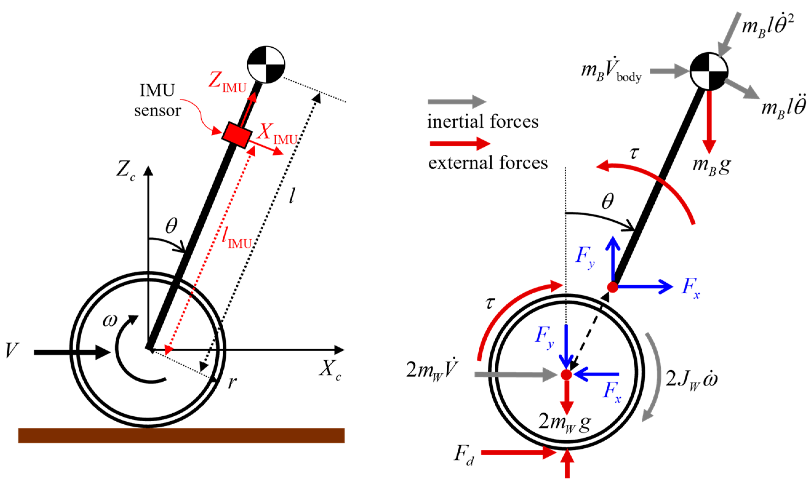
In the case where the pitch motion of the body is negligible, the chassis acceleration in the horizontal direction can be directly measured by a single one-axis accelerometer. As shown in
Figure 4, however, the IMU output in the longitudinal motion plane includes the tangential, centripetal, and gravitational components as well as the translational acceleration. Assuming that the IMU is installed at a distance
from the origin of the chassis frame, the acceleration components with regard to the sensor coordinates can be represented as:
where the chassis acceleration can be readily determined by proper transformations and using the real-time outputs of IMU.
The suggested slip indicator enables us to avoid the critical problem of estimating the true speed of the vehicle in applying the conventional slip ratio (4) and is free of the singular problem with an invariant denominator. If the value of (6) is close to zero, the wheel slip is very small, i.e., . If it is close to one, it says that a large wheel slip is happening because the wheel acceleration will be rapidly increased to the maximum by fast spinning of the wheel, i.e., .
3.3. Maximum Transmissble Torque Estimation
As mentioned in
Section 2, TWIP vehicles are more vulnerable to wheel slip compared with four-wheelers or three-wheelers without the risk of falling over. The root-cause of the problem comes from the fact that the two-degrees of freedom in longitudinal motion must be regulated by the single input corresponding to the torque sum of two parallel wheels due to the underactuated structure. In other words, the posture of the inverted pendulum body is indirectly controlled by the reaction torque according to the input-coupling phenomenon of the acrobot system [
21].
Here, we revisit the maximum transmissible torque estimation (MTTE) method. In estimating the maximum transmissible torque which can be wholly delivered to the wheel, the quarter vehicle model suggested in [
7] for a four-wheeled vehicle is not enough for a TWIP vehicle because it lacks the pitch motion of the chassis. In
Figure 4, the free body diagram regarding the longitudinal motion of TWIP is illustrated, where the vertical acceleration of the chassis frame is neglected for convenience. Then, the internal forces between the body and wheel shaft can be described as:
In addition, the dynamic equations of motion for the wheels can be simplified as:
where
is the translational driving force which can be varied according to the friction level of the ground and
is the average of the angular accelerations of both wheels. If we can obtain the real-time data with respect to the wheel torque and the angular acceleration of the wheels, the current driving force can be estimated as:
From (8) and (9), we can derive the ratio of the chassis acceleration to the wheel acceleration, which is correspondent to the relaxation factor defined in [
9].
Then, the maximum transmissible torque (MTT) to properly restrict the control input in real time can be determined as:
where the acceleration ratio
can be utilized as a design parameter.
Depending on the ground friction of the driving surface, the ratio can be chosen between zero and one to reconcile the driving performance for prompt velocity tracking and the anti-slip performance for the safety of the vehicle. For example, if , there is no arbitrary limit of control input without considering the wheel slip, and the motion control capacity is stressed. If the parameter approaches one, the MTT becomes smaller and more conservative control inputs will be drawn. Specifically, if , it indicates that the chassis acceleration of the vehicle is desired to be the same as the wheel acceleration without having any slippage.
3.4. A Modified MTTE Method with Slip Indicator
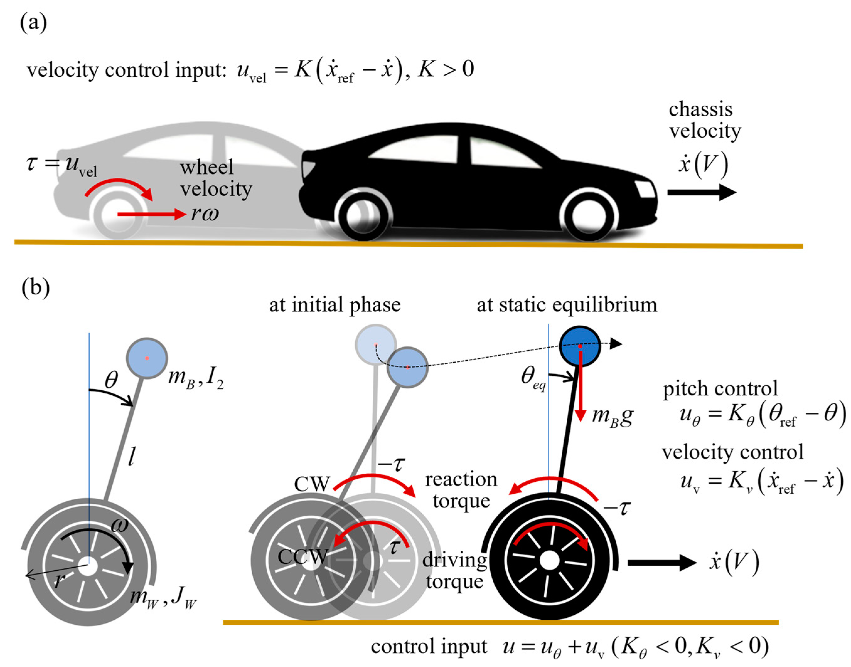
Following the conventional MTTE method, the wheel slip can be counteracted by restricting the control input within the estimated MTT according to (12), at all times while the vehicle is running. However, in the case that the uncertainties of plant parameters and feedback sensors are beyond a certain tolerance, the anti-slip control function will result in a great degradation of tracking performance in nonslip situations. If we consider that TWIP vehicles are expected to conduct agile motions by utilizing the extra degree of freedom of the inverted pendulum, it is not reasonable to apply the MTT even when the wheel slip is trivial. In that sense, the slip indicator in (6) is useful to switch the control input into the estimated MTT only when the indicator value is over a certain threshold. Considering the velocity control characteristic described in
Figure 1, it is very hard to stop the wheel slip of TWIP without falling over once it begins. Hence, it is critical to instantly detect the initiation of the wheel slip before it progresses. In this respect, the acceleration-based indicator is more effective than the conventional velocity-based slip ratio because the slipping phenomenon occurs mostly in the acceleration or deceleration phase to start, stop, and change the velocity.
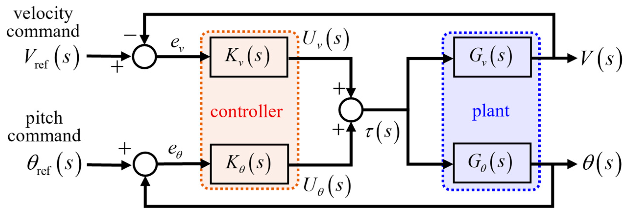
In applying the anti-slip control, the balancing performance must be prioritized for the safety of the vehicle rather than the wheel slip suppression itself, and the anti-slip function must not disturb the postural stability of the inverted pendulum body. Then, it is desirable to restrict only the velocity control input within the MTT but keep the pitch control input irrespective of the wheel slip occurrence. Consequently, the overall schematic of the proposed method is represented in
Figure 5. In other words, the anti-slip control loop is activated as soon as the slip indicator goes beyond the threshold, and the original velocity control mode is naturally recovered when the wheel slip is weakened with smaller indicator values. For the slip indicator, it is respectively calculated for each wheel, and the anti-slip control is simultaneously applied to both wheels if one of them becomes larger than the threshold. In real implementation, the actual wheel torque to estimate the current driving force can be estimated in real time by multiplying the motor current, torque constant, gear ratio, and gear efficiency, and the angular acceleration of each wheel can be reliably determined by the numerical differentiation of encoder outputs.
The proposed anti-slip control loop contains two tuning parameters. First, the switching of the velocity control input to the MTT value is determined by the threshold of the slip indicator (6). The threshold value represents how much slippage is allowed in the wheels. Considering that the speed of TWIP vehicles is relatively lower than commercial four-wheelers and the stability margin of the pitch control loop is very small, it is reasonable to let the value be as small as possible on slippery surfaces. In real situations where the driving environment is furnished, the threshold can be empirically determined. Second, the closer the acceleration ratio (11) to one, the MTT value of the torque limiter becomes smaller. If the safety associated with not falling over is the top priority, it is recommended to fix the ratio as . However, it may greatly limit the maneuvering capability of a TWIP vehicle in non-slippery surfaces due to the restricted control torque.
4. Numerical Experiment
When a TWIP robotic vehicle accelerates to start or decelerates to stop on low frictional surfaces, the driving torque is enough to trigger a wheel slip. In addition, if the TWIP robot falls from a low step, the driving wheels lose traction and spin freely for a moment as the wheels are off the surface of the step. For these driving conditions, comparative simulations are conducted by applying three different types of controllers as represented in
Figure 6. In Case 1, it consists of the baseline controllers, PD for pitch control and PI for velocity control, respectively. In Cases 2 and 3, the conventional MTTE and the proposed method are applied, respectively, in company with the baseline controller.
The TWIP robot system model with the specs in
Table 2 and the virtual driving surfaces have been established through the Matlab Simscape multibody toolbox [
22]. It provides elaborate dynamic modeling tools for links, joints, actuators, and sensors and enables endowing attributes to surfaces and contact points. For the anti-slip control parameters, the threshold of slip indicator has been chosen as
and the acceleration ratio for MTTE as
. For the baseline controller for velocity tracking and pose stabilization, negative feedback gains as
are assigned. For the driving surface, the static and dynamic friction coefficients of the nonslip section are
,
assuming a normal indoor floor, and those of the slippery section are
,
assuming an icy road, respectively. The video clips for the simulation results in
Figure 7,
Figure 8,
Figure 9,
Figure 10,
Figure 11,
Figure 12,
Figure 13 and
Figure 14 can be found at
https://youtu.be/msGiHrY8_TQ (accessed on 22 April 2023).
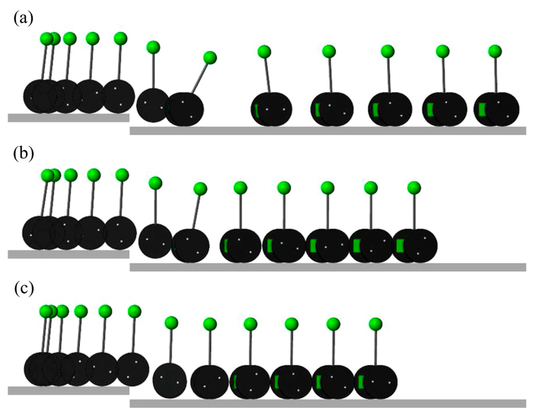
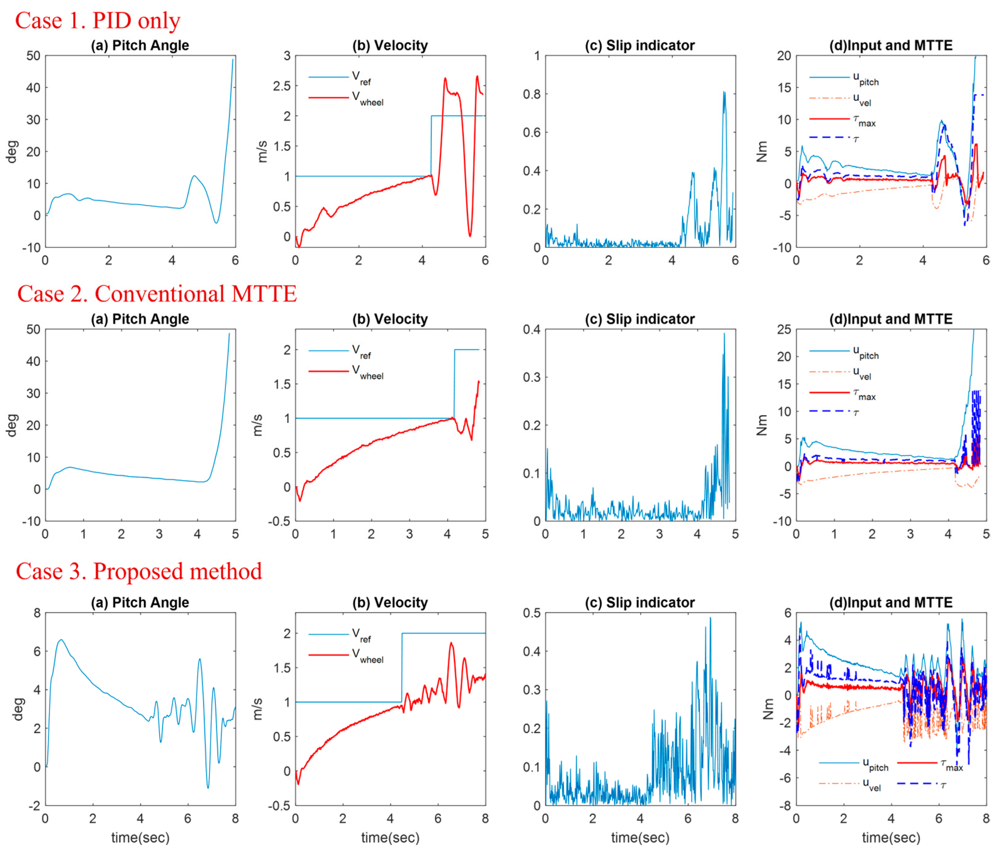
4.1. Acceleration Phase to Start on Low-Frictional Surface
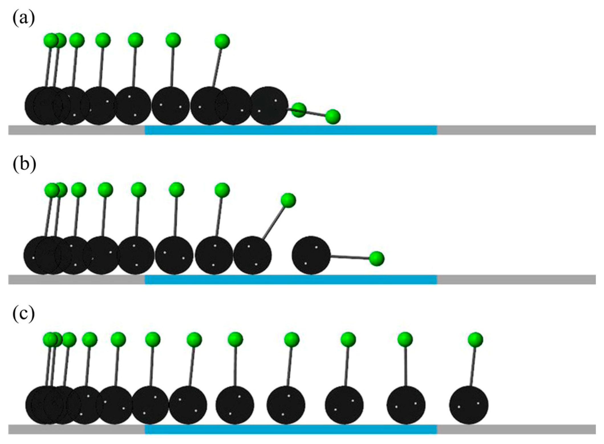
In
Figure 7 and
Figure 8, the TWIP robot starts to develop the initial reference velocity of 1 m/s and speeds up to 2 m/s at 3 s, which is in common for all three cases. The inverted pendulum naturally leans forward in accordance with the clockwise reaction torque activated as the driving wheels accelerate to speed up. In Case 1, the robot experiences a severe wheel slip around 3 s on the slippery section as soon as the control input is increased to track the target speed. Surely, the residual of the PID control input over the MTT makes the wheels lose traction and the robot eventually falls over in the forward direction. In Case 2, the conventional MTTE technique enables it to stop the slipping of wheels according to the input torque limitation, but the inverted pendulum body loses its pitch balance because even the pitch control input is limited together. In contrast, with Case 3, the proposed method makes the robot pass through the slippery section safely, where a little oscillatory pitch motion is due to the on-off operation of the slip indicator. As shown in
Figure 8c, the acceleration-based slip indicator is enough to detect the occurrence of the wheel slip.
4.2. Deceleration Phase to Stop on Low-Frictional Surface
In
Figure 9 and
Figure 10, the TWIP robot commonly enters the slippery section with the speed of 1 m/s, and the zero-velocity reference command is assigned at 3 s to make the robot stop. In Case 1, the pendulum body naturally leans backward by the counterclockwise reaction torque occurring when the wheels are decelerated, and the pendulum body does not recover its pitch balance because the PID control input cannot be wholly transferred to the contact surface on the slippery section. In Case 2, the wheel slip is considerably reduced when compared with Case 1 as the slip indicator value represents. However, the restriction of the entire control input leads to failure in the posture control. In Case 3, the MTT limiter to the velocity control instantly operates as the slip indicator exceeds the threshold, and the pitch control input is sufficiently converted into the traction force on the wheels. As a result, the robot gradually comes to a stop in the slippery section while keeping its upright posture.
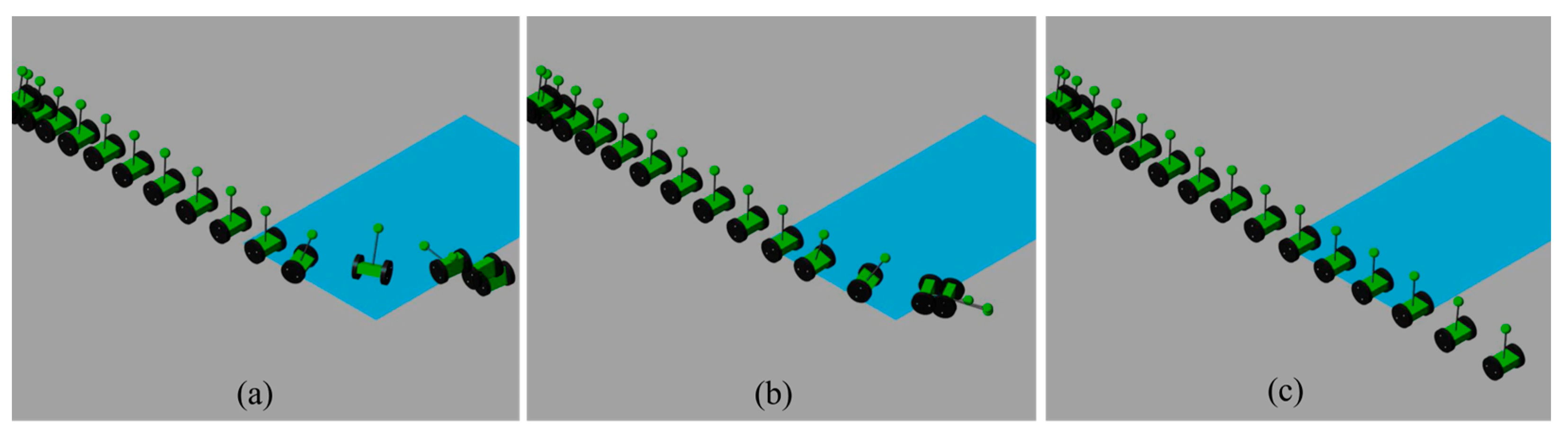
4.3. Rolling down from a Step
In
Figure 11 and
Figure 12, the TWIP robot rolls down to the floor from a 15 cm high step. Then, the robot undergoes a short free fall phase when the driving wheels spin freely without ground friction. Depending on how the robot counteracts the tractionless moment, the behavior of the inverted pendulum body is determined after the wheels contact the normal surface again. In Case 1, the wheel speed is rapidly increased as soon as the traction vanishes as the sharp increase of the slip indicator is shown at about 2.5 s. In the airborne state during the free fall, the velocity control input without limitation will accelerate the spinning, which results in a large pitch down or even pitch over just after regaining the wheel traction on the surface. In Case 2, the fluctuation of pitch motion has been considerably reduced because the MTTE technique reduces the spinning of wheels before making contact with the surface. In Case 3, we have the smallest variation of the pitch angle with the lowest possibility of falling over. It indicates that the proposed method enhances the reliability of TWIP vehicles on uncertain surfaces.
4.4. Solo Wheel Slippage under Yaw Rate Control
We have assumed the longitudinal motion of a TWIP in the anti-slip control formulation. However, it can be readily applied to three-dimensional cases including yaw motion. In
Figure 13 and
Figure 14, only the left wheel of TWIP meets the slippery surface while the vehicle is accelerated. In Case 1, the left wheel spins fast as soon as it loses traction. Although the yaw rate control is activated, a heavy yawing motion arises due to the unbalanced ground friction, and the vehicle eventually falls over. In Case 2, the vehicle has a less yaw motion owing to the restricted torque input by the MTTE algorithm, but it fails to keep the postural stability. In Case 3, the vehicle safely escapes from the low-frictional surface and the yaw motion is successfully regulated. As shown in
Figure 14d, only the left wheel is over the threshold of the slip indicator, but the MTT according to (12) is equally distributed to both wheels. As a result, the velocities of the left and right wheel denote similar values in
Figure 14b.
5. Robot Experiment
The hardware control system for the experiment is shown in
Figure 6, where it consists of right and left wheel motors with built-in encoders, an IMU sensor, and a control processor (mini-PC with Windows 10 OS). The control software integration was performed using Visual Studio 2017. The system parameters of the TWIP vehicle are the same as the simulation model in
Table 2. Additionally, the anti-slip control parameters were set up the same as the numerical experiments in the former section, i.e., threshold of the slip indicator
, acceleration ratio
. The feedback gains of the baseline controller are commonly given as
for the three cases in the following comparative experiments. That is, all of them have negative signs. The difference of scale in the magnitude of gains from the simulation cases comes from the fact that the electrical part of the real system is not included in the simulation model. On the other hand, to furnish a slippery surface which has a low frictional coefficient on an indoor floor, we used Teflon grease spread on an acrylic mat as denoted in
Figure 15. The grease was reapplied in each test run to make almost the same slippery condition.
Prior to the comparative experiments, it is necessary to note that the wheel slip on a slippery road occurs only if the control torque exceeding the friction level between the wheels and surface is applied. When a TWIP vehicle is travelling at a steady state with a constant speed and pitch angle, a severe wheel slip will not happen because it needs only a small driving torque comparable to the rolling resistance to maintain the current speed and pose. The TWIP vehicles will generate a sufficiently large wheel torque to trigger the wheel slip when the speed is going to change, or the pitch angle must recover its equilibrium point. The video clips related to the experimental results in
Figure 15,
Figure 16,
Figure 17 and
Figure 18 can be accessed at
https://youtu.be/msGiHrY8_TQ (accessed on 22 April 2023).
5.1. Passing through Slippery Section in Acceleration Phase
In
Figure 15 and
Figure 16, the TWIP robot in the acceleration phase enters the slippery section at around 4 s as the slip indicator represents in
Figure 14c. In Case 1, the nominal PID control is applied without an anti-slip function. When the velocity reference is increased to 2 m/s soon after 4 s, it makes the body tilt forward and then the pith control input is generated to recover its upright posture. As shown in
Figure 16a, the robot restores its pitch balance for a moment around 5 s despite the wheel slip by the pitch control action, but the robot eventually topples over as the excessive control input over the MTT is continuously applied. For the safety of the vehicle, the battery power is shut off when the pitch angle is over 50 deg. In Case 2, the robot tilts forward in the same way. However, it fails to restore the pitch balance unlike Case 1 since the entire control input is limited within the estimated MTT irrespective of the wheel slip occurrence. In contrast, in Case 3, employing the proposed method, the robot successfully escapes from the slippery section while keeping a balancing pose, where the fluctuating pitch motions are due to the switching-type torque limiter. As shown in
Figure 16b, the velocity tracking performance is very poor even in Case 3, because the balancing performance of the inverted pendulum is prioritized in the anti-slip control.
5.2. Passing through Slippery Section in Deceleration Phase
In
Figure 17 and
Figure 18, the zero-velocity reference is assigned to the robot as a stop command soon after 4 s, when the robot enters the slippery low frictional surface. In Case 1, the robot tilts backward in accordance with the deceleration phase and it is followed by a rebalancing motion. In the end, it falls over while losing the wheel traction because the unlimited control torque is continuously applied. In Case 2, it does not recover the equilibrium state of the pitch angle and finally loses its pitch balance in the same logic as the acceleration phase. In Case 3, as we have expected, the proposed method helps the robot to keep its postural stability in the slippery section by adjusting the velocity control input properly with the slip indicator-based switching function and fully allowing the pitch control input.


