
Active Fault Diagnosis and Control of a Morphing Multirotor Subject to a Stuck Arm †


Abstract
:1. Introduction
2. Mathematical Model
- is the position of (decomposed in );
- is the angular velocity of relative to (decomposed in );
- m is the total system mass, g is the gravitational acceleration, and and are the linear and angular friction coefficients;
- and are the gravitational and the (unknown) wind forces (decomposed in );
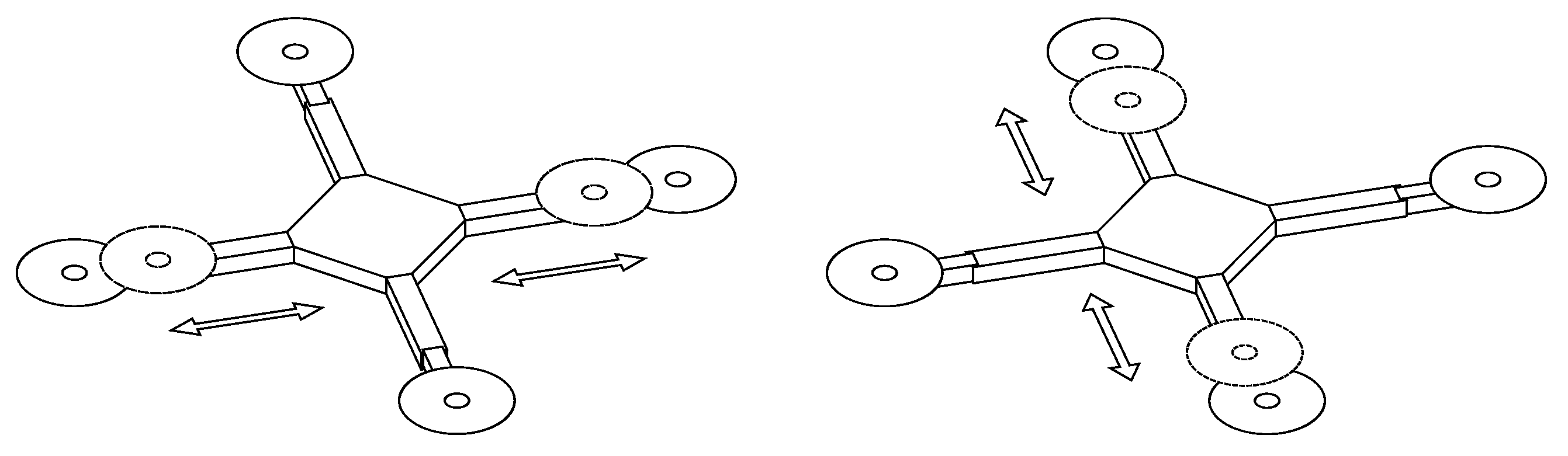
- is the vector containing the arm lengths of each motor (see Figure 1);
- is the arm-dependent center of mass (decomposed in );
- is the arm-dependent inertia matrix of the overall system, relative to the center of mass;
- and are the arm-dependent thrust and torque due to the actuators (both decomposed in );
- is the vector composed by the roll (), pitch (), and yaw angles, which let us express the rotation matrix from to , denoted as , aswhere and are considered for the sake of brevity;
- is the kinematic coordinate transformation related to the adopted roll–pitch–yaw rotation.
- no torques due to the wind are considered;
- additional forces and torques due to blade flapping are of a smaller magnitude and neglected;
- the friction force is assumed to be linear, with proportional coefficients , .
2.1. Total Mass
2.2. Center of Mass
2.3. Inertia Matrix
2.4. Actuation Force and Moment
2.5. Inputs and Faults
3. Symmetries and Sensitivity
- The arms are counter-clockwise numbered and equally distributed on the so-called “x” configuration, leading to the angles
- The overall geometry of each arm is identical to the others. In particular, the geometry constraints of each fixed arm and telescopic arm lead towhile the geometry constraints of each motor and rotor lead to
- For each arm, the mass of each component is equal to the corresponding component of the other arms, which leads to
- Motors 1 and 3 are counter-clockwise, while 2 and 4 are clockwise, henceSeveral implications follow.
- The total mass of the system is
- Since and , for each vector we have
4. Fault Detection, Isolation, and Identification
4.1. Fault Detection
- 1.
- whenever no fault occurs, exhibits convergent dynamics;
- 2.
- whenever a fault occurs, at least one component of does not exhibit convergent dynamics.
4.2. Fault Isolation
- 1.
- whenever occurs, exhibits convergent dynamics for ;
- 2.
- whenever occurs, for , does not exhibit convergent dynamics, while exhibits convergent dynamics for each .
- 1.
- If , then and exhibits asymptotically stable dynamics.
- 2.
- If , then exhibits asymptotically stable dynamics, while is achieved in finite time.
- 3.
- If , then exhibits asymptotically stable dynamics, while is achieved in finite time.
- 4.
- If , then exhibits asymptotically stable dynamics, while is achieved in finite time.
- 5.
- If , then exhibits asymptotically stable dynamics, while is achieved in finite time.
4.3. Active Fault Isolation and Identification
- 1.
- If and are strictly increasing, then becomes strictly decreasing after a finite time.
- 2.
- If and are strictly decreasing, then becomes strictly decreasing after a finite time.
- : no fault is detected or isolated. The output is ;
- : the i-th arm has been isolated (respectively, for some ) and the corresponding stuck fault is estimated as . Denoting the stuck arm with i, the output is for and ;
- and : the fault class for the first or for the second has been isolated (as described by the second “+” and “−” signs, respectively). Denoting the switching time with , the supervisor overrides and with the increasing commands (as described by the first “+” sign in both system states)
- and : the fault class (for the first) or (for the second) has been isolated. Denoting the switching time with , the supervisor overrides and with the decreasing commands
- and : the fault class (for the first) or (for the second) has been isolated. Denoting with the switching time, the supervisor overrides and with the increasing commands
- and : the fault class (for the first) or (for the second) has been isolated. Denoting the switching time as , the supervisor overrides and with the decreasing commands
- : no fault class is currently isolated from the ;
- : the corresponding fault class has been isolated from the ;
- and : is achieved for the former, while for the latter;
- and : is achieved for the former, while for the latter.
5. Fault-Tolerant DOBC Control
6. Numerical Simulations
- Frequencies. The simulation is carried out for a total of 30 s. According to the double-loop structure, faster inner loop dynamics are achieved by both control parameters and different sample times. This solution takes into consideration computational limitations on a future implementation. In particular, the inner loop is simulated at 1 kHz, while the outer loop runs at 10 Hz. A zero order hold is applied for and between consecutive samples.
- Plant parameters. The frame and fixed arms are those of a DJI Flamewheel 450, the telescopic arms are of the same size and mass as the fixed ones, and the electric motors are the T-Motor AirGear 350. Table 3 summarizes the geometric dimensions and the dynamic parameters.
- Sensors and Inertial Measurement Unit (IMU). The commonly adopted MPU-9250 IMU [28] is taken into consideration. Additive white Gaussian noise is applied to accelerations and gyroscopes, with standard deviation and , respectively. Finally, due to Kalman filtering, a smaller noise is assumed for simplicity on attitude, linear velocity, and linear position (i.e., , , , respectively).
- Input saturation. A saturation is considered for each actual lift force. The total mass of the system is 1.448 kg, resulting in a thrust-to-weight ratio equal to .
- Control parameters. All the control parameters have been heuristically set. The parameters for both the control law and the observer are summarized in Table 3.
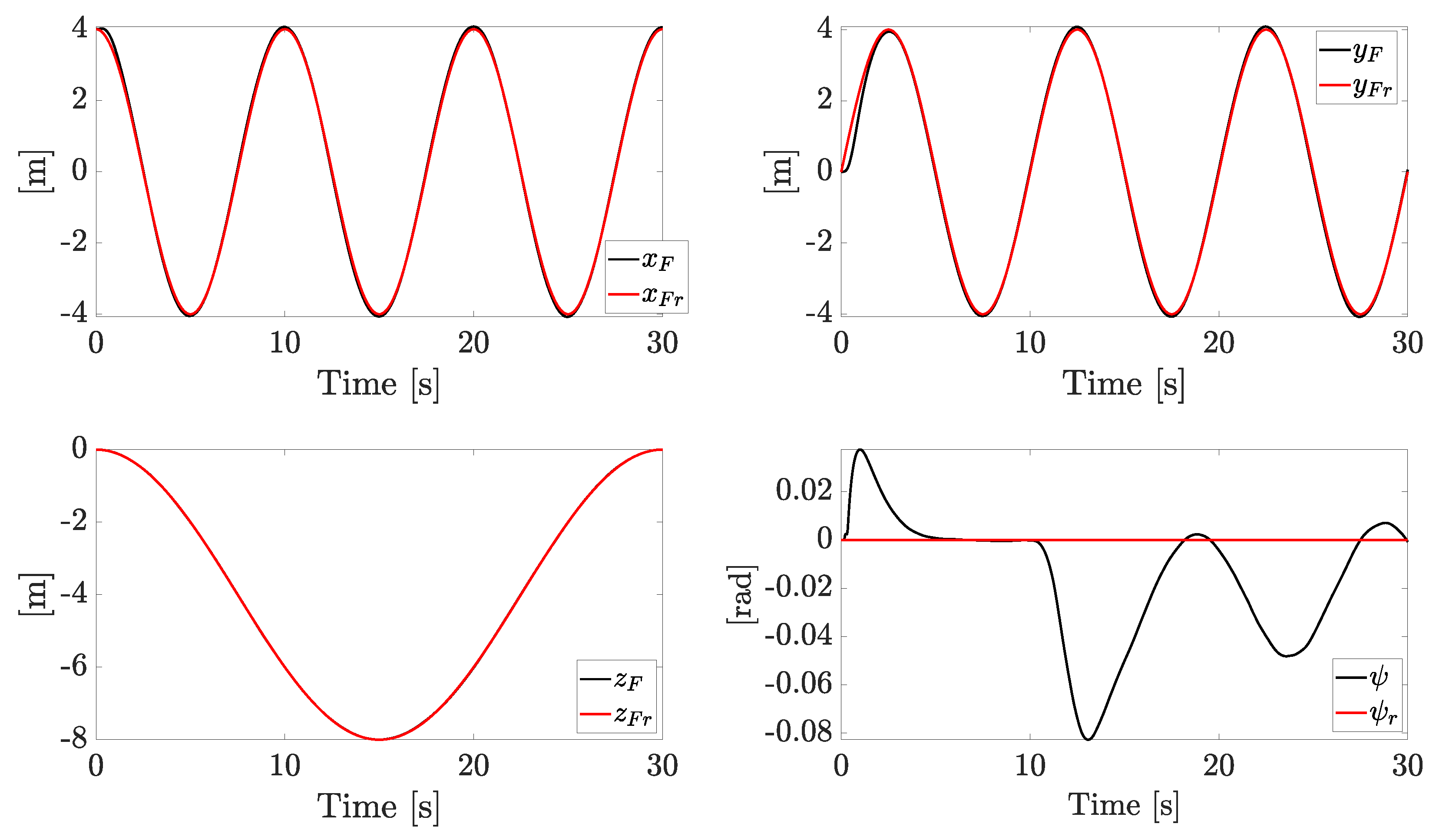
6.1. Scenario 1
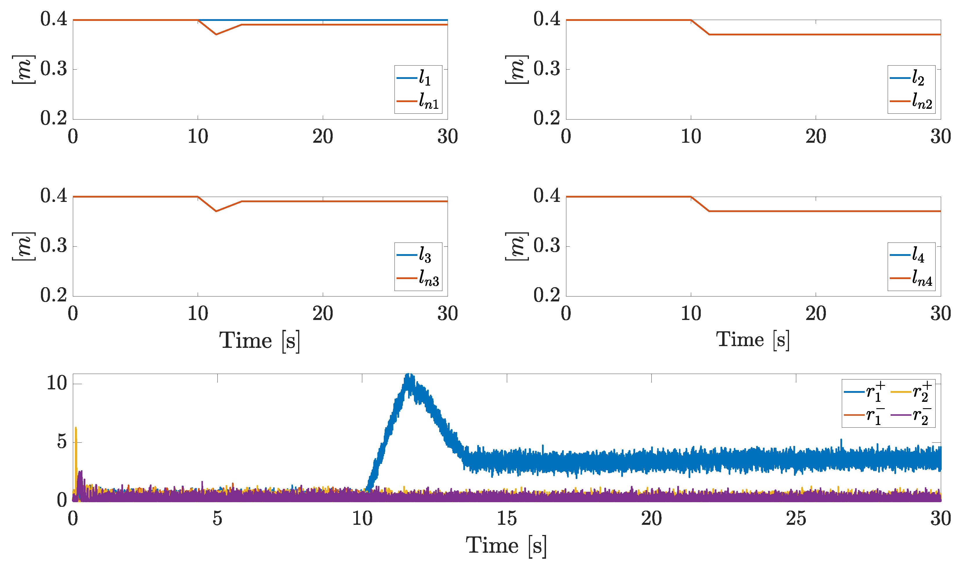
6.2. Scenario 2
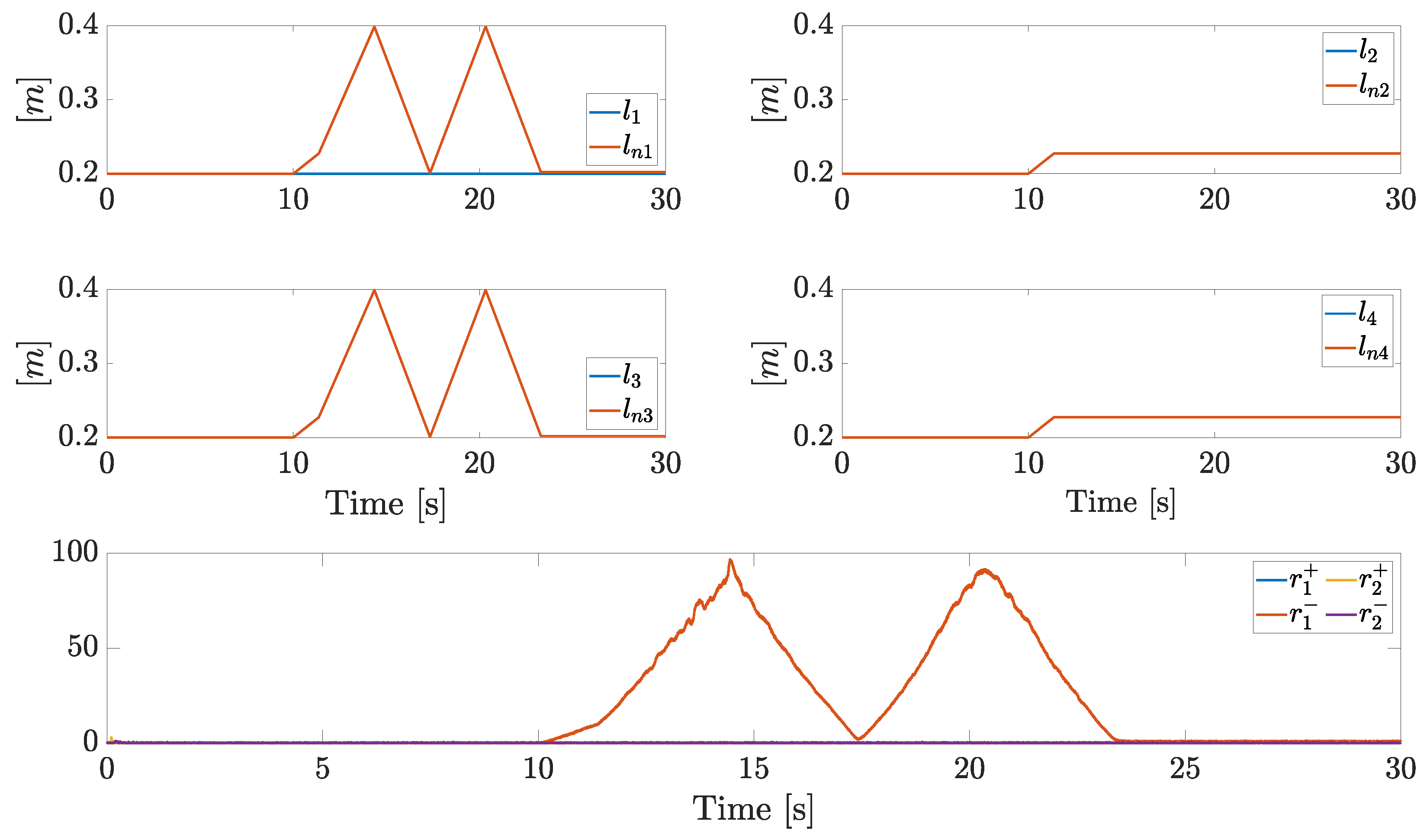
6.3. Scenario 3
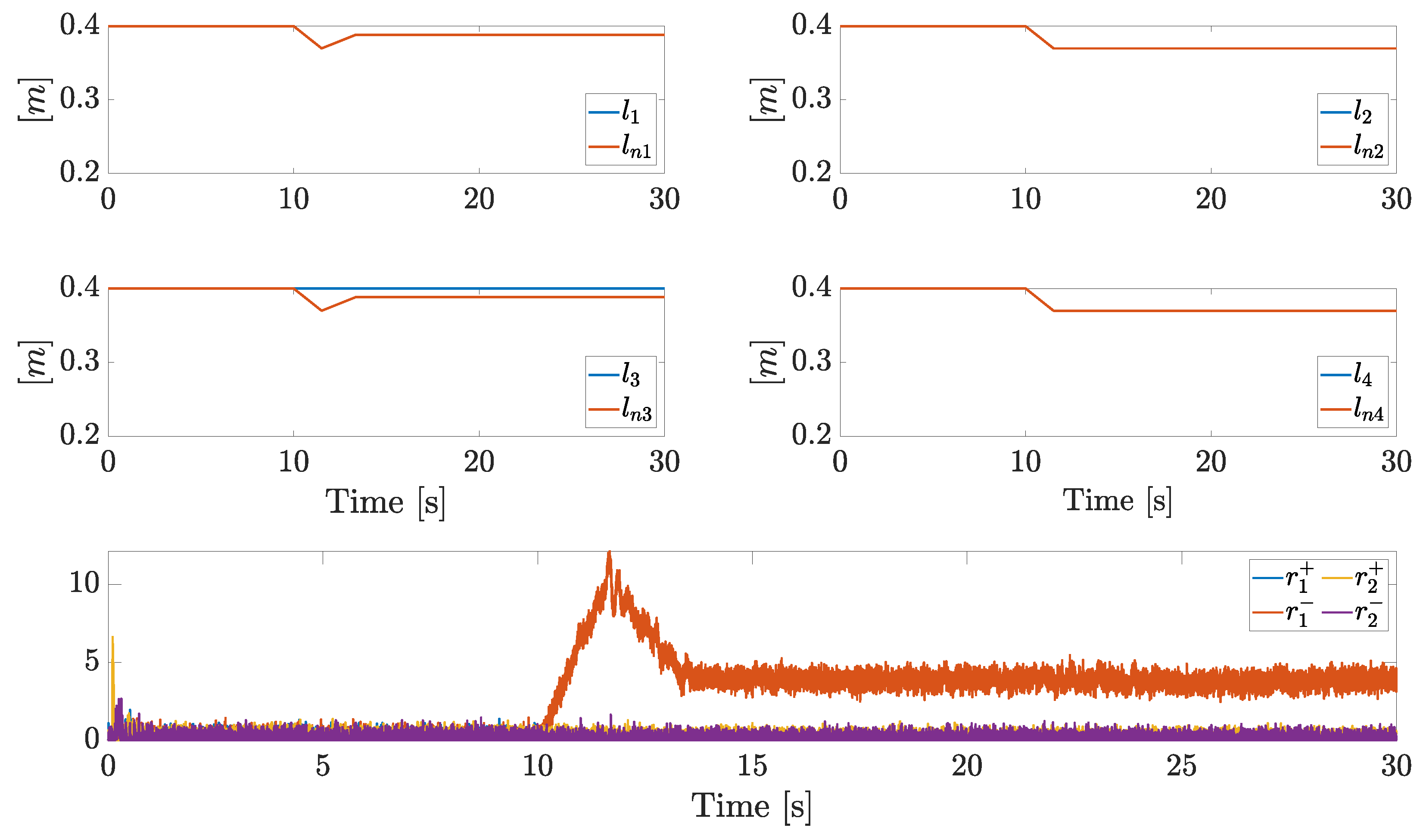
6.4. Scenario 4
7. Conclusions
Author Contributions
Funding
Institutional Review Board Statement
Informed Consent Statement
Data Availability Statement
Conflicts of Interest
Abbreviations
| DO | Disturbance Observer |
| DOBC | Disturbance Observer-Based Control |
| FDD | Fault Detection and Diagnosis |
| FD | Fault Detection |
| FDI | Fault Detection and Isolation |
| FI | Fault Isolation |
| FId | Fault Identification |
| FTC | Fault Tolerant Control |
| NDO | Nonlinear Disturbance Observer |
| UAV | Unmanned Aerial Vehicle |
Appendix A
Appendix A.1. Proof of Remark 9
Appendix A.2. Proof of Remark 10
References
- Pütsep, K.; Rassõlkin, A. Methodology for Flight Controllers for Nano, Micro and Mini Drones Classification. In Proceedings of the 2021 International Conference on Engineering and Emerging Technologies (ICEET), Istanbul, Turkey, 27–28 October 2021; pp. 1–8. [Google Scholar] [CrossRef]
- Longhi, M.; Taylor, Z.; Popović, M.; Nieto, J.; Marrocco, G.; Siegwart, R. RFID-Based Localization for Greenhouses Monitoring Using MAVs. In Proceedings of the 2018 IEEE-APS Topical Conference on Antennas and Propagation in Wireless Communications (APWC), Columbia, SC, USA, 10–14 September 2018; pp. 905–908. [Google Scholar] [CrossRef]
- Cutler, M.; How, J.P. Analysis and control of a variable-pitch quadrotor for agile flight. J. Dyn. Syst. Meas. Control 2015, 137, 101002. [Google Scholar] [CrossRef]
- Niemiec, R.; Gandhi, F.; Lopez, M.; Tischler, M. System identification and handling qualities predictions of an eVTOL urban air mobility aircraft using modern flight control methods. In Proceedings of the Vertical Flight Society 76th Annual Forum, Virtual, 5–8 October 2020. [Google Scholar]
- Wang, Z.; Groß, R.; Zhao, S. Controllability analysis and controller design for variable-pitch propeller quadcopters with one propeller failure. Adv. Control. Appl. Eng. Ind. Syst. 2020, 2, e29. [Google Scholar] [CrossRef]
- Baldini, A.; Felicetti, R.; Freddi, A.; Longhi, S.; Monteriù, A. Actuator fault tolerant control of variable pitch quadrotor vehicles. IFAC-PapersOnLine 2020, 53, 4095–4102. [Google Scholar] [CrossRef]
- Tuna, T.; Ovur, S.E.; Gokbel, E.; Kumbasar, T. Design and development of FOLLY: A self-foldable and self-deployable quadcopter. Aerosp. Sci. Technol. 2020, 100, 105807. [Google Scholar] [CrossRef]
- Peraza-Hernandez, E.A.; Hartl, D.J.; Malak, R.J., Jr.; Lagoudas, D.C. Origami-inspired active structures: A synthesis and review. Smart Mater. Struct. 2014, 23, 094001. [Google Scholar] [CrossRef]
- Mintchev, S.; Floreano, D. A pocket sized foldable quadcopter for situational awareness and reconnaissance. In Proceedings of the 2016 IEEE International Symposium on Safety, Security, and Rescue Robotics (SSRR), Lausanne, Switzerland, 23–27 October 2016; pp. 396–401. [Google Scholar]
- Shu, J.; Chirarattananon, P. A quadrotor with an origami-inspired protective mechanism. IEEE Robot. Autom. Lett. 2019, 4, 3820–3827. [Google Scholar] [CrossRef]
- Avant, T.; Lee, U.; Katona, B.; Morgansen, K. Dynamics, hover configurations, and rotor failure restabilization of a morphing quadrotor. In Proceedings of the 2018 IEEE American Control Conference (ACC), Milwaukee, WI, USA, 27–28 June 2018; pp. 4855–4862. [Google Scholar]
- Brischetto, S.; Ciano, A.; Ferro, C.G. A multipurpose modular drone with adjustable arms produced via the FDM additive manufacturing process. Curved Layer. Struct. 2016, 3, 202–213. [Google Scholar] [CrossRef]
- Falanga, D.; Kleber, K.; Mintchev, S.; Floreano, D.; Scaramuzza, D. The foldable drone: A morphing quadrotor that can squeeze and fly. IEEE Robot. Autom. Lett. 2018, 4, 209–216. [Google Scholar] [CrossRef]
- Desbiez, A.; Expert, F.; Boyron, M.; Diperi, J.; Viollet, S.; Ruffier, F. X-Morf: A crash-separable quadrotor that morfs its X-geometry in flight. In Proceedings of the 2017 Workshop on Research, Education and Development of Unmanned Aerial Systems (RED-UAS), Linkoping, Sweden, 3–5 October 2017; pp. 222–227. [Google Scholar]
- Derrouaoui, S.; Guiatni, M.; Bouzid, Y.; Dib, I.; Moudjari, N. Dynamic modeling of a transformable quadrotor. In Proceedings of the 2020 International Conference on Unmanned Aircraft Systems (ICUAS), Athens, Greece, 1–4 September 2020; pp. 1714–1719. [Google Scholar]
- Zhao, M.; Kawasaki, K.; Chen, X.; Noda, S.; Okada, K.; Inaba, M. Whole-body aerial manipulation by transformable multirotor with two-dimensional multilinks. In Proceedings of the 2017 IEEE International Conference on Robotics and Automation (ICRA), Singapore, 29 May–3 June 2017; pp. 5175–5182. [Google Scholar]
- Pose, C.; Giribet, J. Multirotor fault tolerance based on center-of-mass shifting in case of rotor failure. In Proceedings of the 2021 International Conference on Unmanned Aircraft Systems (ICUAS), Athens, Greece, 15–18 June 2021; pp. 38–46. [Google Scholar]
- Kumar, R.; Deshpande, A.M.; Wells, J.Z.; Kumar, M. Flight control of sliding arm quadcopter with dynamic structural parameters. In Proceedings of the 2020 IEEE/RSJ International Conference on Intelligent Robots and Systems (IROS), Las Vegas, NV, USA, 24 October 2020–24 January 2021; pp. 1358–1363. [Google Scholar]
- Xu, C.; Yang, Z.; Zhang, Z.; Xu, H.; Wu, J.; Zhou, D.; Liao, L.; Zhang, Q. Design and Control of a Deformable Trees-Pruning Aerial Robot. Complexity 2020, 2020, 6627339. [Google Scholar] [CrossRef]
- Tomić, T.; Ott, C.; Haddadin, S. External wrench estimation, collision detection, and reflex reaction for flying robots. IEEE Trans. Robot. 2017, 33, 1467–1482. [Google Scholar] [CrossRef]
- Li, S.; Yang, J.; Chen, W.; Chen, X. Disturbance Observer-Based Control: Methods and Applications; CRC Press: Boca Raton, FL, USA; Taylor & Francis Group: Abingdon, UK, 2017. [Google Scholar]
- De Persis, C.; Isidori, A. A geometric approach to nonlinear fault detection and isolation. IEEE Trans. Autom. Control 2001, 46, 853–865. [Google Scholar] [CrossRef]
- Isermann, R. Fault-Diagnosis Systems: An Introduction from Fault Detection to Fault Tolerance; Springer: Berlin/Heidelberg, Germany, 2005. [Google Scholar]
- Chen, J.; Patton, R. Robust Model-Based Fault Diagnosis for Dynamic Systems; Springer: New York, NY, USA, 2012. [Google Scholar]
- Baldini, A.; Felicetti, R.; Freddi, A.; Longhi, S.; Monteriù, A. Modeling and Control of a Telescopic Quadrotor Using Disturbance Observer Based Control. In Proceedings of the 2022 30th Mediterranean Conference on Control and Automation (MED), Athens, Greece, 28 June–1 July 2022; pp. 396–402. [Google Scholar] [CrossRef]
- Fossen, T. Guidance and Control of Ocean Vehicles; Wiley: Hoboken, NJ, USA, 1994. [Google Scholar]
- Michieletto, G.; Ryll, M.; Franchi, A. Fundamental actuation properties of multirotors: Force–moment decoupling and fail–safe robustness. IEEE Trans. Robot. 2018, 34, 702–715. [Google Scholar] [CrossRef]
- TDK InvenSense. MPU-9250, Nine-Axis (Gyro + Accelerometer + Compass) MEMS MotionTracking™ Device. 2016. Available online: https://invensense.tdk.com/download-pdf/mpu-9250-datasheet/ (accessed on 24 March 2023).
- Becker, M.; Sampaio, R.C.B.; Bouabdallah, S.; Perrot, V.d.; Siegwart, R. In-flight collision avoidance controller based only on OS4 embedded sensors. J. Braz. Soc. Mech. Sci. Eng. 2012, 34, 294–307. [Google Scholar] [CrossRef]


| 0 | 0 | ||
| 0 | 0 |
| 0 | 0 | 0 | |||
| 0 | 0 | 0 | |||
| 0 | 0 | 0 | 0 | ||
| 0 | 0 | 0 | 0 | ||
| 0 | 0 | 0 | 0 | ||
| 0 | 0 | 0 | 0 |
| Parameters | Variables | Value | Unit |
|---|---|---|---|
| Frame width and length | (m) | ||
| Frame height | (m) | ||
| Fixed and telescopic arm widths | (, ) | (m) | |
| Fixed and telescopic arm lengths | (, ) | (m) | |
| Motor radius | () | (m) | |
| Rotor radius | () | (m) | |
| Fixed and telescopic arms heights | (, ) | (m) | |
| Motor heights | () | (m) | |
| Rotor heights | () | (m) | |
| Minimum arm length | (m) | ||
| Maximum arm length | (m) | ||
| Frame mass | (kg) | ||
| Fixed and telescopic arm masses | (, ) | (kg) | |
| Motor masses | () | (kg) | |
| Rotor masses | () | (kg) | |
| Total system mass | m | (kg) | |
| Gravitational acceleration | g | (m/s) | |
| Linear friction coefficient | (N·s/m) | ||
| Angular friction coefficient | (N·s·m) | ||
| Lift coefficient | (N·s) | ||
| Drag coefficient | (N· m) | ||
| Inner loop frequency | (Hz) | ||
| Outer loop frequency | 10 | (Hz) | |
| Control input lower saturation | 0 | (N) | |
| Control input upper saturation | 9 | (N) | |
| and closed loop poles | |||
| closed loop poles | |||
| and closed loop poles | |||
| closed loop poles | |||
| Residual generator gains | 10 | ||
| Observer gain | H | ||
| Threshold 1 | 10 | ||
| Threshold 2 | 3 | ||
| Minimum time for each state | 1 | (s) |
Disclaimer/Publisher’s Note: The statements, opinions and data contained in all publications are solely those of the individual author(s) and contributor(s) and not of MDPI and/or the editor(s). MDPI and/or the editor(s) disclaim responsibility for any injury to people or property resulting from any ideas, methods, instructions or products referred to in the content. |
© 2023 by the authors. Licensee MDPI, Basel, Switzerland. This article is an open access article distributed under the terms and conditions of the Creative Commons Attribution (CC BY) license (https://creativecommons.org/licenses/by/4.0/).
Share and Cite
Baldini, A.; Felicetti, R.; Freddi, A.; Monteriù, A. Active Fault Diagnosis and Control of a Morphing Multirotor Subject to a Stuck Arm. Machines 2023, 11, 511. https://doi.org/10.3390/machines11050511
Baldini A, Felicetti R, Freddi A, Monteriù A. Active Fault Diagnosis and Control of a Morphing Multirotor Subject to a Stuck Arm. Machines. 2023; 11(5):511. https://doi.org/10.3390/machines11050511
Chicago/Turabian StyleBaldini, Alessandro, Riccardo Felicetti, Alessandro Freddi, and Andrea Monteriù. 2023. "Active Fault Diagnosis and Control of a Morphing Multirotor Subject to a Stuck Arm" Machines 11, no. 5: 511. https://doi.org/10.3390/machines11050511