An Indirect Procedure for Real-Time Monitoring the Neutral Conductor Deterioration in Three-Phase Distribution Networks

Abstract

An indirect procedure for real-time monitoring the neutral conductor condition in three-phase distribution networks, based on watching over the growth of a novel parameter (∆τ), has been described in this paper. The parameter ∆τ has been defined as the relationship between the neutral-displacement power and Buchholz’s apparent power measured at the fundamental frequency in the loads of the distribution networks for any condition of the neutral conductor and in its nominal conditions. The effectiveness of this procedure has been compared with other traditional indirect procedures, such as the surveillance of the RMS values of the line-to-neutral load voltages or their zero-sequence component. The practical application on a real distribution network reveals that the growth of the parameter ∆τ in the early stages of the breaking process of the neutral conductor follows a straight line whose equation is known for each length and section of that conductor, regardless of the loads and the voltage regulation of the transformer of the distribution network. This characteristic of the ∆τ parameter shows that the proposed procedure is suitable for monitoring neutral conductor deterioration and can be used for preventive maintenance of distribution networks.

1. Introduction

The state of the neutral conductor is of special interest for the proper operation of Low Voltage (LV) three-phase distribution networks. The presence of unbalanced and non-linear loads in the distribution networks causes high currents to flow through the neutral conductor as well as voltage drops, which increase the unbalanced voltages in the phases of the wye-configured loads [1,2,3] due to the well-known neutral-displacement phenomenon [4,5,6]. This phenomenon can reduce the useful life and the proper operation of the loads; thus, the equitable distribution of the loads between the phases of the distribution network is required [7] to avoid these undesirable effects of load imbalances. However, this problem is currently getting worse with the introduction of single-phase loads in three-phase networks, such as electric vehicle charging points [8,9].

The increase in the neutral conductor impedance due to its deterioration or accidental breakage usually has much more serious effects on the proper operation of distribution networks than load imbalances. The breakage of the neutral conductor intensifies the effects of the neutral-displacement phenomenon, causing over-voltages in the unbalanced loads [10,11,12,13].

In order to prevent the undesirable effects of deterioration or accidental breakage of the neutral conductor, indirect procedures have traditionally been used based on monitoring the RMS (Root Mean Square) values of the line-to-neutral load voltages or their zero-sequence component, complemented by the use of relays of maximum voltage or equivalent electronic devices [14,15,16]. These procedures are founded in the increase suffered by the neutral-displacement voltage ($V_{N{N}^{\prime }}$, Figure 1), due to the increase in the neutral conductor impedance during the breaking process. These voltages are of zero-sequence and are added to the line-to-neutral load voltages, increasing the RMS values in some load phases (over-voltages) and decreasing the RMS values in others (under-voltages). However, traditional procedures have the following drawbacks, which make them less effective in our opinion:

• The phases in which over-voltages and under-voltages occur often change depending on the loads.
• For a given line, the values of over-voltages and under-voltages, as well as the neutral-displacement voltages, caused by the deterioration of the neutral conductor, depend on the load imbalances and the values of the transformer secondary EMF (Electromotive Forces).
• The over-voltages and under-voltages that occur in the phases of the slightly unbalanced loads are negligible due to the small value of the neutral-displacement voltage ($V_{N{N}^{\prime }}$). In these cases, the protection relays are ineffective. They are not activated, due to the negligible increase in the line-to-neutral voltages, even when the neutral conductor is broken.

This paper is focused on the early detection of neutral conductor deterioration and breakage in Low Voltage three-phase distribution networks. For doing this, an indirect procedure for detecting the increase in the neutral conductor ($\Delta Z_n$) has been established based on monitoring the growth (∆τ) of a novel parameter τ. This new parameter τ has been defined by the quotient between the neutral-displacement power ($S_n$) [17] and Buchholz’s apparent power ($S$) [18] measured, at the fundamental frequency, in the loads of three-phase distribution networks. It is verified that, in the first stages of the breaking process of the neutral conductor (with $\Delta Z_n$ up to five to ten times), ∆τ grows with $\Delta Z_n$ according to a straight line, whose equation is known for each length and section of that conductor. Once the ∆τ equation has been established for a given line, the procedure allows determining, at each instant, the increase in the impedance of the neutral conductor ($\Delta Z_n$), substituting the values of ∆τ, measured at loads, in that equation. The application of the proposed procedure allows for preventive maintenance of the neutral conductor condition in distribution networks since it is possible to quickly detect increases in the impedance of the neutral slightly higher than 1, even with almost balanced loads.

Likewise, it is verified that the indirect procedure proposed in this paper does not have the limitations of the traditional ones, based on the surveillance of the RMS values of the line-to-neutral load voltages or of their zero-sequence component. That is because, for a given line, the growth pattern of the parameter ∆τ is practically not affected by the loads or by the voltage regulation of the transformer during the breaking process of the neutral conductor.

In addition to the introduction, in the second section of this paper, the neutral-displacement power expressions are established for both the source and the load, based on the quadratic differences between Buchholz’s apparent source and load powers. In Section 3, the parameters τ and ∆τ are defined using the relationship between the neutral-displacement power and Buchholz’s apparent powers measured in the loads. Both parameters grow with the deterioration of the neutral conductor, but the preference in using the ∆τ parameter, instead of τ, is justified, because ∆τ growth is practically independent of the loads and of the transformer secondary EMF. In Section 4, the procedure for monitoring the condition of the neutral conductor based on the measurement of the ∆τ parameter is established. Section 5 applies the monitoring procedure to the distribution network of an Electric Company. Finally, the conclusions are presented in Section 6.

2. The Neutral-Displacement Power

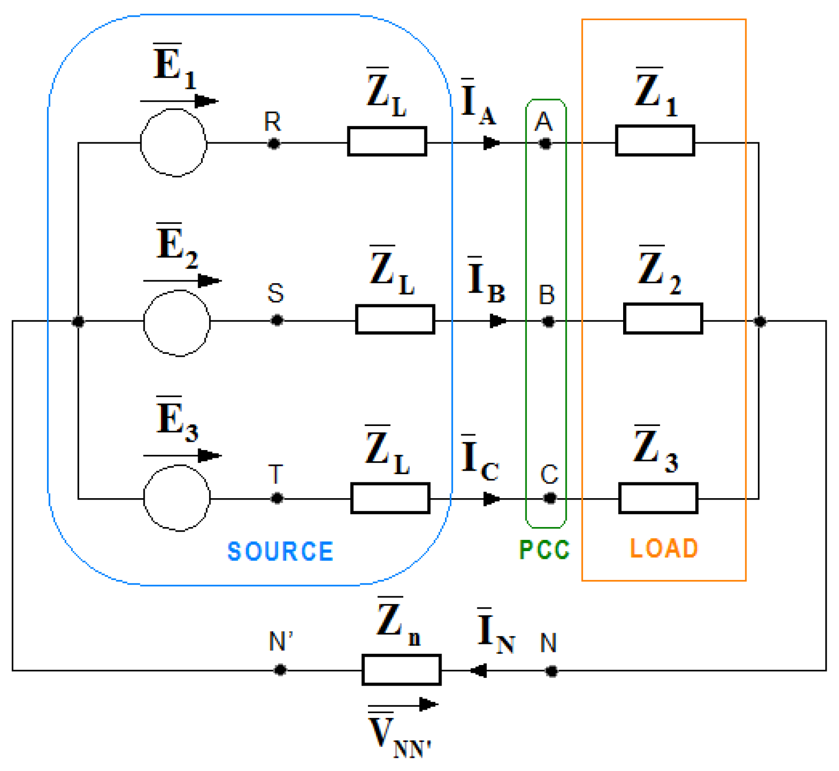
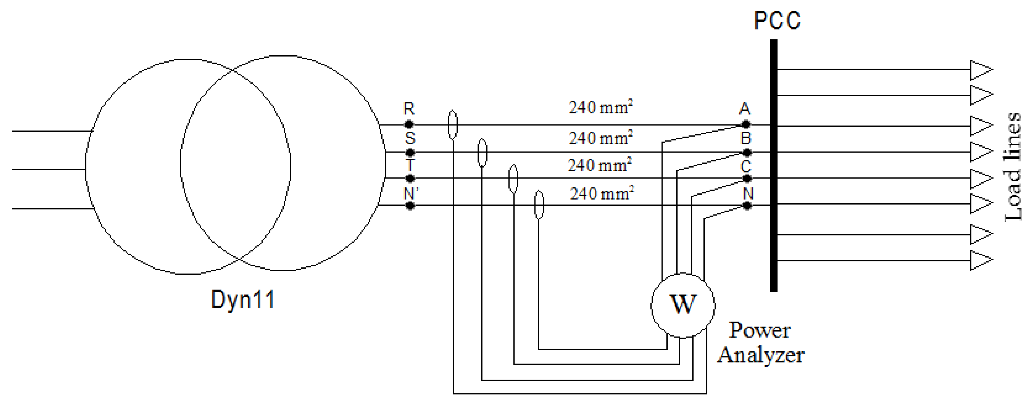
Let us consider a three-phase, four-wire power system similar to the one represented in Figure 1, with the source and the loads wye-configured, in which there is a neutral conductor that connects the neutral points of the source (N′) and the loads (N). The source impedances $Z_L$, represented in Figure 1, include both transformer impedances and line impedances in distribution networks. The instantaneous source,$p_s \left(t\right)$, and load, $p_{l }\left(t\right)$, powers are expressed as a function of the line-to-neutral source voltages ($v_{A{N}^{\prime }}, v_{B{N}^{\prime }}, v_{C{N}^{\prime }}$), and of the line-to-neutral load voltages ($v_{AN}, v_{BN}, v_{CN}$), and of the line currents ($i_A, i_B, i_C$), as follows:

$$p_s \left(t\right)=v_{A{N}^{\prime }}·i_A+v_{B{N}^{\prime }}·i_B+v_{C{N}^{\prime }}·i_C p_l\left(t\right)=v_{AN}·i_A+v_{BN}·i_B+v_{CN}·i_C,$$

(1)

These quantities have different values, in general, due to the neutral-displacement phenomenon [4,5,6]. The differences are more pronounced when there are unbalances and/or harmonic distortions in that system.

According to the Conservation of Energy Principle, the difference between the values of the instantaneous load and source powers must be attributed to the operation of the neutral conductor, whose instantaneous power is expressed as follows:

$$p_n\left(t\right)=p_l\left(t\right)-p_s\left(t\right)=-v_{N{N}^{\prime }}·\left(i_A+i_B+i_C\right)$$

(2)

where $v_{N{N}^{\prime }}$ is the voltage drop across the neutral conductor, also known as the neutral- displacement voltage, and the sum of the line currents is equal to the neutral current ($i_N=i_A+i_B+i_C$), according to Kirchhoff’s First Law.

We have called this power,$p_n\left(t\right)$, as the instantaneous neutral-displacement power [17], since it depends on the neutral-displacement voltage ($v_{N{N}^{\prime }}$) and identifies the energies that are manifested in three-phase systems due to the operation of the neutral conductor, in the event that this conductor exists, or caused by the action of the neutral path, in general. The term neutral path is habitually used when there is no neutral conductor, due to accidental breakage or because the loads are delta-configured.

The instantaneous powers that appear in the source and load due to the operation of the neutral conductor can be separately expressed by applying Fortescue’s theorem [19], namely,

$$v_{N{N}^{\prime }}=v_{A{N}^{\prime }0}-v_{AN0}$$

(3)

where $v_{A{N}^{\prime }0}$ and $v_{AN0}$ are the zero-sequence components of the line-to-neutral source and load voltages, respectively. Substituting the previous equation in (2), two components are deduced in the instantaneous neutral-displacement power,

$$p_n\left(t\right)=p_{nl}\left(t\right)+p_{ns}\left(t\right)=\left(v_{AN0}-v_{A{N}^{\prime }0}\right)·\left(i_A+i_B+i_C\right)$$

(4)

The first neutral-displacement power component,

$$p_{nl}\left(t\right)=v_{AN0}·\left(i_A+i_B+i_C\right),$$

(5)

identifies the energies that are manifested in the load by action of the neutral conductor (or the neutral path); while the second component,

$$p_{ns}\left(t\right)=-v_{A{N}^{\prime }0}·\left(i_A+i_B+i_C\right),$$

(6)

represents the energies supplied by the source due to the operation of the neutral conductor (or the neutral path).

The expressions of the instantaneous neutral-displacement powers as a function of the line currents ($i_A, i_B, i_C$), as observed in the previous equations, is more useful to study the effects of the neutral conductor than the use, in those equations, of the neutral current itself ($i_N$). Indeed, Equation (2) and the following determine that there may be energies in the phases of the source and load due to the action of the neutral path, even when there is no neutral conductor ($i_N=0$). Under these last conditions, the energies caused by the neutral path at the source and at the load are necessary to ensure compliance with the Conservation of Energy Principle and explain why the instantaneous load power can be different (generally higher) than the instantaneous source power.

The existing differences, in general, between the instantaneous source and load powers in the three-phase system of Figure 1 can also be observed between the values of the apparent powers of both subsystems. Just as the instantaneous powers identify the energies present in each subsystem, the apparent powers quantify the combined effects of those energies.

Numerous expressions of apparent power are well known in the Technical Literature. However, in our opinion, Buchholz’s apparent power [18] is more useful than the effective apparent power of A.E. Emanuel [20], included in the IEEE Standard 1459–2010 [21], to determine the effects of the neutral conductor in three-phase systems. This opinion is justified by the fact that Emanuel’s effective apparent power includes the neutral current in its expression, and, therefore, the power effects caused by the neutral conductor are included jointly with those due to the loads in the values measured by this apparent power. In contrast, the expression of Buchholz’s apparent power does not include any quantity of the neutral path, which makes it possible to determine the power effects of the neutral conductor separately from the source and the loads.

The apparent source and load powers ($S_s, S_l$) of the three-phase power system represented in Figure 1 have the following expressions, according to Buchholz:

$$S_s=\sqrt{\left(V_{A{N}^{\prime }}^2+V_{B{N}^{\prime }}^2+V_{C{N}^{\prime }}^2\right)·\left(I_A^2+I_B^2+I_C^2\right)} S_l=\sqrt{\left(V_{AN}^2+V_{BN}^2+V_{CN}^2\right)·\left(I_A^2+I_B^2+I_C^2\right)} ,$$

(7)

($V_{A{N}^{\prime }}, V_{B{N}^{\prime }}, V_{C{N}^{\prime }}$) are the RMS values of the line-to-neutral source voltages, ($V_{AN}, V_{BN}, V_{CN}$) are the RMS values of the line-to-neutral load voltages; and ($I_A, I_B, I_C$) are the RMS values of the line currents.

According to Fortescue’s theorem, the RMS values of the line-to-neutral source and load voltages are related to the RMS values of their respective symmetrical components as follows:

$$V_{A{N}^{\prime }}^2+V_{B{N}^{\prime }}^2+V_{C{N}^{\prime }}^2=3·\left(V_{A{N}^{\prime }+}^2+V_{A{N}^{\prime }-}^2+V_{A{N}^{\prime }0}^2\right) V_{AN}^2+V_{BN}^2+V_{CN}^2=3·\left(V_{AN+}^2+V_{AN-}^2+V_{AN0}^2\right),$$

(8)

where the sign (+) denotes the positive-sequence component, the sign (−) expresses the negative-sequence component, and (0) represents the zero-sequence component.

Likewise, the application of Fortescue’s theorem to the three-phase power system of Figure 1 also determines that $V_{A{N}^{\prime }+}=V_{AN+}$ and $V_{A{N}^{\prime }-}=V_{AN-}$. Therefore, the squared difference of the apparent load and source powers is reduced to the following expression:

$$S_l^2-S_s^2=3·\left(V_{AN0}^2-V_{A{N}^{\prime }0}^2\right)·\left(I_A^2+I_B^2+I_C^2\right)$$

(9)

Since the loads are usually more unbalanced and/or distorted than the sources, the RMS values of the zero-sequence component of the line-to-neutral load voltages are generally greater than those of the source ($V_{AN0}>V_{A{N}^{\prime }0}$), and the squared difference expressed by (9) would be positive in most power systems. For this reason, the neutral-displacement power ($S_n$) has been defined as follows [17]:

$$S_n=\sqrt{S_l^2-S_s^2}=\sqrt{3·\left(V_{AN0}^2-V_{A{N}^{\prime }0}^2\right)·\left(I_A^2+I_B^2+I_C^2\right) }$$

(10)

this power quantifies the power effects of the neutral conductor (or the neutral path) and also has two components,

$$S_{nl}=V_{AN0}·\sqrt{3·\left(I_A^2+I_B^2+I_C^2\right)} S_{ns}=V_{A{N}^{\prime }0}·\sqrt{3·\left(I_A^2+I_B^2+I_C^2\right)} ,$$

(11)

which determine the power effects of the neutral path on the load ($S_{nl}$) and on the source ($S_{ns}$), respectively.

Note that Equations (10) and (11) do not depend on the neutral current and, therefore, can be used in three-phase systems without a neutral conductor, which allows analyzing the effects of the operation of the neutral conductor from its nominal conditions to its breaking.

3. A Novel Parameter to Monitoring the Neutral Conductor Deterioration

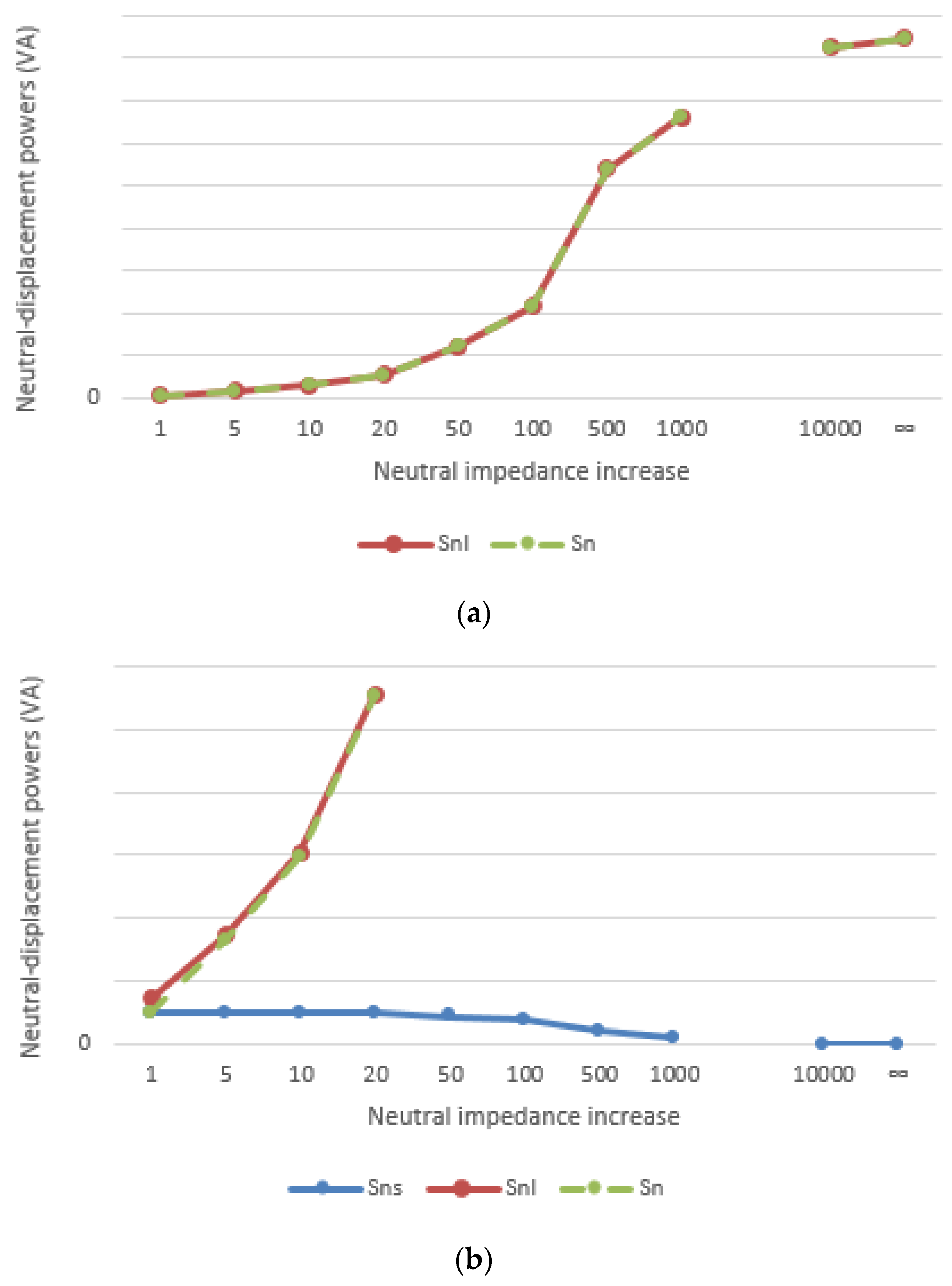
Figure 2a,b show a typical variation of the neutral-displacement power ($S_n$) and its effects on the load ($S_{nl}$) and on the source ($S_{ns}$), obtained at the fundamental frequency, during the breaking process of the neutral conductor of a three-phase power system.

It is noted that:

• $S_n$ and $S_{nl}$ have a strong increase in the early stages of the breaking process of the neutral conductor, which softens as the deterioration of the conductor is very great, and they reach their maximum value when the break is complete (Figure 2a).
• $S_n$ and $S_{nl}$ have very close values during practically the entire breaking process (Figure 2a) and only differ in the early stages of the process, when the deterioration of the neutral conductor is still small (Figure 2b), and
• the value of $S_{ns}$ remains practically invariable in the early stages of the breaking process and decreases progressively as the deterioration of the neutral conductor increases, until reaching a value equal to zero when that conductor has broken (Figure 2b).

According to the previously indicated data, it can be deduced that the growth of the value of the neutral-displacement power ($S_n$), or of its load component ($S_{nl}$), could be a more appropriate indicator for monitoring the neutral conductor’s deterioration than its source component ($S_{ns}$). On the other hand, the growth of $S_{nl}$ is easier to measure than that of $S_n$, since the value of $S_{nl}$ can be obtained using a measuring instrument (network analyzer) placed at the load, whereas the measurement of $S_n$ requires that the instrument be arranged in the neutral conductor, which is not always possible.

However, the values of $S_{nl}$ (as well as the values of $S_n$) change with the load power consumptions (i.e., the load impedances) and with the values of the source EMF. For this reason, a system for monitoring the neutral conductor condition based only on measuring the absolute value of $S_{nl}$ would not be useful, due to the difficulty in distinguishing whether the change in value of $S_{nl}$ is caused by a deterioration of the neutral conductor or by any load or source variation. To avoid this problem, some new monitoring parameters are defined below from the measurement of $S_{nl}$.

According to Equation (7), the load component of the neutral-displacement power ($S_{nl}$), defined by the first of the Equation (11), can be expressed as a function of the apparent load power ($S_l$), as follows:

$$S_{nl}=\frac{\sqrt{3}·V_{AN0}}{\sqrt{V_{AN}^2+V_{BN}^2+V_{CN}^2}}·S_l=\tau · S_l$$

(12)

where $V_{AN0}$ is the RMS value of the zero-sequence component of the line-to-neutral load voltages ($V_{AN}, V_{BN}, V_{CN}$).

The values of this dimensionless parameter,

$$\tau =\frac{S_{nl}}{S_l}=\frac{\sqrt{3}·V_{AN0}}{\sqrt{V_{AN}^2+V_{BN}^2+V_{CN}^2}},$$

(13)

also increase with the neutral conductor impedance, such as $S_{nl}$, and are also highly dependent on the load consumptions and the source EMF. However, the growth (∆τ) that the value of $\tau$ undergoes when the impedance of the neutral conductor increases is defined as:

$$\Delta \tau =\frac{\tau }{{\tau }_o},$$

(14)

where τ is the value corresponding to each impedance of the neutral conductor ($Z_n$), and τ_o its initial value, corresponding to the nominal conditions of that conductor ($Z_{no}$), is hardly affected by the load power consumptions and the source EMF, as will be verified in Section 5. For this reason, we consider that ∆τ is an adequate parameter to monitor the condition of the neutral conductor.

4. Procedure for Monitoring the Neutral Conductor Condition

This section describes a procedure for monitoring the neutral conductor condition, which is based on the measurement of the parameter ∆τ, defined by (14), using the values of the fundamental-frequency voltages, at the point of common coupling (PCC) between the source and loads of the three-phase distribution networks (Figure 1).

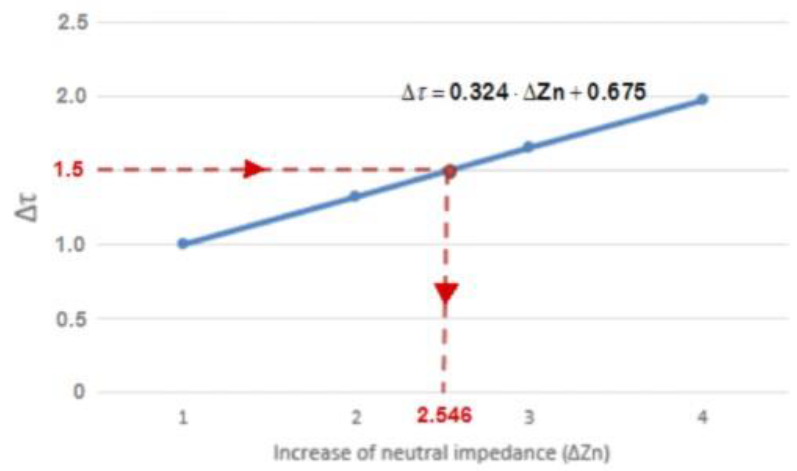
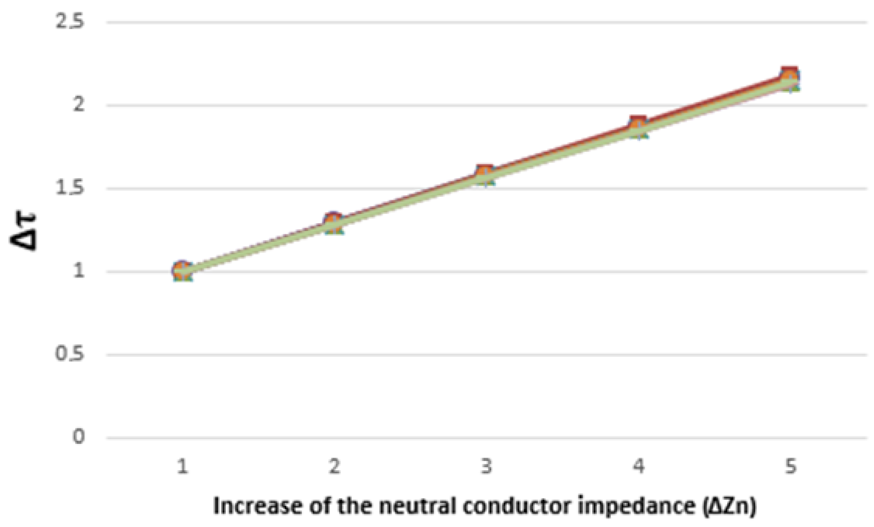
From Figure 2a,b, it can be seen that the growth of the parameter ∆τ for small increases (not greater than 10 times) of the impedance of the neutral conductor ($\Delta Z_n=Z_n/Z_{no}$) can be approximated to a line of equation (Figure 3):

$$\Delta \tau =A·\Delta Z_n+B$$

(15)

as will be verified in Section 5, in which the values of the coefficients A and B depend on the nominal impedances of the neutral conductor ($Z_{no}$), and are hardly affected by the values of the source EMF and by the load consumptions.

The nominal impedances of the neutral conductors of three-phase distribution networks can be calculated based on the values of resistance and reactance, for each section and unit length of the cables, as defined by the Spanish Standard UNE 20460-5-523:2004 [22] (Equivalent to IEC 60364-5-523:1999 MOD). For unipolar cables, the most common sections in three-phase distribution networks, the values of the conductor impedances per unit length are those indicated in

Table 1. Resistances, reactances and impedances, per unit length, corresponding to each section of single-pole cables of distribution networks, according to the Standard UNE 20460-5-523:2004.

Section (mm2)	Resistance Rn (mΩ/m)	Reactance Xn (mΩ/m)	Impedance Zn (mΩ/m)
			Module	Angle ($°$)
25	0.889	0.106	0.8953	6.80
35	0.841	0.101	0.847	6.85
50	0.473	0.101	0.4837	12.05
70	0.328	0.0965	0.3342	16.39
95	0.236	0.0975	0.2553	22.45
120	0.188	0.0939	0.21	26.54
150	0.153	0.0928	0.1789	31.24
185	0.123	0.0908	0.1529	36.43
240	0.0943	0.0902	0.1305	43.73
300	0.0761	0.0895	0.1175	49.63

. The values of coefficients A and B in Equation (15) are summarized in

Table 2. Values of coefficients $A$ and $B$ for the $\Delta \tau$ growth line, corresponding to each section and length of the neutral conductors of distribution networks with the generic load and transformer no-load secondary voltages of 395 V.

Section (mm2)	NEUTRAL CONDUCTOR LENGTH
	4 m		8 m		12 m		16 m
	A	B	A	B	A	B	A	B
25	0.5063	0.4858	0.6333	0.3649	0.6671	0.3323	0.6897	0.3113
35	0.4949	0.4977	0.6178	0.3785	0.6667	0.3333	0.6876	0.3119
50	0.3521	0.6377	0.5124	0.4828	0.586	0.4093	0.6281	0.3719
70	0.2614	0.731	0.4213	0.573	0.5113	0.4855	0.5638	0.4324
95	0.2096	0.7847	0.3536	0.641	0.4431	0.5522	0.5056	0.4917
120	0.1774	0.818	0.3099	0.6851	0.3992	0.595	0.4585	0.541
150	0.1563	0.8412	0.2762	0.72	0.3625	0.6325	0.4217	0.5752
185	0.1381	0.8598	0.2456	0.7516	0.3251	0.671	0.3854	0.6118
240	0.1241	0.8744	0.2194	0.7792	0.2923	0.7056	0.3462	0.6533
300	0.1142	0.8847	0.2027	0.7962	0.271	0.7276	0.324	0.675

for different lengths and sections of the neutral conductor. These values of coefficients A and B have been obtained by representing the values of the parameter ∆τ obtained with the support of the simulation software for Circuit Design Suite, Multisim version 14.1 [23] in a three-phase distribution network, with a transformer of 395 V line-to-line no-load secondary voltages and a generic star load with impedances: ${\overline{Z}}_1=23.126\angle -5.9°\mathsf{\Omega }$, ${\overline{Z}}_2=22.728\angle -2.7°\mathsf{\Omega }$ and ${\overline{Z}}_3=19.873\angle -9.2°\mathsf{\Omega }$.

From Table 2, the following properties of coefficients A and B of the $\Delta \tau$ growth line are noted:

• for a given length of the neutral conductor, the coefficient A decreases as the section increases, while, on the contrary, the coefficient B increases with the section of the conductor,
• for a given section of neutral conductor, the coefficient A increases with the length of the conductor, while the coefficient B decreases,
• for neutral conductors of the same section, the values of A and B corresponding to intermediate lengths to those indicated in Table 2 can be obtained by interpolation, the error being smaller the greater the length of the conductor, and
• for neutral conductors of the same length, the coefficients A for two consecutive sections have very close values, and the same can be said for the coefficients B. So the values of A and B of both sections can be used interchangeably without making a big error.

The procedure for monitoring the condition of the neutral conductor has the following steps:

Step 1. Characterization of the neutral conductor, introducing the values of the coefficients A and B of the ∆τ growth line, obtained from Table 2 according to its length and section (Table 2).

Step 2. Measurement of the RMS values of the fundamental-frequency line-to-neutral voltages ($V_{AN}, V_{BN}, V_{CN}$), and of their zero-sequence component ($V_{AN0}$), by means of a power analyzer located at the point of common coupling (PCC) between the source and the loads.

Step 3. Obtaining the value of τ and its variation ∆τ, using Equations (13) and (14), respectively.

Step 4. Determination of the state of the neutral conductor, according to the value of $\Delta Z_n$ obtained as follows

$$\Delta Z_n=\frac{\Delta \tau -B}{A}$$

(16)

Using this procedure on a line of 16 m long and 300 mm² in section, the coefficients A and B are according to Table 2: $A=0.324, B=0.675$. According to Equation (16), it is observed that if the measured value of $\Delta \tau =1$, the neutral conductor is operating on its nominal conditions ($\Delta Z_n=1$ and $Z_n=Z_{no}=0.00188\angle 43.69°\mathsf{\Omega }$). However, if the value measured by the analyzer is $\Delta \tau =1.5$, it follows from Equation (16) that $\Delta Z_n=$ 2.546 (Figure 3), that is, the impedance of the neutral conductor has increased 2.546 times with respect to its nominal value ($Z_{no}$), indicating a significant deterioration of that conductor, which may be an early indication of the beginning of its breakage.

5. Practical Application

In this section, through a practical application on one of the transformation houses of the Low Voltage distribution network of an Electric Company located in the town of Vinalesa (Valencia, Spain), it will be verified that:

(1)

the measurement of the values of the fundamental-frequency line-to-neutral load voltages, or of their zero-sequence component, does not constitute an adequate procedure for the early detection of the neutral conductor breakage,

(2)

nor is the measure, at the fundamental-frequency, of the parameter τ, defined by (13), but

(3)

its variation (∆τ), expressed by (14), is a good surveillance parameter, since its growth with the deterioration of the neutral conductor always follows the same pattern for a given network, regardless of the value of the transformer no-load secondary voltages and of the load consumptions.

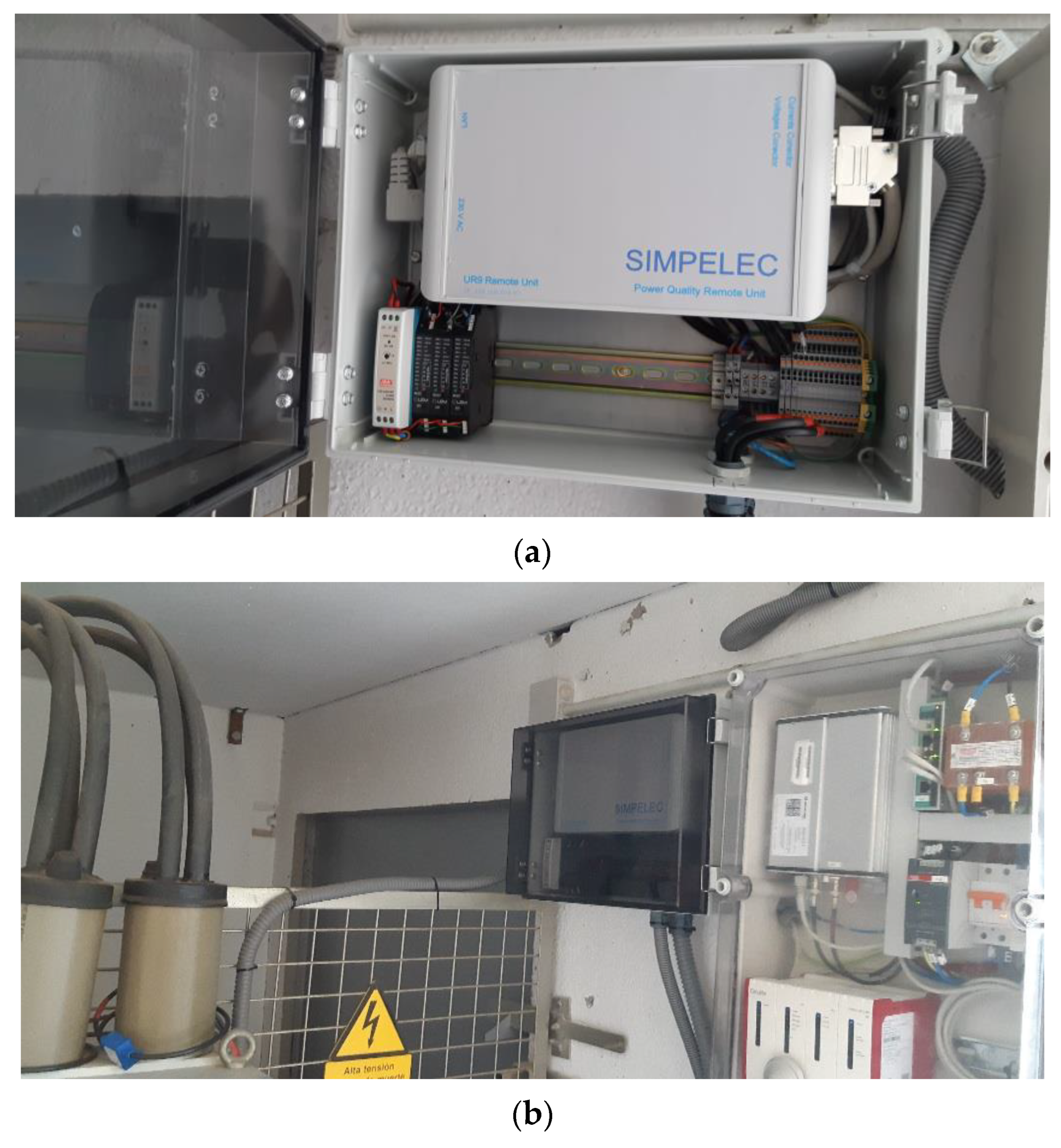
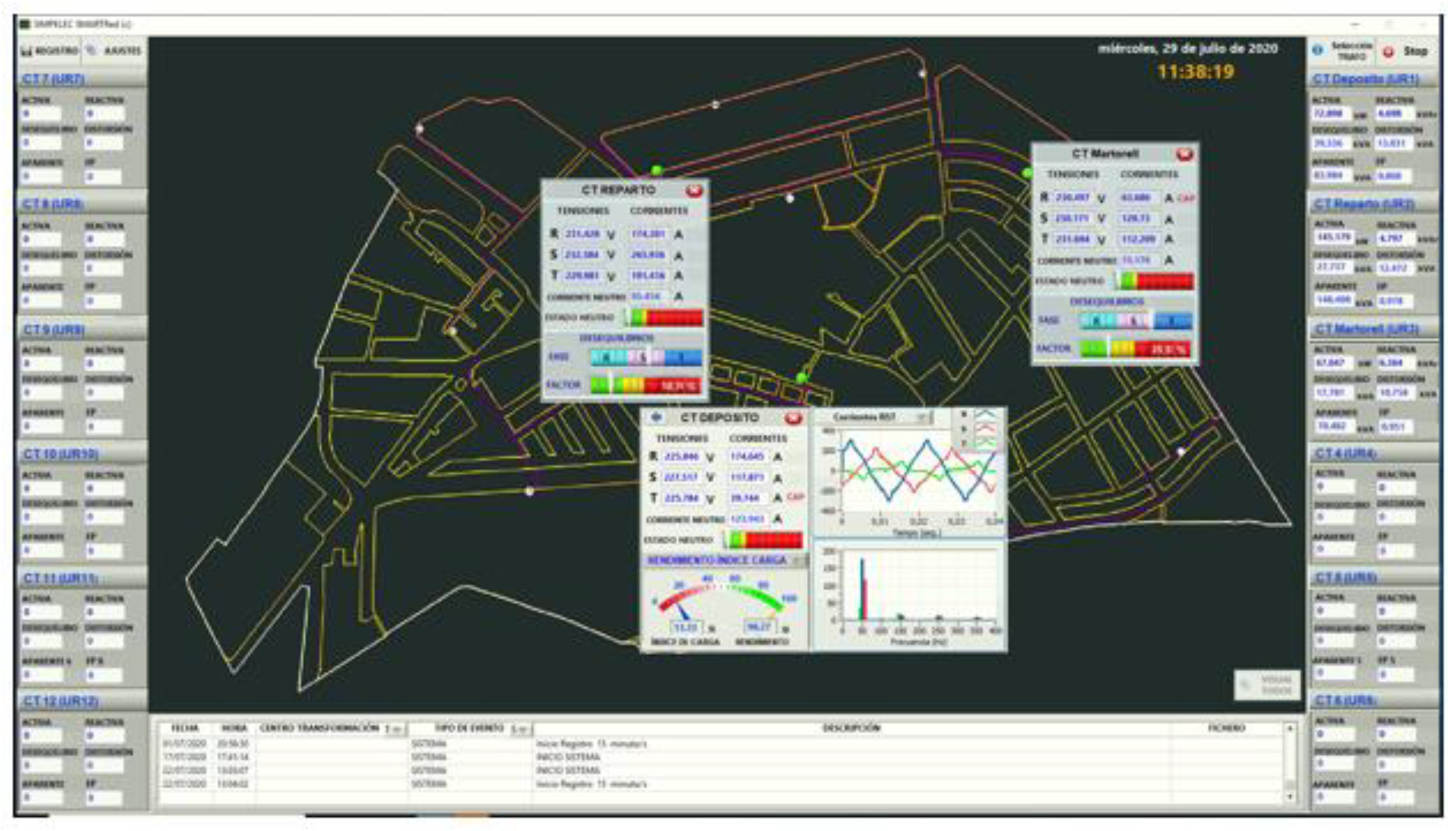
We have a power analyzer, granted under the name of SIMPELEC (Figure 4a,b), for real-time monitoring the neutral conductor, among many other parameters of the Vinalesa distribution network. This instrument is a remote unit that sends the voltage and current signals registered at the point of common coupling (PCC) of each transformation house to a centralized unit, in which the SIMPELEC-SMARTRed software [24] calculates the different quantities and parameters of the network. 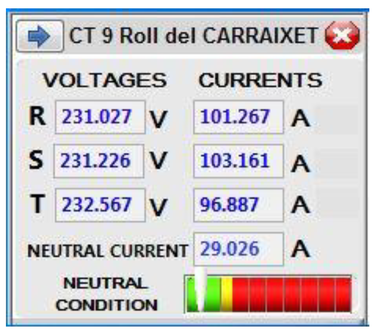Currently, we have four of these analyzers installed in as many transformation houses as there are in the aforementioned distribution network (Figure 5). The study of the deterioration and breakage process of the neutral conductor is carried out in this section for one of these transformation houses. Specifically, the transformation house under study is CT9, called Roll del Carraixet.

The monitoring of the neutral conductor of the main line of the CT9 is currently carried out by the SIMPELEC system using the procedure indicated in Section 4. The values of the coefficients A and B of the ∆τ growth equation ($\Delta \tau =A·\Delta Z_n+B$) are determined from Table 2 according to the main line dimensions (length and section), described in Section 5.1. From the real-time registers sent by the SIMPELEC analyzer, the values of ∆τ are determined, according to Equations (13) and (14), by the SIMPELEC-SMARTRed software. Then, the values of $\Delta Z_n$, corresponding to each of the measured values of ∆τ, are calculated according to Equation (16). Any value of $\Delta Z_n>1$ implies a deterioration of the neutral conductor with respect to its nominal conditions.

The neutral conductor condition of the main line of each transformation house is presented in a LabVIEW screen, as the one represented in Figure 6, by the SIMPELEC-SMARTRed software. In the lower part of this screen, a cursor indicates the state of the neutral conductor on a bar with the colors: green (normal operation), yellow (slight deterioration), and red (important deterioration and risk of breakage).

Despite the fact that the SIMPELEC system is capable of detecting the deterioration of the neutral conductor, we have not been able to verify it in practice since no defect has occurred in the neutral conductors of the lines analyzed during the measuring campaign (cursor over the green zone, Figure 6). Due to the dangerous damages that the disconnection of the neutral conductor could cause to the customers of the distribution network, the neutral breaking process in the main line of the CT9 transformation house has been analyzed by simulation, with the support of the commercial simulation software Multisim [23]. For that:

-

Firstly, we have verified that the results obtained with Multisim are the same as those measured by the SIMPELEC analyzer in the nominal conditions of the neutral conductor.

-

Secondly, we have analyzed the results provided by Multisim, when the neutral impedance has been progressively increased, for simulating the breaking process of the neutral conductor.

5.1. Nominal Features of the Analyzed Three-Phase Distribution Network

Table 3. CT9 transformer nominal features.

Nominal Power (kVA)	Primary Voltage (V)	No-Load Secondary Voltage (V)	Copper Losses (W)	No-Load Losses (W)	Short-Circuit Voltage (%)
630	20,000	395	6500	1300	4

summarizes the nominal features of the Dyn11 three-phase transformer of the distribution network used for the practical application (Figure 7).

The analyzed network has a main line (Figure 7) of 240 mm² in section and 12 m long, which connects the secondary transformer terminals ($R, S, T, N\prime$) and the PCC ($A, B, C, N$).

The managers of the distribution network have set the transformer no-load secondary line-to-line voltages at 395 V. However, the Multisim simulation software allows analyzing the operation of the breaking process of the neutral conductor with other no-load secondary voltages (390 V and 400 V) different from the actual regulated value.

The loads fed by this transformer are fairly balanced. For the study of the neutral conductor breakage process, we have selected three of the power consumptions registered by the SIMPELEC analyzer. The values of the complex impedances corresponding to these consumptions are, at the fundamental-frequency (50 Hz), those indicated in

Table 4. Fundamental-frequency complex impedances of the three analyzed loads.

	LOAD 1		LOAD 2		LOAD 3
	MODULE (Ω)	ANGLE ($°$)	MODULE (Ω)	ANGLE ($°$)	MODULE (Ω)	ANGLE (°)
A-phase	1.3790	39.637	1.6087	43.596	1.94838	47.22
B-phase	1.34045	39.257	1.49788	41.805	1.7945	41.405
C-phase	1.16144	43.539	1.37419	47.797	1.91206	47.587

.

5.2. Effects of the Neutral Conductor Deterioration on the PCC Line-to-Neutral Voltages and Their Zero-Sequence Component

The surveillance of the RMS values of the fundamental-frequency line-to-neutral load voltages and of their zero sequence component are indirect procedures traditionally used to detect the neutral conductor condition.

Table 5. Variation of the fundamental-frequency RMS values of the PCC line-to-neutral voltages and their zero-sequence component, when the neutral conductor impedance increases ($\Delta Z_n$ ) and the transformer no-load secondary voltages are 395 V.

$\Delta {\mathit{Z}}_{\mathit{n}}$	LOAD 1				LOAD 2				LOAD 3
	${\mathit{V}}_{\mathit{A}\mathit{N}}$	${\mathit{V}}_{\mathit{B}\mathit{N}}$	${\mathit{V}}_{\mathit{C}\mathit{N}}$	${\mathit{V}}_{\mathit{A}\mathit{N}0}$	${\mathit{V}}_{\mathit{A}\mathit{N}}$	${\mathit{V}}_{\mathit{B}\mathit{N}}$	${\mathit{V}}_{\mathit{C}\mathit{N}}$	${\mathit{V}}_{\mathit{A}\mathit{N}0}$	${\mathit{V}}_{\mathit{A}\mathit{N}}$	${\mathit{V}}_{\mathit{B}\mathit{N}}$	${\mathit{V}}_{\mathit{C}\mathit{N}}$	${\mathit{V}}_{\mathit{A}\mathit{N}0}$
1	226.48	226.46	226.06	0.147	226.64	226.58	226.32	0.079	226.84	226.80	226.85	0.070
2	226.49	226.49	226.02	0.189	226.65	226.60	226.30	0.101	226.83	226.79	226.87	0.090
3	226.50	226.53	225.98	0.231	226.65	226.62	226.28	0.124	226.83	226.77	226.89	0.110
4	226.51	226.56	225.94	0.274	226.66	226.63	226.26	0.147	226.82	226.76	226.91	0.131
5	226.52	226.59	225.89	0.316	226.66	226.65	226.24	0.169	226.81	226.75	226.93	0.151
50	226.91	227.79	224.31	1.966	226.80	227.36	225.39	1.074	226.49	226.24	227.75	0.981
500	228.25	232.32	218.64	7.955	227.44	230.14	222.04	4.662	225.04	224.03	231.49	4.743
$\infty$	229.16	325.75	214.60	12.293	228.05	232.41	219.28	7.604	223.53	221.94	235.27	8.532

summarizes the RMS values of the fundamental-frequency line-to-neutral voltages ($V_{AN}, V_{BN}, V_{CN}$) and their zero-sequence component ($V_{AN0}$), measured at the (PCC) of the analyzed distribution network, during the process of deterioration and breakage of the neutral conductor of the main line, for the no-load voltage of 395 V, and for each of the three loads indicated in Table 5. The RMS values of the PCC voltages corresponding to $\Delta Z_n=1$ have been recorded, at the fundamental frequency, by the SIMPELEC analyzer under the nominal conditions of the neutral conductor. The remaining PCC voltage values indicated in

Table 6. Fundamental-frequency values of parameters τ and ∆τ as a function of the increment of the neutral conductor impedance ($\Delta Z_n$ ) for the three analyzed loads and transformer no-load secondary line-to-line voltages of 390 V.

$\Delta {\mathit{Z}}_{\mathit{n}}$	LOAD 1		LOAD 2		LOAD 3
	$\mathit{\tau }·{10}^{-3}$	$\Delta \mathit{\tau }$	$\mathit{\tau }·{10}^{-3}$	$\Delta \mathit{\tau }$	$\mathit{\tau }·{10}^{-3}$	$\Delta \mathit{\tau }$
1	0.6409	1	0.3429	1	0.3041	1
2	0.8257	1.288340	0.4420	1.289005	0.3922	1.289707
3	1.0123	1.579484	0.5421	1.580927	0.4814	1.583032
4	1.1991	1.871140	0.6425	1.873724	0.5709	1.877343
5	1.3856	2.162159	0.7428	2.166229	0.6604	2.171654

have been obtained for different values of $\Delta Z_n$ (from 2 to infinity) to simulate the breaking process of the neutral conductor, using the Multisim software.

Observing Table 5, it can be deduced that:

• The RMS values of the fundamental-frequency line-to-neutral voltages can increase, decrease, or be maintained in each phase of the PCC during the breaking process of the neutral conductor, although these variations may be different in each phase, depending on the values of the loads.
• With slightly unbalanced loads, such as those indicated in Table 4, the growth of the RMS values of the PCC fundamental-frequency line-to-neutral voltages may be undetectable for the over-voltage protection relays, even with very large damage to the neutral conductor. This fact can be verified in Table 6, for the second load, in which the over-voltages reach values of only 232.41 V, when the neutral conductor has already broken. The over-voltages on loads 1 and 3 are somewhat higher than on load 2 (235.75 V and 235.21 V, respectively) and could activate the over-voltage relays, but also when the neutral conductor is broken.
• The RMS values of the zero-sequence component of the PCC fundamental-frequency line-to-neutral voltages ($V_{AN0}$) increase with the deterioration of the neutral conductor, but these values are different for each load.

Based on the previous observations, it could be concluded that the procedure for monitoring the state of the neutral conductor based on the observation of the RMS values of the fundamental-frequency line-to-neutral voltages is not suitable. These voltages have different values depending on the load. For slightly unbalanced loads, the neutral conductor may break without the over-voltages being high enough to activate the protection relay. The procedure based on watching the values of the zero-sequence component of the fundamental-frequency line-to-neutral voltages is not appropriate to detect neutral conductor deteriorations because, even though this quantity always increases with the neutral conductor impedance, their values depend markedly on the loads.

5.3. Monitoring of the Neutral Conductor Condition Based on the Measurement of the Parameter $\Delta \tau$

In this section, we study whether the parameter τ or its variation ∆τ are suitable for monitoring the deterioration of the neutral conductor. For this, the effects on the values of these parameters caused by changes in the loads and in the transformer secondary EMF are analyzed. Likewise, it is analyzed how the variations in the ∆τ growth lines affect the value of the increase in the neutral conductor impedance ($\Delta Z_n$), calculated according to the procedure established in Section 4, in the early stages of the breaking process of the neutral conductor.

The study is carried out with the support of the Multisim simulation software, for the first stages of the process of deterioration and breakage of the neutral conductor used in this practical application, whose dimensions, indicated in Section 5.1, are: 12 m long and 240 mm² in section. The effects caused by the loads on the parameters τ and ∆τ are analyzed using the three loads indicated in Table 5 and subsequently compared with the generic load (${\overline{Z}}_1=23.126\angle -5.9°\mathsf{\Omega }$, ${\overline{Z}}_2=22.728\angle -2.7°\mathsf{\Omega }$, ${\overline{Z}}_3=19.873\angle -9.2°\mathsf{\Omega }$), described in Section 4, to obtain Table 2. The effects of the secondary EMF values have been analyzed using the transformer’s actual regulation voltages of 395 V, as well as two other possible regulation values (390 V and 400 V) that can be used through the Multisim.

5.3.1. Effects of Loads and Supply Voltages on the Parameters τ and ∆τ

Table 6,

Table 7. Fundamental-frequency values of parameters τ and ∆τ as a function of the increment of the neutral conductor impedance ($\Delta Z_n$ ) for the three analyzed loads and transformer no-load secondary line-to-line voltages of 395 V.

$\Delta {\mathit{Z}}_{\mathit{n}}$	LOAD 1		LOAD 2		LOAD 3
	$\mathit{\tau }·{10}^{-3}$	$\Delta \mathit{\tau }$	$\mathit{\tau }·{10}^{-3}$	$\Delta \mathit{\tau }$	$\mathit{\tau }·{10}^{-3}$	$\Delta \mathit{\tau }$
1	0.6510	1	0.3483	1	0.3089	1
2	0.8355	1.283410	0.4472	1.283951	0.3969	1.284882
3	1.0218	1.569585	0.5472	1.571059	0.4860	1.573325
4	1.2085	1.856375	0.6475	1.859029	0.5754	1.862739
5	1.3949	2.142703	0.7477	2.146713	0.6648	2.152153

and

Table 8. Fundamental-frequency values of parameters τ and ∆τ as a function of the increment of the neutral conductor impedance ($\Delta Z_n$ ) for the three analyzed loads and transformer no-load secondary line-to-line voltages of 400 V.

$\Delta {\mathit{Z}}_{\mathit{n}}$	LOAD 1		LOAD 2		LOAD 3
	$\mathit{\tau }·{10}^{-3}$	$\Delta \mathit{\tau }$	$\mathit{\tau }·{10}^{-3}$	$\Delta \mathit{\tau }$	$\mathit{\tau }·{10}^{-3}$	$\Delta \mathit{\tau }$
1	0.6611	1	0.3537	1	0.3222	1
2	0.8454	1.278778	0.4526	1.279615	0.4124	1.279950
3	1.0315	1.560278	0.5524	1.561775	0.5038	1.563625
4	1.2180	1.842384	0.6526	1.845066	0.5956	1.848541
5	1.4042	2.124036	0.7528	2.128357	0.6874	2.133457

summarize the values of the parameters τ and ∆τ, as the value of the impedance of the neutral conductor ($Z_n$) increases from one to five times its nominal value ($Z_{no}$). The values of τ and ∆τ have been calculated, in these early stages of deterioration of the neutral conductor, by applying Equations (13) and (14), respectively, with the values of the fundamental-frequency line-to-neutral load voltages, obtained by the Multisim simulation software for each analyzed load and secondary EMF.

From Table 6, Table 7 and Table 8, it can be deduced that:

• For each load, the values of the parameter τ, expressed by (13), increase as the impedance of the neutral conductor ($\Delta Z_n$) increases.
• The values of τ are very slightly affected by the supply voltages, but they are very dependent on the values of the loads. For this reason, the parameter τ cannot be used to monitor the state of the neutral conductor.
• As the impedance of the neutral conductor ($\Delta Z_n$) increases, the values of the parameter ∆τ, defined by (14), are practically independent of the loads and are very slightly affected by the values of the secondary EMF. For this reason, ∆τ can be an effective for monitoring the state of the neutral conductor.

These properties of the parameter ∆τ can be confirmed based on the variations of its values with the increase in the neutral conductor impedance ($\Delta Z_n$), indicated in Table 6, Table 7 and Table 8. It is verified that the variations of ∆τ as a function of $\Delta Z_n$ can be adjusted to straight lines, whose equations are shown in

Table 9. Growth lines of ∆τ as a function of the neutral conductor impedance increment ($\Delta Z_n$ ) for the three analyzed loads and transformer no-load secondary line-to-line voltages of 390 V, 395 V and 400 V.

EMF (V)	LOAD 1	LOAD 2	LOAD 3
390	$0.2907·\Delta Z_n+0.7082$	$0.2917·\Delta Z_n+0.7068$	$0.2931·\Delta Z_n+0.7051$
395	$0.2858·\Delta Z_n+0.7129$	$0.2869·\Delta Z_n+0.7116$	$0.2882·\Delta Z_n+0.71$
400	$0.2812·\Delta Z_n+0.7176$	$0.2822·\Delta Z_n+0.7163$	$0.2836·\Delta Z_n+0.7145$

for each of the loads and transformer secondary EMF.

Comparing the growth lines of ∆τ, specific to each load and transformer secondary EMF (

Table 10. Calculated values of $\Delta Z_n$ using the $\Delta \tau$ growth lines of Table 2 and Table 10, for the analyzed loads, no-load secondary line-to-line voltages and several $\Delta \tau$ values.

No-Load Secondary Voltages (V)	TYPE OF LOAD	$\Delta \mathit{\tau }$
		1.00	1.25	1.50	2.00
390	LOAD 1	1.00	1.86378	2.72377	4.44375
	LOAD 2	1.00	1.86219	2.71923	4.43332
	LOAD 3	1.00	1.85909	2.71204	4.41795
395	GENERIC LOAD	1.00	1.86247	2.71775	4.42833
	LOAD 1	1.00	1.87928	2.75402	4.50350
	LOAD 2	1.00	1.87661	2.74799	4.49076
	LOAD 3	1.00	1.87370	2.74115	4.47606
400	LOAD 1	1.00	1.89331	2.78236	4.56045
	LOAD 2	1.00	1.89121	2.77711	4.54890
	LOAD 3	1.00	1.88822	2.76975	4.53279

), with the generic growth line of ∆τ, obtained from Table 2 for a generic load very different from those indicated in Table 5,

$$\Delta \tau =0.2923·\Delta Z_n+0.7056$$

it is observed that all of them have coefficients A and B with very similar values. That is, the growth of ∆τ as the deterioration of the neutral conductor increases is very little affected by the load and secondary EMF changes.

5.3.2. Errors Caused by the Changes in Loads and Secondary EMF on the $\Delta Z_n$ Calculation

This section determines the relative errors in the calculation of the neutral impedance increments ($\Delta Z_n$) that would result from using the expression of the generic growth line of ∆τ instead of the expressions of the growth lines of ∆τ specific to each load and secondary EMF. These errors are determined for the neutral conductor of the main line of the distribution network used in the practical application, whose dimensions are 12 m long and 240 mm² in section. Hence, the generic growth line is $\Delta \tau =0.2923·\Delta Z_n+0.7056$ (Table 2) and the specific growth lines of ∆τ are presented in Table 10.

Figure 8 graphically represents all the growth lines of ∆τ, both the generic one obtained from Table 2 and the specific ones corresponding to the different loads and secondary EMF (Table 9). It is observed in Figure 8 that these growth lines are practically superimposed, which suggests the errors in the calculation of the increase in the neutral conductor impedance ($\Delta Z_n$) according to the proposed procedure should not be important.

Indeed, Table 10 summarizes the values of $\Delta Z_n$ calculated for four values of ∆τ (1, 1.25, 1.5, and 2), which result from applying Equation (16) with the coefficients A and B corresponding to the growth lines of ∆τ indicated in Table 2 and Table 10.

The errors that would result when using the generic growth line of $\Delta \tau$ (Table 2) instead of the specific ones in Table 9 are summarized in Table 10. Thus, for example, it can be seen that if the transformer were feeding load 3, with transformer no-load secondary voltages of 395 V, and $\Delta \tau =1.5$, the calculated value of the increase in neutral conductor impedance would be $\Delta Z_n=2.74779$ (

Table 11. Relative errors, in %, in calculating the increase of the neutral conductor impedance ($\Delta Z_n$ ) using the $\Delta \tau$ generic growth line obtained from Table 2.

No-Load Secondary Voltages (V)	TYPE OF LOAD	$\Delta \mathit{\tau }$
		1.00	1.25	1.50	2.00
390	LOAD 1	0	0.070	0.221	0.347
	LOAD 2	0	−0.015	0.054	0.113
	LOAD 3	0	−0.182	−0.211	−0.235
395	LOAD 1	0	0.895	1.317	1.669
	LOAD 2	0	0.753	1.100	1.390
	LOAD 3	0	0.599	0.853	1.066
400	LOAD 1	0	1.629	2.322	2.897
	LOAD 2	0	1.520	2.137	2.651
	LOAD 3	0	1.364	1.877	2.305

), using the specific growth line of ∆τ (load 3 and 395 V). However, if, under the above conditions (load 3, 395 V and $\Delta \tau =1.5$), we had used the generic growth line of ∆τ, the calculated value of the increase in the impedance of the neutral conductor, had been $\Delta Z_n=2.71775$. That is, the use of the generic growth line instead of the specific one for load 3, both with transformer no-load secondary voltages of 395 V and $\Delta \tau =1.5$, would originate an absolute error in the measure of $\Delta Z_n$ of only 0.03004 and a relative error of 0.853% (Table 11). Both errors are small enough not to seriously disturb the monitoring of the state of the neutral conductor.

Table 11 summarizes the relative errors, in %, that would result in the calculation of $\Delta Z_n$ if the generic growth line of ∆τ (Table 2) was used instead of the growth lines of ∆τ specific of each load and secondary EMF (Table 9), for different values of ∆τ (1, 1.25, 1.5 and 2). It is observed that:

• there are no errors in the calculation of $\Delta Z_n$ when $\Delta \tau =1$, that is, when the neutral conductor operates in its nominal conditions,
• for each load and secondary EMF, the errors in the calculation of $\Delta Z_n$ increase according to the value of ∆τ increases, and
• the largest relative error observed in the determination of $\Delta Z_n$ has been only 2.897%, obtained for values of $\Delta \tau =2$, when the distribution network feeds load 1 and the transformer secondary EMF are 400 V (Table 11). It is noted that in those conditions there is a significant deterioration of the neutral conductor ($\Delta Z_n>4$, Table 10).

The small errors in the calculation of $\Delta Z_n$, observed in Table 11, suggest that it is possible to determine the increase in the neutral impedance, with a great approximation to the real increase, using the generic growth line of ∆τ, defined by Table 2, without the need to use the specific growth lines for each load and secondary EMF.

6. Conclusions

The indirect procedure for real-time monitoring of the state of the neutral conductor in three-phase distribution networks based on monitoring the growth of the novel parameter ∆τ in loads, has been described in this paper. Its results have been compared in the distribution network of an actual Electric Company with those obtained by two traditional procedures, based on monitoring the fundamental-frequency line-to-neutral load voltages and their zero-sequence components.

Traditional procedures are not very suitable. It has been verified that the RMS values of the fundamental-frequency line-to-neutral voltages can grow a lot in some load phase (over-voltages) and their zero-sequence component always increases with the deterioration of the neutral conductor, but these values are highly dependent on the loads. For this reason, an increase in the values of these quantities can be due to either the deterioration of the neutral conductor or any change in the loads. Likewise, the over-voltages caused by the slightly unbalanced loads caused by the deterioration of the neutral conductor may be negligible and incapable of activating the protection relays.

The new parameter τ, established in this paper according to Equation (13), is a relationship between the previous fundamental-frequency load voltages. Hence, its use for monitoring the state of the neutral conductor has the same drawbacks as the two traditional procedures mentioned above. However, the variation of this parameter with respect to its initial value ($\Delta \tau =\tau /{\tau }_o$) is an effective parameter, in our opinion, for monitoring the deterioration and breakage of the neutral conductor, for the following reasons:

• $\Delta \tau$ grows with the increasing of the neutral conductor impedance ($\Delta Z_n$) according to a straight line of equation $\Delta \tau =A·\Delta Z_n+B$, during the early stages of neutral conductor deterioration (generally up to $\Delta Z_n=10$);
• the values of the coefficients A and B are determined by the length and section of the neutral conductor, as indicated in Table 2;
• the load variations and the changes in the secondary EMF of the transformers of the distribution networks affect very slightly the values of the coefficients A and B.

Considering these properties of the parameter ∆τ, the procedure established in this paper allows calculating in real-time the increase in the impedance of the neutral conductor ($\Delta Z_n$), with great approximation, by substituting the values of ∆τ, measured in the loads at the fundamental frequency, in the expression (16), using the values of A and B defined by Table 2. The procedure:

• is effective and can be applied to any low-voltage distribution network, even with slightly unbalanced loads, simply by knowing the dimensions (length and section) of the neutral conductor;
• does not introduce errors in the calculation of $\Delta Z_n$, when the neutral conductor is operating in its nominal conditions, that is, for a measured value of $\Delta \tau =1$;
• in the presence of significant deterioration of the neutral conductor ($\Delta Z_n>4$), the load variations introduce errors of less than 2% in the calculation of the real value of $\Delta Z_n$;
• in the presence of significant deterioration of the neutral conductor ($\Delta Z_n>4$), the combined effects of changes in loads and secondary EMF give rise to maximum errors of less than 3% in the calculation of the real value of $\Delta Z_n$.

The small errors in the calculation of $\Delta Z_n$, which occur because of changes in the loads and/or in the transformer secondary EMF, are acceptable for monitoring the state of the neutral conductor, in our opinion. That is because we do not intend to know the exact value of the impedance of the neutral conductor, but only to detect its deterioration sufficiently in advance to allow the rapid activation of the protection devices, avoiding damage to the loads.

In the future, we aim to apply the novel parameter (∆τ), defined in this paper, to the detection of lack of symmetry in distribution transformers, whether caused by accidental faults in their windings, or due to manufacturing defects.

7. Patents

The following patent and registered software are resulting from the work reported in this manuscript:

• León-Martínez, V.; Montañana-Romeu, J. Procedure and device for the determination of the state of the neutral conductor in an electrical installation. Spanish Patent ES2588260B2. Granted: 28 April 2017.
• Montañana-Romeu, J.; León-Martínez, V. SIMPELEC-SMARTRed: Software for Monitoring Electric Power Distribution Networks. Universitat Politècnica de València. Registered: 29 October 2021.