Article

Research on the Optimal Control Strategy for the Maximum Torque per Ampere of Brushless Doubly Fed Machines

School of Electrical and Information Engineering, Tianjin University, No. 92 Weijin Road, Tianjin 300072, China
*
Author to whom correspondence should be addressed.
Machines 2023, 11(4), 422; https://doi.org/10.3390/machines11040422
Submission received: 21 February 2023 / Revised: 9 March 2023 / Accepted: 23 March 2023 / Published: 25 March 2023
(This article belongs to the Special Issue Advanced Data Analytics in Intelligent Industry: Theory and Practice)

Abstract

:
This paper presents an optimization strategy for a brushless doubly fed motor (BDFM) to achieve the maximum torque per ampere (MTPA). This method resolves the issue of high stator currents in slip frequency vector feedback linearization control (SFV-FLC) during both no-load and light-load conditions. Firstly, the paper establishes a reduced-order state-space (SS) model of the BDFM in arbitrary rotating reference coordinates. Secondly, the expression of BDFM is obtained after the control motor rotor field orientation. To ensure a minimal stator current at a specific torque, this paper constructs an auxiliary function based on Lagrange’s theorem, which forces the control motor stator current derivative to be zero, resulting in the MTPA criterion. Finally, the superiority of the MTPA optimization algorithm proposed in the paper is validated through simulation experiments.

1. Introduction

The brushless doubly fed motor (BDFM) [1,2,3] is an innovative type of motor capable of operating in multiple ways. It offers adjustable speed and power factors and features a low-capacity frequency converter. Moreover, the BDFM eliminates the need for brushes and slip rings, which significantly reduces maintenance costs and failure rates [4]. Given these advantages, scientific researchers have demonstrated a keen interest in the BDFM.
The BDFM has a more intricate structure than typical asynchronous motors, resulting in a more complex modeling and controller design. Therefore, simplifying the system modeling and designing effective optimal [5] control strategies presents a significant challenge. Currently, the vector control (VC) method and direct torque control (DTC) [6,7] method of BDFM have both been extensively studied. In comparison to VC [8,9,10,11], DTC utilizes the stator flux and torque as control variables in the static reference frame. Therefore, no sophisticated coordinate transformation is required, and the response time is faster. However, DTC utilizes a hysteresis structure, resulting in fluctuating torque and a high harmonic current content.
Recently, to realize high-performance precise decoupling control and enhance the system reliability [12] of the BDFM, scholars at home and abroad have conducted extensive and in-depth research on VC with different magnetic field orientations. A rotor-field-oriented vector control scheme was proposed based on the dual synchronous coordinate system in [5]. The BDFM is divided into two subsystems which carry out independent field-oriented control. This not only makes the derivation more complicated but also prevents the actual decoupling of the system. For an in-depth analysis, it was necessary to [5,13] further analyzed the load performance of the BDFM using this control method and carried out a simulation verification. A unified reference frame model is set out in [8] to streamline control by rotating the two associated variables of the rotor in the same direction, using the conjugate relationship between the rotor currents of the power motor (PM) and the control motor (CM). When the arbitrary flux is chosen for orientation, all the model variables are DC values. From among these studies, [9,10,11] realized the control of the power and speed based on the stator field orientation. From the perspective of the derivation of the mathematical model and the difficulty of control, the mathematical model [14,15,16,17] based on the unified synchronous coordinate system is more practical.
The difference between the BDFM and asynchronous motors is that the decoupling of the system cannot be achieved except through rotor field orientation. At the same time, considering that the current inner loop with the faster response is often designed in the actual control application, [18] established the SS model and the decoupling control method of the BDFM under the power supply of the current source. Although [18] solved the above existing problems, when the BDFM is running at no-load and light-load conditions, the stator current of the method [14] is large, which leads to an increase in copper loss and lower efficiency of the machine and the probability of system faults [19].
To improve the operation efficiency of the BDFM, the control trajectory is close to the optimal trajectory of the MTPA. In recent years, the MTPA [20] control of the single motor [21] has been studied extensively. However, compared with the single motor, both the BDFM’s modeling and the controller design are more challenging. Only Hamidreza Mosaddegh et al. [22,23] have conducted relevant research on BDFMs. To simplify the system model [24] and reduce the difficulty of system control, the equivalent circuit of the BDFM is equivalent to the traditional DFM. On this basis, the MTPA control of the BDFM is studied using stator-field-oriented control and feedback linear control. The phase angle corresponding to the minimum stator current is obtained by looking up the table. However, the MTPA lookup table method can only look up the phase angle of the corresponding current, which not only has certain constraints but also has a low calculation accuracy and occupies a specific storage space. Therefore, to compensate for the deficiency of [22], based on the SS model and the electromagnetic torque equation, the use of Lagrange’s theorem to force the derivative of the stator current to zero ensures the realization of the MTPA strategy. The rotor flux corresponding to the minimum value of the stator current amplitude is obtained by calculating the electromagnetic torque and the slip speed. Finally, the BDFM control system is realized by combining the MTPA control with the SFV-FLC (slip frequency vector feedback linear control) [25].
This paper continues to optimize the SFV-FLC based on the recent research [25]. Its innovations mainly include the following two aspects: on the one hand, the rotor flux command value in the SFV-FLC is directly established by humans; however, the MTPA optimal control is based on the online calculation of the command values of torque and speed to obtain the flux command corresponding to the minimum stator current. On the other hand, the load torque in the SFV-FLC is not arbitrary. It is necessary to calculate the torque range in which the BDFM can run stably according to the command value of the rotor flux and the speed. Only when the value is taken within the torque boundary can the stable operation of the BDFM be guaranteed; however, the load torque of the MTPA optimal control can be established arbitrarily, and it will adjust the given value of the rotor flux in real time according to the load torque and the speed command. As long as the inverter capacity is large enough, the BDFM can always work in a stable state. The optimal MTPA methods not only reduce the loss of the system but also result in improved system operating efficiency and effectively avoid winding insulation breakdown faults [26].
The paper is organized as follows: Section 2 presents the reduced-order state-space model of the BDFM. Section 3 details the derivation process of the MTPA optimal control method under the control machine’s rotor field orientation. Section 4 offers simulations and experimental verification of the MTPA-(SFV-FLC) control method. Section 5 provides the conclusion of the paper.

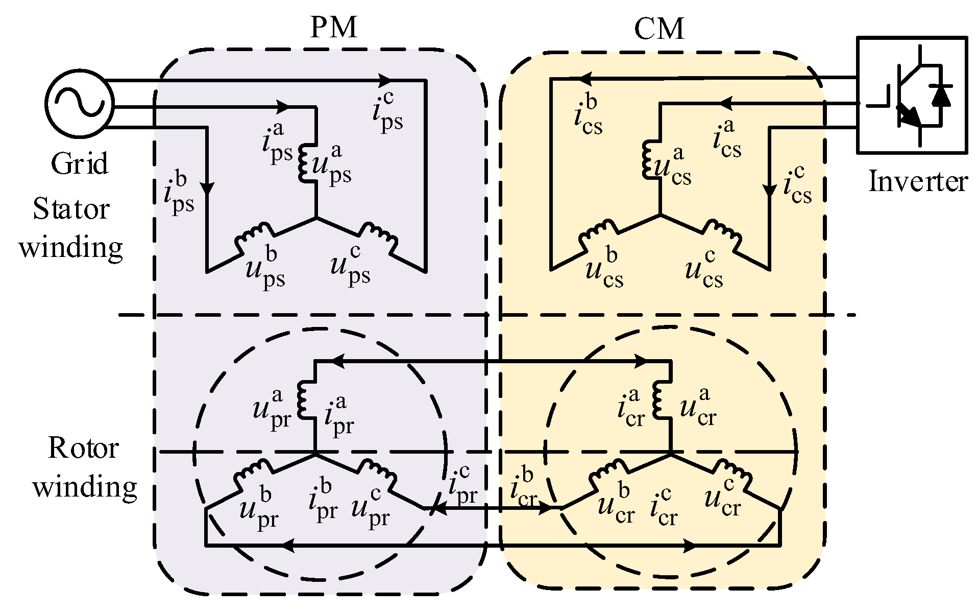
2. Reduced-Order State-Space Equations for BDFM

As shown in Figure 1, the BDFM is composed of two cascaded induction motors connected in series. The induction motor connected to the grid is defined as the PM, and the induction motor connected to the inverter is defined as the CM; two sets of rotor windings are connected in reverse order. There is no magnetic coupling between the stator windings of the PM and the CM, only the electrical coupling between the rotor windings.
The mathematical model of the BDFM in the rotor reference frame is obtained by taking the CM as a reference [25]:
u ¯ p s d q = ( r p s j p p ω r l p s ) i ¯ p s d q j p p ω r l p m i r d q + l p s i ¯ ˙ p s d q + l p m i ˙ r d q u c s d q = ( r c s + j p c ω r l c s ) i c s d q + j p c ω r l c m i r d q + l c s i ˙ c s d q + l c m i ˙ r d q 0 = r r i r d q + l p m i ¯ ˙ p s d q + l c m i ˙ c s d q + l r i ˙ r d q
where the PM and CM are indicated by the subscripts p and c, respectively. The time derivative is shown by the superscript “.”, and s and r denote the stator and rotor, respectively. Resistance, inductance and mutual inductance are each represented by r, l and lm. Vectors in the complex form are used to express the variables u, i and Ψ. The rotor resistance and the rotor inductance are represented by r r = r c r + r p r , l r = l c r + l p r , respectively. The conjugate and negative conjugate are indicated by the superscripts “*” and “-”, respectively.
Next, we simplify Equation (1) into the following state-space equation:
x ˙ dq = A dq x dq + B dq u dq
where
A dq = 1 Δ [ M ( r ps + j p p ω r l ps ) l pm l cm ( r cs + j p c ω r l cs ) l cs l pm r r + j p p ω r M l pm j p c ω r l pm l cm 2 l pm l cm ( r ps + j p p ω r l ps ) N ( r cs + j p c ω r l cs ) l cm l ps r r + j p p ω r l cm l pm 2 j p c ω r N l cm l cs l pm ( r ps + j p p ω r l ps ) l cm l ps ( r cs + j p c ω r l cs ) l cs l ps r r j p p ω r l cs l pm 2 + j p c ω r l ps l cm 2 ] B dq = 1 Δ [ M l pm l cm l pm l cm N l cs l pm l cm l ps ] , x dq = [ i ¯ ps dq i cs dq i r dq ] , u dq = [ u ¯ ps dq u cs dq ] Δ = l ps l cs l r l cs l pm 2 l ps l cm 2 , M = l cs l r l cm 2 , N = l ps l r l pm 2
Considering that all the state variables in the rotor coordinate system are AC quantities, which is not conducive to control, it is necessary to continue to perform the following rotation transformation: x mt = e j λ x dq . The following is the BDFM state-space equation:
x ˙ mt = A mt x mt + B mt u mt
where
A mt = 1 Δ [ M ( r ps + j p p ω r l ps ) j Δ λ ˙ l pm l cm ( r cs + j p c ω r l cs ) l pm l cm ( r ps + j p p ω r l ps ) N ( r cs + j p c ω r l cs ) j Δ λ ˙ l cs l pm ( r ps + j p p ω r l ps ) l cm l ps ( r cs + j p c ω r l cs ) l cs l pm r r + j p p ω r Ml pm j p c ω r l pm l cm 2 l cm l ps r r + j p p ω r l cm l pm 2 j p c ω r Nl cm l cs l ps r r + j ( p p ω r l cs l pm 2 + p c ω r l ps l cm 2 Δ λ ˙ ) ] B mt = 1 Δ [ M l pm l cm l pm l cm N l cs l pm l cm l ps ] , x mt = [ i ¯ ps mt i cs mt i r mt ] , u mt = [ u ¯ ps mt u cs mt ]
To eliminate the effect of the CM stator voltage, the new CM rotor flux is given as:
ψ cr mt = l cm i cs mt + l cr i r mt
where l cr = l pr + l cr ( l pm 2 / l ps ) .
Substituting Equation (4) into Equation (3) simplifies the problem to obtain a reduced-order state-space model:
x ˙ mt = A mt x mt + B mt u mt
where
A mt = [ r ps l ps + j ( p p ω r λ ˙ ) r ps l pm l ps l cr l pm l ps 2 ( r ps j p p ω r l ps ) H l ps 2 l cr j λ ˙ ] , B mt = [ 1 r ps l cm l pm l ps l cr l pm l ps Hl cm l ps 2 l cr ] , x mt = [ ψ ¯ ps mt ψ cr mt ] , u mt = [ u ¯ ps mt i cs mt ]
The electromagnetic torque equation is:
T e = p p l pm l cm l ps l cr I m { ψ ¯ ps mt ( i cs mt ) * } + p c l cm l cr Im { ( ψ cr mt ) * i cs mt } p p l pm l ps l cr Im { ψ ¯ ps mt ( ψ cr mt ) * }
where Im stands for the imaginary part of the operation, the conjugate transformation is represented by “*”, and the moment of inertia is represented by J.

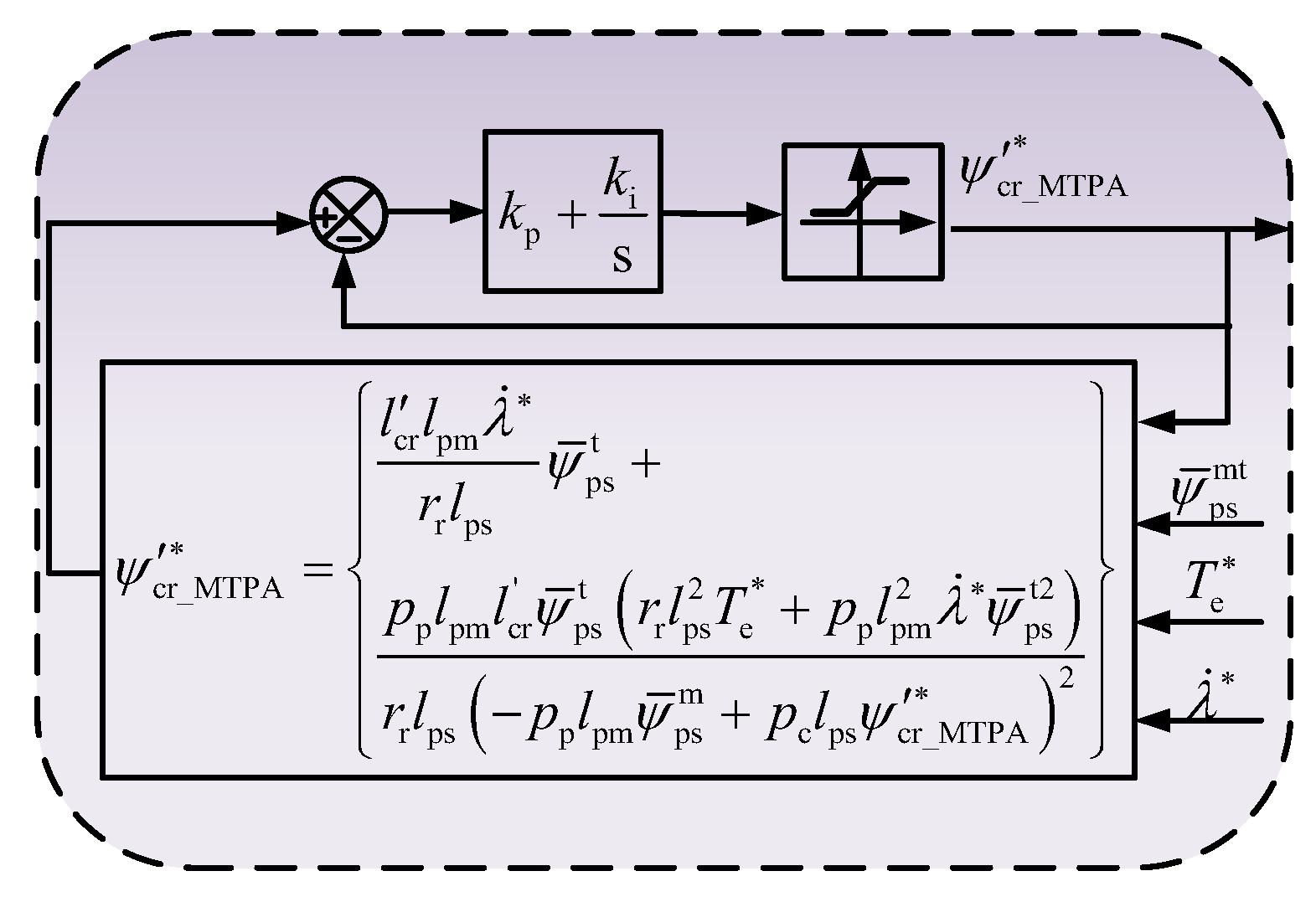
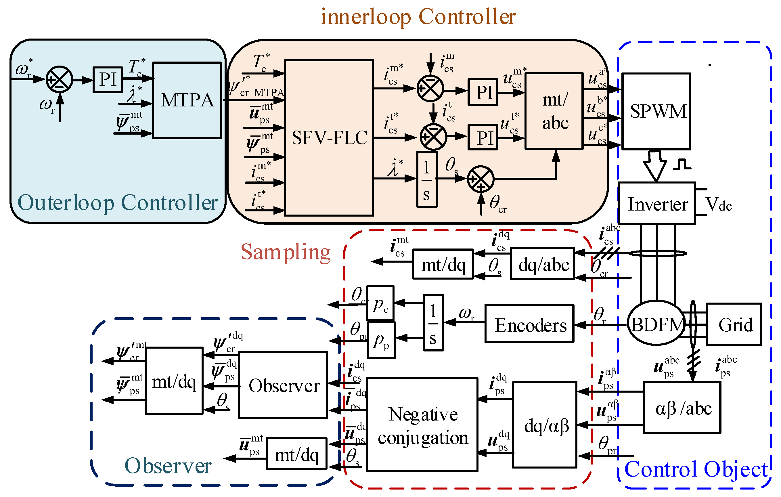
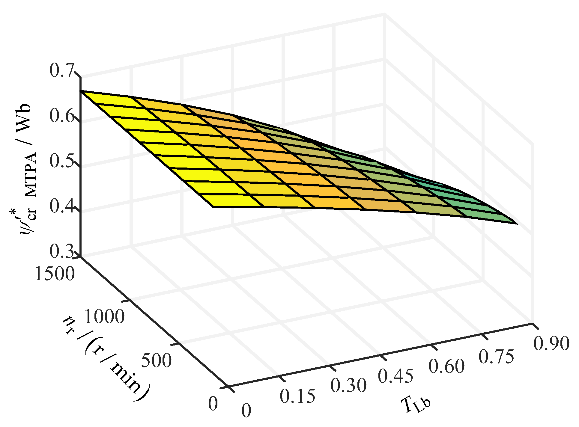
3. Description of MTPA-(SFV-FLC) Optimal Control Strategy

Selecting the rotor flux defined by Equation (4) for field orientation, we obtain:
ψ cr mt = ψ cr m + j ψ cr t = ψ cr + j 0
Substituting (7) into (5), (6) can be written as:
i cs m = l ps 2 l cr Hl cm ψ ˙ cr + 1 l cm ψ ˙ cr + l pm l cr l ps H l cm ( u ¯ ps m     p p ω r ψ ¯ ps t ) l pm l cr r ps H l cm ψ ¯ ps m
λ ˙ = l pm l ps p p ω r ψ ¯ ps m + r ps l pm l ps 2 ψ ¯ ps t l pm l ps u ¯ ps t + H l cm l ps 2 l cr i cs t ψ cr
i cs t = T e p p l pm l cm l ps l cr ψ ¯ ps t i cs m + p p l pm l cr l ps ψ ¯ ps t ψ cr l cm l cr ( p c ψ cr l pm l ps p p ψ ¯ ps m )
To ensure that the system has a solution, it needs to satisfy:
( p c ψ cr * l pm l ps p p ψ ¯ ps m ) 0 and ψ cr * > p p l pm p c l ps ψ ¯ ps m
To enhance the operational efficiency of the BDFM and align its control trajectory with the optimal trajectory of the MTPA, the MTPA control criterion is derived using Lagrange’s theorem, and its performance is discussed. The results indicate that the MTPA control of the BDFM may minimize the stator current of the BDFM, in addition to reducing the stator copper loss and the inverter’s capacity and enhancing the power factor and operating efficiency of the entire system.
Based on the above analysis, the torque Equation (10) and the CM stator current amplitude are selected as constraints:
{ i cs _ min = i cs m 2 + i cs t 2 T e = p p l pm l ps l cr ψ ¯ ps t ψ cr + ( p c l cm l cr ψ cr p p l pm l cm l ps l cr ψ ¯ ps m ) i cs t + p p l pm l cm l ps l cr ψ ¯ ps t i cs m
Then, we construct auxiliary functions:
F = i cs m 2 + i cs t 2 + ζ ( p p l pm l ps l cr ψ ¯ ps t ψ cr + p p l pm l cm l ps l cr ψ ¯ ps t i cs m + ( p c l cm l cr ψ cr p p l pm l cm l ps l cr ψ ¯ ps m ) i cs t T e )
where ζ is the Lagrange multiplier.
Next, we find the partial derivatives of i cs m , i cs t and ζ respectively. Then:
F i cs m = 2 i cs m + ζ ( p p l pm l cm l cr l ps ψ ¯ ps t ) = 0
F i cs t = 2 i cs t + ζ l cm l cr ( p p l pm l ps ψ ¯ ps m + p c ψ cr ) = 0
F ζ = p p l pm l ps l cr ψ ¯ ps t ψ cr   + p p l pm l cm l ps l cr ψ ¯ ps t i cs m   T e   + ( p c l cm l cr ψ cr p p l pm l cm l ps l cr ψ ¯ ps m ) i cs t   = 0
According to Equations (14) and (15), we observe that:
  i cs m i cs t = p p l pm ψ ¯ ps t p p l pm ψ ¯ ps m + p c l ps ψ cr
By combining the state-space Equations (8) and (9), the expressions for the CM stator current are obtained:
  i cs m = 1 l cm ψ cr λ ˙ l pm l cr r r l ps l cm ψ ¯ ps t
We substitute Equation (18) into (10) to obtain the torque current:
i cs t = l cr ( r r l ps 2 T e + λ ˙ p p l pm 2 ψ ¯ ps t 2 ) r r l ps l cm ( p p l pm ψ ¯ ps m + p c l ps ψ cr )
From Equations (18) and (19), we can observe:
i cs m i cs t = ( r r l ps ψ cr λ ˙ l pm l cr ψ ¯ ps t ) ( p p l pm ψ ¯ ps m + p c l ps ψ cr ) l cr ( r r l ps 2 T e + λ ˙ p p l pm 2 ψ ¯ ps t 2 )
Combine (17) and (20) to obtain the MTPA criterion:
( r r l ps ψ cr l cr l pm λ ˙ ψ ¯ ps t ) ( p p l pm ψ ¯ ps m + p c l ps ψ cr ) 2 p p l pm l cr ψ ¯ ps t ( r r l ps 2 T e + p p l pm 2 λ ˙ c ψ ¯ ps t 2 ) = 0
The MTPA algorithm is based on T e * calculated by the speed loop, λ calculated by the SFV-FLC, and the stator flux ψ ¯ ps mt obtained by the observer, ψ cr _ MTPA is obtained by solving Equation (21). The properties of the problem show that ψ cr _ MTPA has only one positive real number solution (so the negative limit of the PI regulator should be zero to obtain a positive real number solution), which can be obtained by feedback iteration. Thus, this is obtained by (21):
ψ cr _ MTPA * = l cr l pm λ ˙ r r l ps ψ ¯ ps t + p p l pm l cr ψ ¯ ps t ( r r l ps 2 T e * + p p l pm 2 λ ˙ ψ ¯ ps t 2 ) r r l ps ( p p l pm ψ ¯ ps m + p c l ps ψ cr _ MTPA * ) 2
Accordingly, the feedback system shown in Figure 2 is constructed, and to obtain a solution without static error, the PI regulator is used. ψ cr _ MTPA is a steady-state solution of the system depicted in Figure 2, and the following steady-state solutions are close to it:
ψ cr _ MTPA * ( ψ cr _ MTPA * + l cr l pm λ ˙ r r l ps ψ ¯ ps t + p p l pm l cr ψ ¯ ps t ( r r l ps 2 T e * + p p l pm 2 λ ˙ ψ ¯ ps t 2 ) r r l ps ( p p l pm ψ ¯ ps m + p c l ps ψ cr _ MTPA * ) 2 ) = 1 2 p p p c l pm l cr ψ ¯ ps t ( r r l ps 2 T e * + p p l pm 2 λ ˙ ψ ¯ ps t 2 ) r r ( p p l pm ψ ¯ ps m + p c l ps ψ cr _ MTPA * ) 3
From Equation (11), we observed that the denominator of (23) is always greater than zero. Thus, as long as (23) is always less than zero near the steady-state solution (actually near 1), the negative feedback system can be formed. Therefore, guaranteed stability can be ensured by the feedback system shown in Figure 2, and the desired solution can be obtained.
Figure 3 shows the MTPA-(SFV-FLC) optimal control block diagram of the BDFM. T e * is generated by the speed loop. The MTPA online computing generates ψ cr _ MTPA . To avoid the drift of open-circuit integrals, the stator current model of two motors in the rotor coordinate system is used to obtain the PM stator flux [25]. The PM stator flux in the m-t reference frame can be obtained by rotation transformation. T e * , λ and ψ ¯ ps mt are added into Figure 2 to obtain ψ cr _ MTPA , and then they are combined with the SFV-FLC [25] to complete the control.
In order to show the rule that the MTPA control changes with speed and torque, the CM rotor flux is solved offline by combining (8)–(10) and the MTPA Equation (21). Based on Table 1, ψ cr _ MTPA is obtained by Matlab/Simulink, and TLb represents the per unit value of torque. TLb= TL/TN, as depicted in Figure 4, Figure 5 and Figure 6. The rotor flux drops with increasing torque for a constant machine speed. When the torque remains constant, the CM rotor flux similarly decreases as the speed increases.

4. Simulation Experiment Results

To validate the effectiveness and reliability of the MTPA-(SFV-FLC) control scheme, in this paper, Matlab/Simulink is used to construct a BDFM simulation experiment platform. The motor flux needs to be observed during the control process, and the flux observation model in the rotor coordinate system is as follows:
{ ψ ¯ ps dq = l pm l cm s ( r r + l r s ) i cs dq + l ps ( r r + l cr s ) ( r r + l r s ) i ¯ ps dq ψ cr dq = l cm ( r r + l pm s ) ( r r + l r s ) i cs dq l cr l pm s ( r r + l r s ) i ¯ ps dq

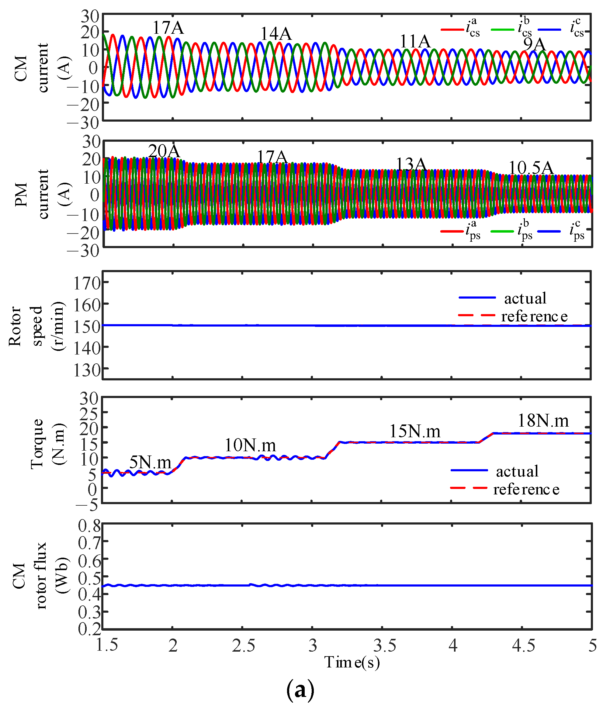
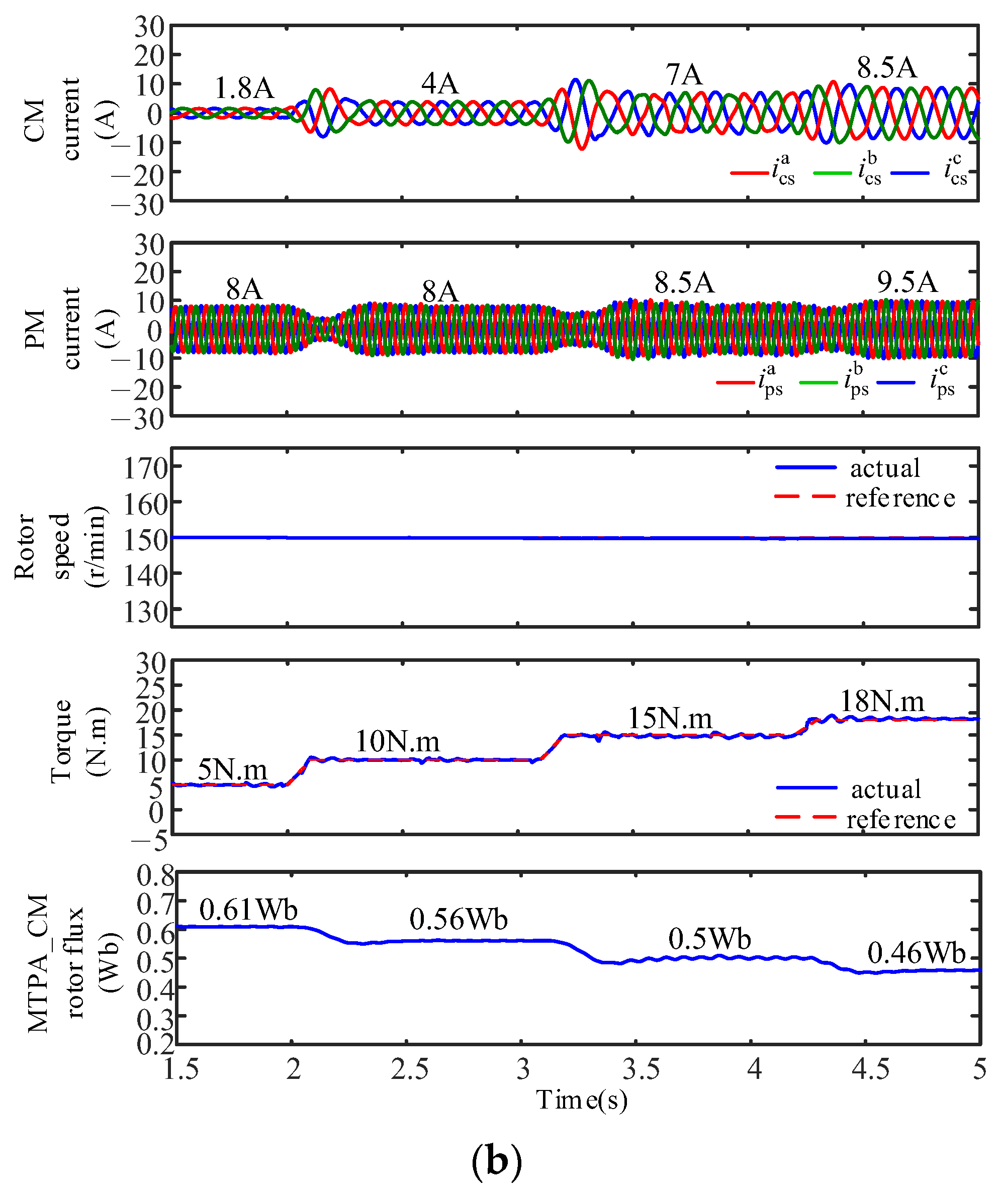
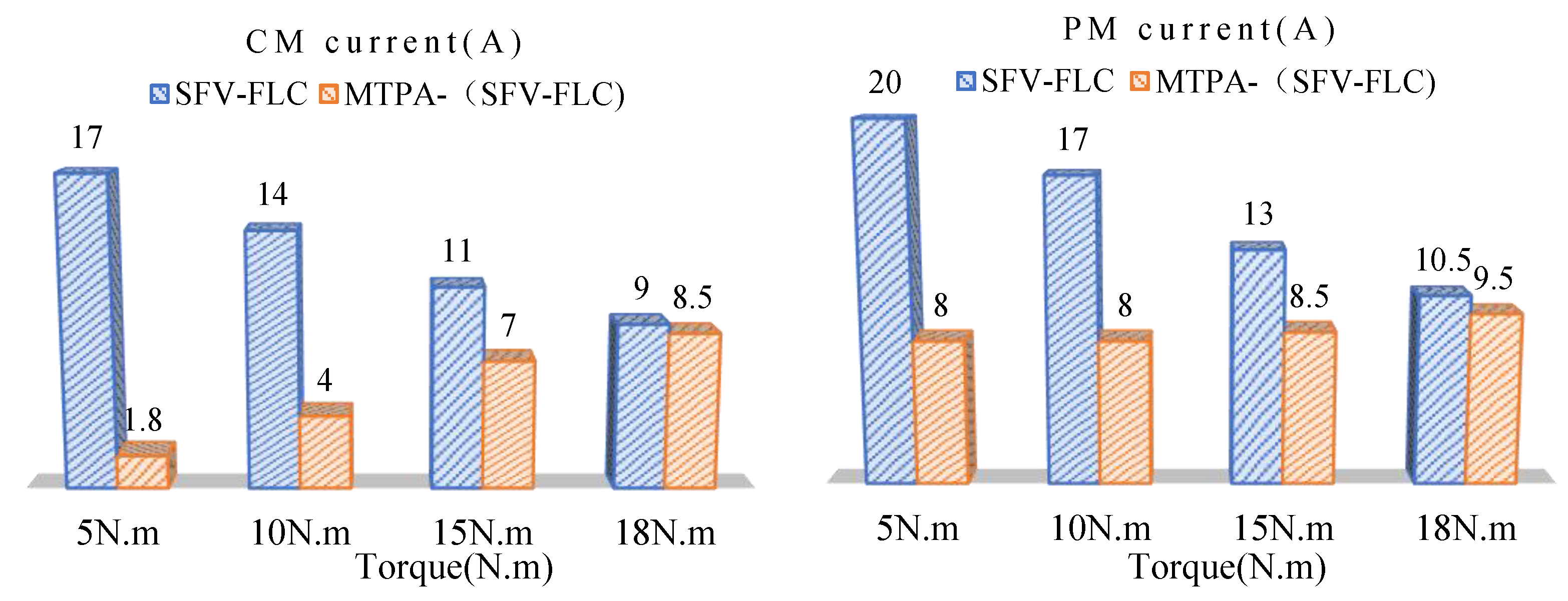
4.1. Verification of Dynamic Tracking Performance

Simulation experiment conditions: The PM is supplied with 66 V/15 Hz according to the constant voltage frequency ratio of 220 V/50 Hz. The SFV-FLC method CM rotor flux is 0.45 Wb. The MTPA-(SFV-FLC) rotor flux is obtained through the online calculation of (22). When the PM frequency is 15 Hz, the synchronous speed of the BDFM is calculated [25] to be 225 r/min. Figure 7 shows a comparison of the speed changing from 150 r/min to 225 r/min (synchronous speed) and then to 300 r/min with a load torque of 8 Nm. The comparison data of the SFV-FLC and the MTPA-(SFV-FLC) control algorithms are shown in Figure 8. Figure 9 shows that the speed reference value is a sub-synchronous speed of 150 r/min, with the simulation comparison when the torque changes from 5 Nm to 10 Nm, 15 Nm and 18 Nm. The comparison data of the SFV-FLC and MTPA-(SFV-FLC) control algorithms are shown in Figure 10.
It is demonstrated in Figure 7a that as the speed increases from 150 r/min to 225 r/min and then to 300 r/min, the CM stator current decreases from 15A to 13A and then to 11A, the PM stator current decreases gradually from 18A to 17A and 15.5A, and the stator current is relatively large when the motor is running under a light load.
It is demonstrated in Figure 7b that the CM rotor flux obtained by the MTPA-(SFV-FLC) control calculation corresponding to the speed increase decreases from 0.58 Wb to 0.575 Wb and then 0.565 Wb. This conclusion is confirmed by the theoretical analysis presented in Figure 6. When the speed gradually increases, the CM stator current is stable at 3A, and the PM stator current is always stable at 8A. The stator current under the MTPA-(SFV-FLC) control is much smaller than the stator current under SFV-FLC control. Table 2 shows the current comparison between the two control methods of the MTPA-(SFV-FLC) and the (SFV-FLC) when the speed changes.
It is demonstrated in Figure 9a that when the CM rotor flux is constant, the speed and torque can be used to track the reference value. When the torque changes from 5 Nm to 10 Nm, 15 Nm and 18 Nm, the CM stator current decreases gradually from 17A to 14A, 11A and 9A, and the PM stator current gradually decreases from 20A to 17A, 13A and 10.5A.
It is demonstrated in Figure 9b that when the torque changes from 5 Nm to 10 Nm, 15 Nm and 18 Nm, the CM rotor flux calculated by the MTPA gradually decreases from 0.61 Wb to 0.56 Wb, 0.5 Wb and 0.46 Wb. This conclusion is confirmed by the theoretical analysis presented in Figure 5. The CM stator current increases gradually from 1.8A to 4A, 7A and 8.5A, and the PM stator current increases gradually from 8A to 8A, 8.5A and 9.5A. It can be seen from the results that when the motor runs with a light load, the stator current under the MTPA-(SFV-FLC) is much smaller than the stator current under SFV-FLC control. This conclusion once again proves the superiority of the MTPA-(SFV-FLC) control method proposed in this paper. Table 3 shows the current comparison between two control methods of the MTPA-(SFV-FLC) and (SFV-FLC) when the torque changes.

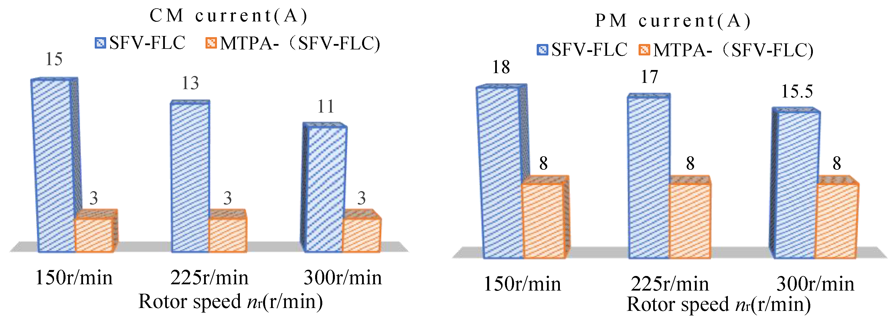
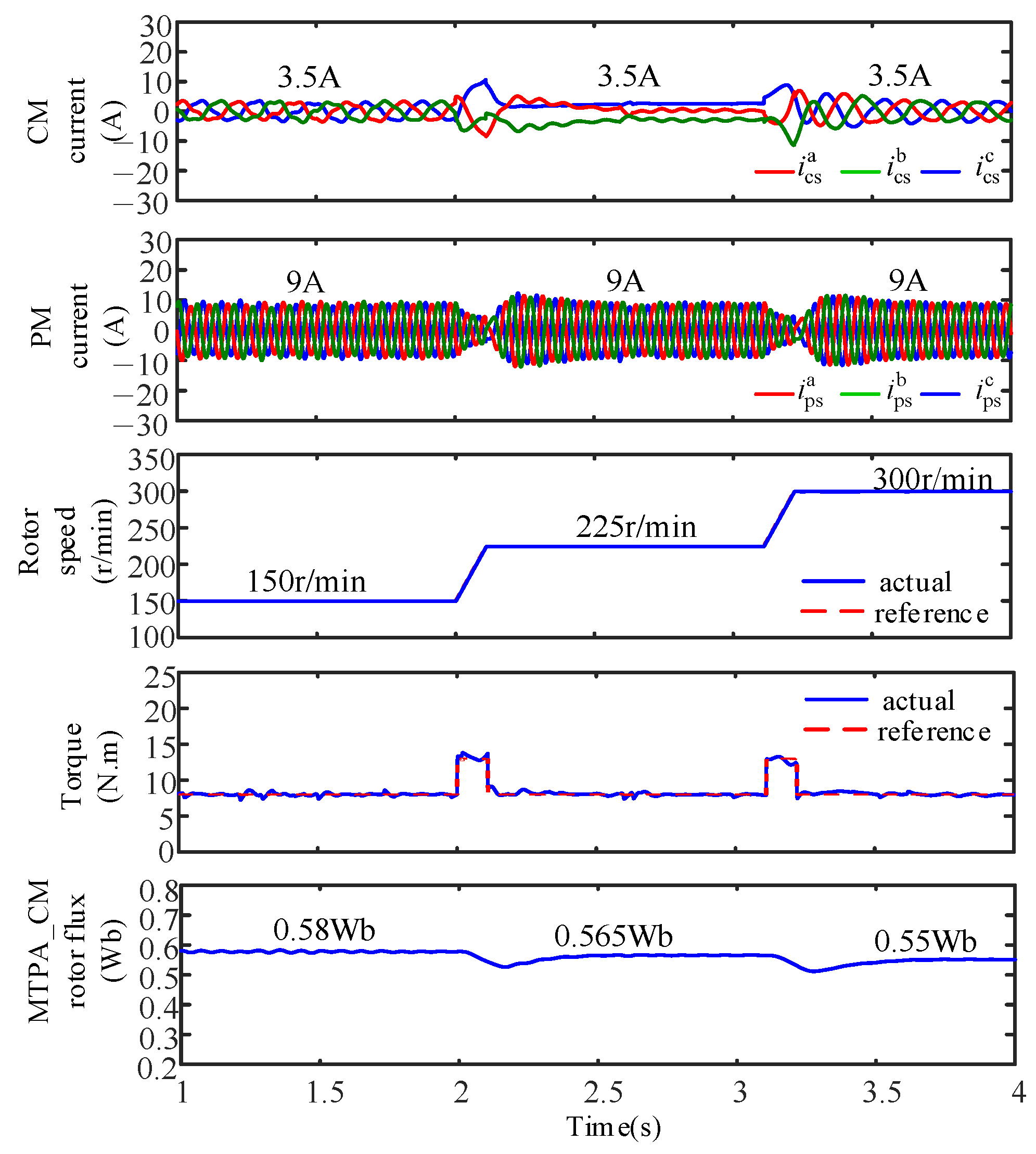
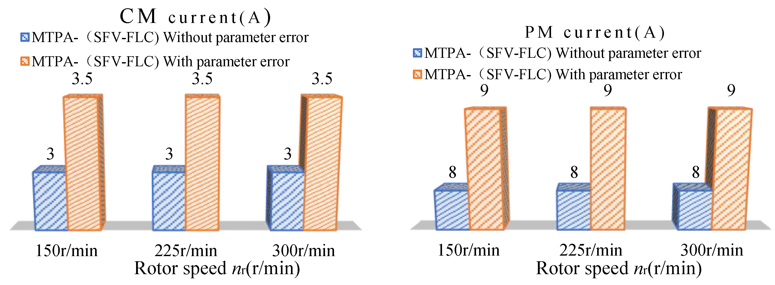
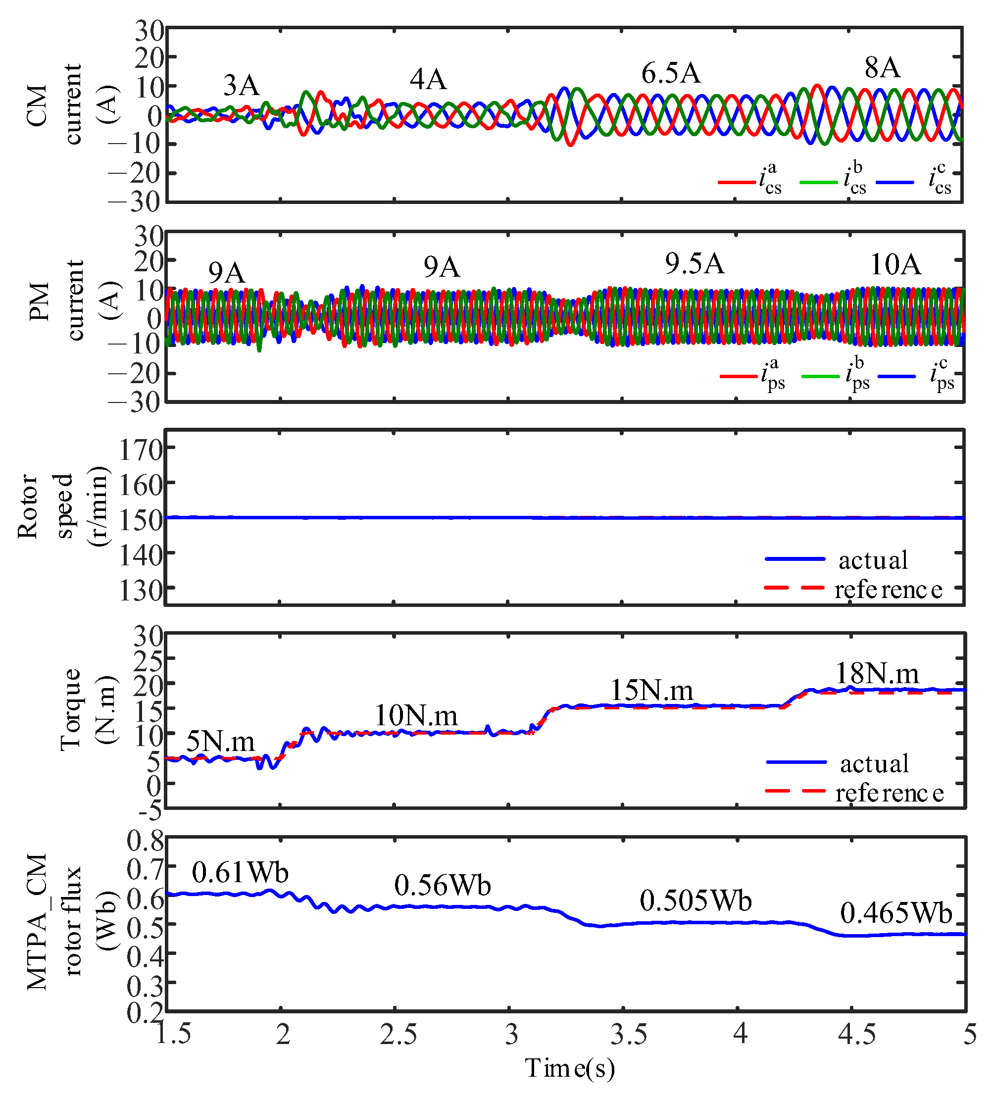
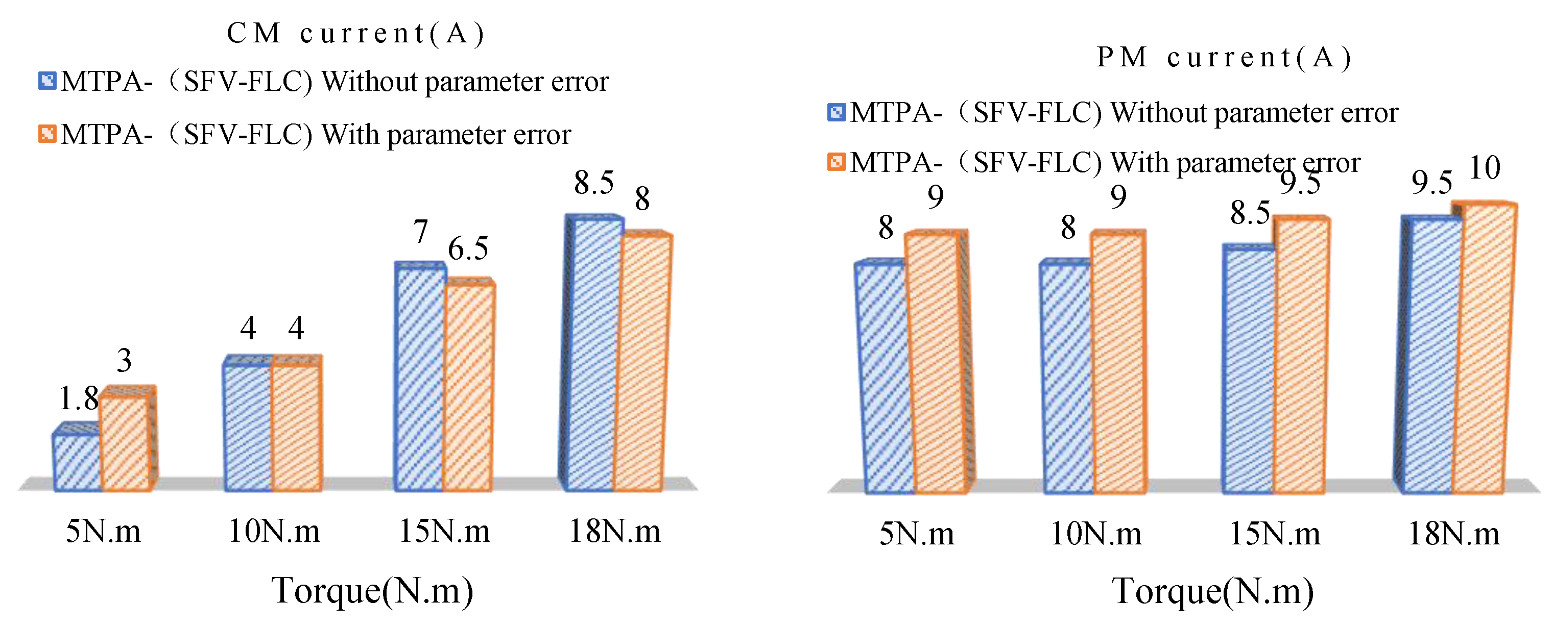
4.2. Verification of Robust Performance

To verify the robustness of the MTPA-(SFV-FLC), the rotor resistance rr in the MTPA-(SFV-FLC) control algorithm is reduced by 20%, the CM lcs, lcm and lcr, and the PM lps, lpm and lpr are increased by 20%, and the other conditions remain the same. When the speed varies, the simulation experiment results are depicted in Figure 11. Figure 12 shows the comparison data of the simulation experiment of the MTPA-(SFV-FLC) control algorithm with and without the parameter deviation. When the Torque varies, the simulation experiment results are depicted in Figure 13. Figure 14 shows the comparison data of the simulation experiment of the MTPA-(SFV-FLC) control algorithm with and without the parameter deviation.
It is indicated in Figure 11 that the CM rotor flux generated with parameter deviation by MTPA control is 0.01 Wb less than that without the parameter deviation, and the CM rotor flux generated by MTPA control decreases with the increase in the speed. This conclusion is confirmed by the theoretical analysis presented in Figure 6. As the speed increases from 150 r/min to 225 r/min and then to 300 r/min, the CM stator current is 3.5A, which is 0.5A larger than that without the parameter deviation. The PM stator current is 9A, which is 0.5A higher than the value when there is no parameter deviation. Although the stator currents of the two motors are slightly larger than the current without the parameter deviation, they are still much smaller than the stator current under SFV-FLC control. Table 4 shows the current comparison between the two control methods of the MTPA-(SFV-FLC) and (SFV-FLC) in the presence of the parameter deviations.
It is demonstrated in Figure 13 that the CM rotor flux generated with parameter deviation by MTPA control is 0.005 Wb less than that without the parameter deviation, and the CM rotor flux obtained by MTPA control decreases as the speed increases. This conclusion is confirmed by the theoretical analysis presented in Figure 5. When the torque changes from 5 Nm to 10 Nm, 15 Nm and 18 Nm, the CM stator current increases gradually from 3A to 4A, 6.5A and 8A, and the PM stator current gradually increases from 9A to 9A, 9.5A and 10A. The current difference is minuscule with the parameter deviation. From the results, we observed that when the motor is running with a light load, the stator current under MTPA-(SFV-FLC) is much smaller than that under the SFV-FLC. These results verify the superiority of the MTPA-(SFV-FLC) control and further verify that the control system is robust. Table 5 shows the current comparison between the two control methods of the MTPA-(SFV-FLC) and (SFV-FLC) in the presence of parameter deviations.

5. Conclusions

The paper introduced an MTPA optimal control method for the BDFM. The primary contribution of the proposed method is its ability to address the issue of large stator currents of the PM and the CM using a traditional SFV-FLC under no-load and light-load conditions. In the MTPA-(SFV-FLC) control scheme, the inner loop consists of the SFV-FLC, which facilitates the decoupling of the BDFM system. By implementing the MTPA control as the outer loop, the amplitude of the stator current can be effectively minimized, leading to an improved power factor and greater system efficiency. The simulation results demonstrate the effectiveness of the proposed MTPA-(SFV-FLC) control approach and the robustness of the control performance in the presence of errors affecting the controller and observer parameters.

Author Contributions

Conceptualization, C.X. and N.W.; methodology, C.X. and N.W.; software, C.X. and N.W.; validation, C.X. and N.W.; formal analysis, C.X. and N.W.; investigation, C.X.; resources, C.X.; data curation, C.X.; writing—original draft preparation, C.X. and N.W.; writing—review and editing, C.X. and N.W.; visualization, C.X. and N.W.; supervision, C.X.; project administration, C.X.; funding acquisition, C.X. All authors have read and agreed to the published version of the manuscript.

Funding

This research received no external funding.

Data Availability Statement

All the data are shown in the tables and figures of this paper.

Conflicts of Interest

The authors declare no conflict of interest.

References

  1. Sadeghi, R.; Madani, S.M.; Ataei, M.; Agha Kashkooli, M.R.; Ademi, S. Super-Twisting Sliding Mode Direct Power Control of a Brushless Doubly Fed Induction Generator. IEEE Trans. Ind. Electron. 2018, 65, 9147–9156. [Google Scholar] [CrossRef]
  2. Wei, X.; Cheng, M.; Zhu, J.; Yang, H.; Luo, R. Finite-Set Model Predictive Power Control of Brushless Doubly Fed Twin Stator Induction Generator. IEEE Trans. Power Electron. 2019, 34, 2300–2311. [Google Scholar] [CrossRef]
  3. Xu, L.; Cheng, M.; Wei, X.; Yan, X.; Zeng, Y. Dual Synchronous Rotating Frame Current Control of Brushless Doubly Fed Induction Generator Under Unbalanced Network. IEEE Trans. Power Electron. 2021, 36, 6712–6724. [Google Scholar] [CrossRef]
  4. Chen, H.; Jiang, B.; Ding, S.X.; Huang, B. Data-Driven Fault Diagnosis for Traction Systems in High-Speed Trains: A Survey, Challenges, and Perspectives. IEEE Trans. Intell. Transp. Syst. 2022, 23, 1700–1716. [Google Scholar] [CrossRef]
  5. Li, Y.; Chen, H.; Lu, N.; Jiang, B.; Zio, E. Data-Driven Optimal Test Selection Design for Fault Detection and Isolation Based on CCVKL Method and PSO. IEEE Trans. Instrum. Meas. 2022, 71, 3512310. [Google Scholar] [CrossRef]
  6. Bing, L.; Shi, L.; Teng, L.; Jia, Z. Duty Ratio Modulation Direct Torque Control of Brushless Doubly-Fed Machines. Automatika 2017, 58, 479–486. [Google Scholar] [CrossRef] [Green Version]
  7. Xia, C.; Hou, X. Study on the Static Load Capacity and Synthetic Vector Direct Torque Control of Brushless Doubly Fed Machines. Energies 2016, 9, 966. [Google Scholar] [CrossRef] [Green Version]
  8. Wang, Z.; Yang, M.Y. Vector Control Study for Cascade Brushless Doubly-Fed Machine. Adv. Mater. Res. 2012, 433–440, 7247–7252. [Google Scholar] [CrossRef]
  9. Shao, S.; Abdi, E.; Barati, F.; McMahon, R. Stator-Flux-Oriented Vector Control for Brushless Doubly Fed Induction Generator. IEEE Trans. Ind. Electron. 2009, 56, 4220–4228. [Google Scholar] [CrossRef]
  10. Zhang, G.; Yang, J.; Sun, Y.; Su, M.; Tang, W.; Zhu, Q.; Wang, H. A Robust Control Scheme Based on ISMC for the Brushless Doubly Fed Induction Machine. IEEE Trans. Power Electron. 2018, 33, 3129–3140. [Google Scholar] [CrossRef]
  11. Hopfensperger, B.; Atkinson, D.J.; Lakin, R.A. Stator Flux Oriented Control of a Cascaded Doubly-Fed Induction Machine. IEE Proc.—Electr. Power Appl. 1999, 146, 597. [Google Scholar] [CrossRef] [Green Version]
  12. Li, Y.; Xu, S.; Chen, H.; Jia, L.; Ma, K. A General Degradation Process of Useful Life Analysis Under Unreliable Signals for Accelerated Degradation Testing. IEEE Trans. Ind. Inform. 2022, 1–9. [Google Scholar] [CrossRef]
  13. Wang, N.N. Performance Analysis of Vector Control of Brushless Doubly-Fed Machine in Double Synchronous Reference Frame. In Proceedings of the 2022 25th International Conference on Electrical Machines and Systems (ICEMS), Chiang Mai, Thailand, 29 November–2 December 2022. [Google Scholar] [CrossRef]
  14. Xia, C.; Guo, H. Feedback Linearization Control Approach for Brushless Doubly-Fed Machine. Int. J. Precis. Eng. Manuf. 2015, 16, 1699–1709. [Google Scholar] [CrossRef]
  15. Wei, X.; Cheng, M.; Wang, W.; Han, P.; Luo, R. Direct Voltage Control of Dual-Stator Brushless Doubly Fed Induction Generator for Stand-Alone Wind Energy Conversion Systems. IEEE Trans. Magn. 2016, 52, 1–4. [Google Scholar] [CrossRef]
  16. Sun, T.; Long, L.; Yang, R.; Li, K.; Liang, J. Extended Virtual Signal Injection Control for MTPA Operation of IPMSM Drives with Online Derivative Term Estimation. IEEE Trans. Power Electron. 2021, 36, 10602–10611. [Google Scholar] [CrossRef]
  17. Khazaee, A.; Zarchi, H.A.; Markadeh, G.A.; Mosaddegh Hesar, H. MTPA Strategy for Direct Torque Control of Brushless DC Motor Drive. IEEE Trans. Ind. Electron. 2021, 68, 6692–6700. [Google Scholar] [CrossRef]
  18. Chen, H.; Liu, Z.; Alippi, C.; Huang, B.; Liu, D. Explainable Intelligent Fault Diagnosis for Nonlinear Dynamic Systems: From Unsupervised to Supervised Learning. IEEE Trans. Neural Netw. Learn. Syst. 2022, 1–14. [Google Scholar] [CrossRef] [PubMed]
  19. Li, Y.; Wang, X.; Lu, N.; Jiang, B. Conditional Joint Distribution-Based Test Selection for Fault Detection and Isolation. IEEE Trans. Cybern. 2022, 52, 13168–13180. [Google Scholar] [CrossRef] [PubMed]
  20. Shi, J.N.; Xia, C.Y. Feedback Linearization and Maximum Torque per Ampere Control Methods of Cup Rotor Permanent-Magnet Doubly Fed Machine. Energies 2021, 14, 6402. [Google Scholar] [CrossRef]
  21. Lee, K.; Han, Y. Reactive-Power-Based Robust MTPA Control for v/f Scalar-Controlled Induction Motor Drives. IEEE Trans. Ind. Electron. 2022, 69, 169–178. [Google Scholar] [CrossRef]
  22. Mosaddegh Hesar, H.; Abootorabi Zarchi, H.; Arab Markadeh, G. Online MTPTA and MTPIA Control of Brushless Doubly Fed Induction Motor Drives. IEEE Trans. Power Electron. 2021, 36, 691–701. [Google Scholar] [CrossRef]
  23. Ahmadian, M.; Jandaghi, B.; Oraee, H. Maximun Torque per Ampere Operation of Brushless Doubly Fed Induction Machines. Renew. Energy Power Qual. J. 2011, 1, 981–985. [Google Scholar] [CrossRef]
  24. Chen, H.; Li, L.; Shang, C.; Huang, B. Fault Detection for Nonlinear Dynamic Systems with Consideration of Modeling Errors: A Data-Driven Approach. IEEE Trans. Cybern. 2022, 1–11. [Google Scholar] [CrossRef] [PubMed]
  25. Xia, C.; Wang, N. Research and Analysis of the Characteristics of the Brushless Doubly-Fed Machine with High-Performance Decoupling Control. Machines 2023, 11, 313. [Google Scholar] [CrossRef]
  26. Li, Y.; Lu, N.; Shi, J.; Jiang, B. A Quantitative Causal Diagram Based Optimal Sensor Allocation Strategy Considering the Propagation of Fault Risk. J. Frankl. Inst. 2021, 358, 1021–1043. [Google Scholar] [CrossRef]
Figure 1. Structure diagram of BDFM [25].
Machines 11 00422 g001
Figure 2. MTPA online computing block diagram.
Machines 11 00422 g002
Figure 3. MTPA-(SFV-FLC) optimized control block diagram.
Machines 11 00422 g003
Figure 4. Calculation of ψ cr _ MTPA when the speed and torque vary.
Machines 11 00422 g004
Figure 5. ψ cr _ MTPA is computed when the torque changes.
Machines 11 00422 g005
Figure 6. ψ cr _ MTPA is computed when the speed changes.
Machines 11 00422 g006
Figure 7. Simulation experiment results when the speed changes. (a) SFV-FLC control method; (b) MTPA-(SFV-FLC) control method.
Machines 11 00422 g007aMachines 11 00422 g007b
Figure 8. Simulation data when the load torque is constant and the speed changes.
Machines 11 00422 g008
Figure 9. Simulation experiment results when the torque changes. (a) SFV-FLC control method; (b) MTPA-(SFV-FLC) control method.
Machines 11 00422 g009aMachines 11 00422 g009b
Figure 10. Simulation experiment data when the torque changes.
Machines 11 00422 g010
Figure 11. When the speed varies, the simulation experiment verifies the MTPA-(SFV-FLC)’s robustness.
Machines 11 00422 g011
Figure 12. The comparison data of the simulation experiment of the MTPA-(SFV-FLC) control algorithm with and without parameter deviation at different speeds.
Machines 11 00422 g012
Figure 13. When the torque varies, the simulation experiment verifies the MTPA-(SFV-FLC)’s robustness.
Machines 11 00422 g013
Figure 14. The comparison data of the simulation experiment of the MTPA-(SFV-FLC) control algorithm with and without parameter deviation at different torques.
Machines 11 00422 g014
Table 1. BDFM parameters [25].
ParameterValueParameterValue
P (kW)8ups (V/Hz)220/50
TN/(N·m)50rps/rcs (Ω)0.813/0.533
pp1rpr/rcr (Ω)0.6/0.493
pc3lps/lcs (H)0.372/0.0649
nr (r/min)1500lpm/lcm (H)0.367/0.0636
Table 2. Current comparison between the two control methods of MTPA-(SFV-FLC) and (SFV-FLC) when the speed changes.
nr (r/min) Δ i c s a b c % Δ i p s a b c %
150−80%−56%
225−76%−53%
300−72%−48.3%
where Δ i cs abc % = i c s _ MTPA - ( S F C - F L C ) a b c     i c s _ SFC - F L C a b c i c s _ SFC - F L C a b c Δ i p s a b c % = i ps _ MTPA - ( S F C - F L C ) a b c     i ps _ SFC - F L C a b c i ps _ SFC - F L C a b c .
Table 3. Current comparison between two control methods of MTPA-(SFV-FLC) and (SFV-FLC) when the torque changes.
Te (N.m) Δ i c s a b c % Δ i p s a b c %
5−89.4%−60%
10−71%−53%
15−36.3%−35%
18−6%−9%
Table 4. When there is a deviation in the parameters, the current comparison of the two control methods of MTPA-(SFV-FLC) and (SFV-FLC) at different speeds.
nr (r/min) Δ i c s a b c % Δ i p s a b c %
150−76%−50%
225−73%−47%
300−68%−42%
where
Δ i c s a b c % = i c s _ MTPA - ( S F C - F L C ) w i t h   p a r a m e t e r   e r r o r a b c i c s _ SFC - F L C a b c i c s _ SFC - F L C a b c
Δ i p s a b c % = i ps _ MTPA - ( S F C - F L C ) with   p a r a m e t e r   e r r o r a b c i ps _ SFC - F L C a b c i p s _ S F C - F L C a b c
Table 5. When there is a deviation in the parameters, the current comparison of the two control methods of MTPA-(SFV-FLC) and (SFV-FLC) at different torques.
Te (N.m) Δ i c s a b c % Δ i p s a b c %
5−82.3%−55%
10−71%−47%
15−41%−27%
18−8%−5%
Disclaimer/Publisher’s Note: The statements, opinions and data contained in all publications are solely those of the individual author(s) and contributor(s) and not of MDPI and/or the editor(s). MDPI and/or the editor(s) disclaim responsibility for any injury to people or property resulting from any ideas, methods, instructions or products referred to in the content.

