
Wear Parameter Diagnostics of Industrial Milling Machine with Support Vector Regression


Department of Mechatronics, Automation Technology and Mechanical Engineering, Tampere University, Korkeakoulunkatu 7, 33720 Tampere, Finland
*
Author to whom correspondence should be addressed.
Machines 2023, 11(3), 395; https://doi.org/10.3390/machines11030395
Submission received: 6 March 2023
/
Revised: 14 March 2023
/
Accepted: 16 March 2023
/
Published: 17 March 2023
(This article belongs to the Section Advanced Manufacturing)
Abstract
:Modern industrial machine applications often contain data collection functions through automation systems or external sensors. Yet, while the different data collection mechanisms might be effortless to construct, it is advised to have a well-balanced consideration of the possible data inputs based on the machine characteristics, usage, and operational environment. Prior consideration of the collected data parameters reduces the risk of excessive data, yet another challenge remains to distinguish meaningful features significant for the purpose. This research illustrates a peripheral milling machine data collection and data pre-processing approach to diagnose significant machine parameters relevant to milling blade wear. The experiences gained from this research encourage conducting pre-categorisation of data significant for the purpose, those being manual setup data, programmable logic controller (PLC) automation system data, calculated parameters, and measured parameters under this study. Further, the results from the raw data pre-processing phase performed with Pearson Correlation Coefficient and permutation feature importance methods indicate that the most dominant correlation to recognised wear characteristics in the case machine context is perceived with vibration excitation monitoring. The root mean square (RMS) vibration signal is further predicted by using the support vector regression (SVR) algorithm to test the SVR’s overall suitability for the asset’s health index (HI) approximation. It was found that the SVR algorithm has sufficient data parameter behaviour forecast capabilities to be used in the peripheral milling machine prognostic process and its development. The SVR with Gaussian radial basis function (RBF) kernel receives the highest scoring metrics; therefore, outperforming the linear and polynomial kernels compared as part of the study.
1. Introduction
Advanced sensor systems and smart devices are widely developing and simultaneously enabling real-time monitoring of asset behaviour through cloud services. From the industrial business perspective, continuous asset monitoring and online data collection not only create condition-based maintenance (CBM) possibilities, but also enable a more holistic understanding of machine behaviour through machine learning (ML) technologies. This understanding can be further capacitated for researching new business opportunities, such as the pay-per-x (PPX) business models [1], where the ownership of an asset is partly or fully retained by the machine builder. In PPX business making, the customer payment is at least partly connected to the output or outcome created by using the asset. Further, the timely synchronous situational awareness of the machine’s current condition and condition prognostics not only diversifies the original equipment manufacturer (OEM) business offering from traditional investment business making to pay-per-outcome/output-related business making [2], but the technological advancements may also offer enriched data of the process or factory level bottlenecks and improvement areas for the end-user. Overall, the examination of various types of structured or unstructured data correlations within the company’s assets can ultimately result in competitive advances against competitors, increased revenue streams, and enable efficient decision-making [3].
Establishing a multidimensional data collection system, including data transfer capabilities, is rather effortless in present times with embedded data system capabilities and seamless integration of external sensors [4]. Despite the easiness of the data collection, many small- and medium-sized companies are distrustful of their internal capabilities to utilise the data, mainly due to a lack of knowledge in data analyst skills. Additionally, at the time of initiating machine data exploration discussions inside the company, the diversity of available data sources as well as machine learning tools might be cumbersome to the companies to know where to start and how to formulate the data into knowledge useful for their business. To overcome this challenge, a seamless collaboration between domain knowledge holders and data analysts needs to be established to mutually understand the machine’s operational characteristics, as well as to understand the purpose of use for the collected data. Additionally, at the beginning of the process, more simplified data-based machine learning models are recommended, as they include easier implementation [5]. The gradually developing work process also creates more synergies between the parties by awarding quicker results and giving a partial understanding of the phenomena already at the beginning of the process, although using more complex models might offer higher predictive power [6], resulting in more accurate results.
In an industrial context, the collection of machine-related data is often used to enhance a machine’s performance within its operation. Data collected are rarely used as such, but require pre-processing [7] as well as an understanding of the scale and meaning of parameters relevant to the machine’s operational condition evaluation. In the milling machine context, one of the key elements is to understand the milling tool blade wear behaviour in correlation to its usage. It is essential to comprehend the data and recognize tool wear indicators in order to differentiate linear wear to enable timely and cost-effective blade changes. Furthermore, this data is also exploitable to improve machining precision and part quality [8]. Data sources applicable for tool condition monitoring and remaining useful life (RUL) approximation are generally recognised in earlier research to contain cutting force [9,10,11] exploration, milling cutter torque [10] measurements, tool temperature monitoring [12,13], and acoustic emission [11,14] as machine learning model input parameters. In addition, the collection of a vibration signal parameter is one of the most used measurements for recognising wear [9,10,15,16] behaviour from the collected data, especially in applications where continuous processing of real-time data is needed [17].
Different regression algorithms are commonly used in prediction-making by evaluating the correlation between dependent and independent variables. A data-driven random forest (RF) algorithm is used for wear prediction in comparison with artificial neural networks (ANN), and support vector regression (SVR) with kernel comparison of Gaussian radial basis function (RBF) and sigmoid kernel [18]. While the result from RF is found to have a good fit in prediction making, the time needed for training is greater than with the other algorithms, and RF model applicability to real-time applications is not supported by the research results. Another study illustrated machine health degradation monitoring from a vibrational raw signal by a generalised multiclass support vector machine (GenSVM) [19]. The method achieved superior results for the model in comparison to the standard support vector machine (SVM) algorithm, least squares support vector machines (LSSVM), k-nearest neighbour (KNN), back propagation neural network (BPNN), and adaptive network-based fuzzy inference system (ANFIS). The presented results give a good background for the SVM model’s capability to be tailored and used in predicting selected dependent variables with other data received from machine operation. However, an algorithm called support vector regression (SVR) algorithm is considered a more versatile version of SVM due to its extended hyperparameter settings. Benkedjouh et al. [20] used SVR for tool wear assessment and RUL prediction by using cutting force, vibration, and acoustic emission signals. The SVR generalisation capabilities for unseen data are recognised in [21], and extensive studies for SVR prediction accuracy in [18,22,23]. The relationship between the SVR’s independent and dependent variables is depicted in detail in [21,24]. To summarise, the SVR has an additional tuneable parameter ε (epsilon) to fit the hyperplane into the case dataset. Epsilon is a hyperparameter that controls the amount of allowable error in the model. The regularisation parameter (C) is used in the SVM tuning and it controls the trade-off between maximising the margin and minimising the training error [25,26]. However, it is recognised that the SVR algorithm’s well-known challenge is to comply with large datasets [27] and noisy data containing outliers [28]. This restricts the implementation of the algorithm in real-life applications where long-term prognostication with changing input parameters is naturally present.
This research illustrates the process of establishing a data connection from industrial peripheral milling machine operation and extracting meaningful data characteristics correlating with machine wear behaviour. In addition, the SVR algorithm is tested to receive a contextual understanding of the machine learning methods suitable for predicting dependent variable behaviour. The results of this study give valuable information for industrial companies to start or to continue developing their data collection systems and analysis methods suitable for their portfolio.
2. Methods: Peripheral Milling Machine Architecture and Data Acquisition
The technological viewpoint of this study is to recognise and implement PPX-enabling technologies and methods for industrial companies. In this research, the case machine was a peripheral milling machine operating in the marine industry. The milling process prepared welding contacts for support beams used in vessel structural construction. Operational environmental conditions for the milling process were controlled: the machine operated indoors under normal operating conditions at an approximate temperature of 20 degrees Celsius, with no exposure to external stresses such as temperature variations or excessive impurities. Hence, the data collected and analysed in this study rely upon the manufacturing process schedules and process parameters determined by the end user. Due to this, the milling process remained uncontrolled during the whole duration of the data collection, resulting in uncertainty challenges in comparison with supervised research conditions in a laboratory environment. However, a remote data connection was established, thus granting comprehensive access to the collected data.
2.1. Operation and the Architecture of the Milling Machine
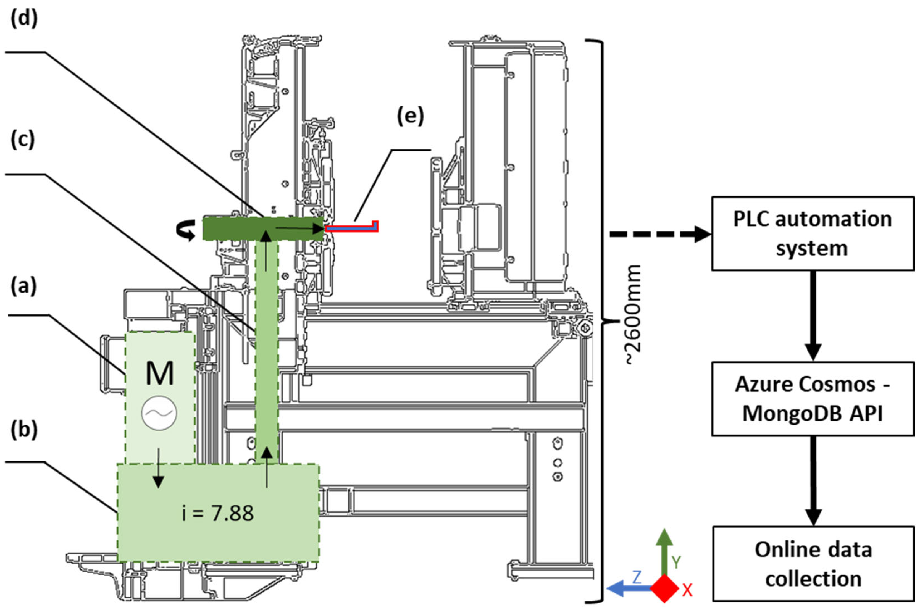
An internal automation system steered the peripheral milling machine controls and adjustments. A PLC system collected data from connected inputs [29] such as sensor data or operator commands [30], which were further combined in a collectable data format. In addition to the milled profile data, operation-related parameters were collected by the PLC, including the main powerline components, and milling position-related data. Figure 1 illustrates the main components of the milling machine in power direction sequence a–d, being an alternating current electric motor, a gear unit (with a 7.88:1 gear ratio), a shaft, and a spindle with the cutting blades, respectively. The L-shape profile is illustratively positioned against the spindle in Figure 1e, having material supply to down-feed milling from the x-axis direction. The force direction from the AC motor to the spindle and the spindle rotation direction is depicted by arrows in the figure. Other structural components such as conveyer line components or servomotors are not separately annotated due to their recognised irrelevance in researching blade wear under normal operation. The data flow from the machine PLC to the internet data collection interface was created through Azure Cosmos MongoDB application programming interface (API).
2.2. Data Acquisition
The data flow from the PLC was built through the Azure Cosmos MongoDB API. The API interface enabled online data access to the collected data by a third party [31]. The data transfer function was enabled through a Spyder scientific programming environment, which also enabled Python programming language utilisation including data feature dimensionality reduction and statistical regression models [32,33,34]. The raw data collected included 5,141,641 data rows, each containing data from 39 parameters.
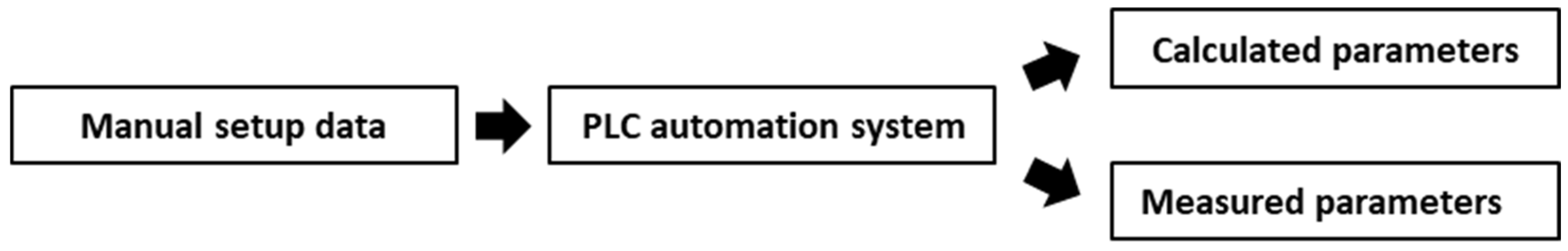
The data acquisition setup was established to contain collectable data from four categories: manual setup data, PLC automation system, calculated parameters, and measured parameters, with the number of collected parameters 7, 8, 18, and 6, respectively. The manufacturing sequence and data acquisition flow began with manual setup data input specified by the machine operator as illustrated in Figure 2. This manual input engaged predetermined machine configurations in the PLC automation system and activated the milling process. Some of the collected parameters were calculated based on the previous input, and the remainder by other measurements connected to the PLC.
The physical dimensions of the milled profiles varied depending on their use in the manufacturing process. The milled profile thickness varied between 5 and 30 mm, profile length in the range of 6000 to 23,800 mm, and profile height between 70 and 200 mm. The process operated in a semiautomatic manner, where the machine operator controlled the feed into the milling machine. Often, a certain type of profile was manufactured in larger batches instead of milling individual profiles. The manual setup data input was mandatory to specify the profile’s physical dimensions (height, length, and thickness), as well as the ‘Profile Type’ between I-beam or L-beam type presented in Table 1. The ‘Milling part ID’ refers to the individualised numbering of the profiles for quality tracking. To minimise unnecessary production downtime, two separate spindle tools were used and numbered in the production. Whilst spindle 1 was in operation, the cutting blades were changed to spindle 2 and vice versa. An individual spindle contained four rows of cutting blades: two rows had a 90°, and two rows 86° contact angle to the milled material, each row containing 18 cutting blades. The operator selected the spindle ‘Tool number’ and ‘Spindle position’ (blade row in use) that were currently in use.
Once the manual setup data was fed through the machine’s user interface, the PLC automation system selected the predetermined milling settings based on the given input and started indexing the process with a ‘Time stamp’. After receiving permission from the operator to start the process, the machine automatically collected the required profiles from the material depository and began production with the pre-set values for cutting speed, feed rate, mill depth, and frame position. The Boolean data (true/false) of the machine in active state and milling status were also recorded.
Various parameters were mathematically formed and collected to the central database located in local data storage, which was further connected online for remote data collection. The cutting speed ratio and feed rate ratio in Table 2 were calculated to monitor the difference between set and measured values. The ‘Number of tool rows used’ parameter was recorded to indicate possible simultaneous usage of blades with higher thickness (>19.1 mm) profiles, which was deemed usable when observing cumulative wear behaviour in the blades. The four tool rows were numbered from 0 to 3 (as indicated in Table 1, spindle position) to gain cumulated usage data on individual tool rows. The parameters milled meters and total milling time were calculated by utilising profile length, length of cut, feed rate, and spindle speed [35] input, the latter being calculated from the cutting speed. The row-specific Boolean type of true/false (T/F) information was further recorded to assist in the visual inspection of the data. The cumulative minimum, maximum, and average milled meters were obtained to gain an understanding of the differences between milling cycles and to work as a preliminary index parameter for the wear behaviour observation.
The measured operational parameters were mainly received through the machine’s embedded systems. The cutting speed, feed rate, AC motor torque, and time constraints (milling operations starting and ending time) were received directly through the automation system computer statistics. The collection of vibration signals was established through an external analogue vibration sensor attached in the radial direction relative to the spindle cutting blades. The raw vibration signal collection enabled vibration velocity root mean square (RMS) calculations from the time domain signal. The transformation of the raw data signal to velocity RMS values were preconfigured to the PLC system, leaving exploitation of the raw signal inaccessible for research purposes. Therefore, only the pre-decimated value of the vibration velocity RMS (mm/s) given by the PLC system was exploited in this research.
3. Data Pre-Processing and Feature Reduction Process
Multidimensional data collection enables versatile and wide-ranging investigation of data features and their correlation with each other. Often, the connection of different features meaningful for the purpose can be manually diagnosed by expert opinion or basic statistical analyst skills. However, data pre-processing tools such as Pearson Correlation Coefficient (PCC) and Permutation Feature Importance (PFI) become essential in the data pre-processing phase, especially when the amount of data becomes immense for manual analysis. PCC and PFI tools used in this research operated in an unsupervised manner to recognise the correlation of different data features that were relative to the milling tool blade wear. Additionally, the feature reduction process had an obvious positive influence on training and testing times for many of the regression algorithms [23].
3.1. Pearson Correlation Coefficient (PCC)
Pearson Correlation Coefficient (PCC) is a commonly used feature correlation indication tool that measures the linear correlation between the parameters [10]. The PCC assessment was performed on the complete dataset with the features presented in Table 1 and Table 2. These features illustrated all the data originally collected from the operator input and machine operation. Pearson correlation formula is exhibited in Equation (1), as presented in [10,36].
where is the identification number of a single data point, is the first individual data point, and denotes the corresponding arithmetic mean of the first sample. Following, the and are the corresponding samples of the comparable variable, in this case, the cumulative average value of milled meters. The linear correlation between and ranges between +1 and −1, where the (−) negative result indicates a negative correlation and (+) presents a positive correlation between the data points [37]. High feature correlation value varies significantly, some earlier research recognised high correlation values variating from 0.8 [19] to >0.98 [37].
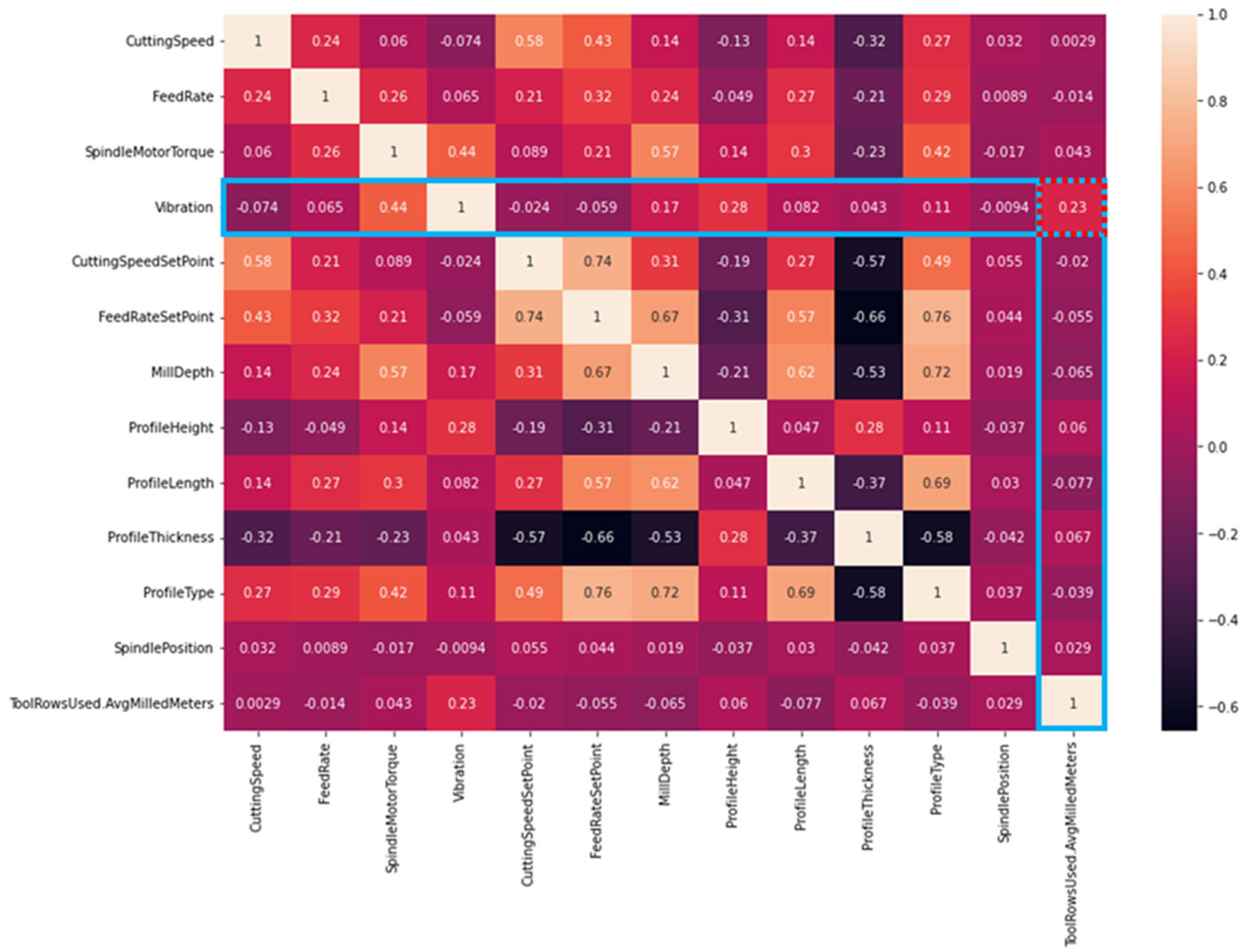
In this research, the PCC was iterated to scale down the number of features from the original 39 features to 13, where the features indicating a clear categorical negative correlation were removed. The numeric results of the finally selected 13 features and their correlations are combined in a heatmap format, as presented in Figure 3.
As a result, the PCC scores for high correlation remained lower, as presented in the earlier research. Despite the iterative feature reduction, the data remained rather high in dimensionality (13 features), which likely resulted in lower scoring in comparison with less complex correlation maps where more obvious connection features might exist. The top three features correlating with the ‘Vibration’ are: ‘SpindleMotorTorque’ (0.44), ‘ProfileHeight’ (0.28), and ‘ToolRowsUsed.AvgMilledMeters’ (0.23). The highest value, ‘SpindleMotorTorque’, is evident due to physical consequences in increasing/decreasing torque affecting the vibration amplitudes in the cutting phenomenon. The correlation in the ‘ProfileHeight’ and other cutting material size properties also remain positive (+) due to similar justification, where the material physical features affect operational cutting forces and vibration amplitudes. The highest correlation to the cumulative usage of the milling blades (‘ToolRowsUsed.AvgMilledMeters’) is with the ‘Vibration’ parameter highlighted in the figure, with a correlation value of 0.23.
3.2. Permutation Feature Importance (PFI)
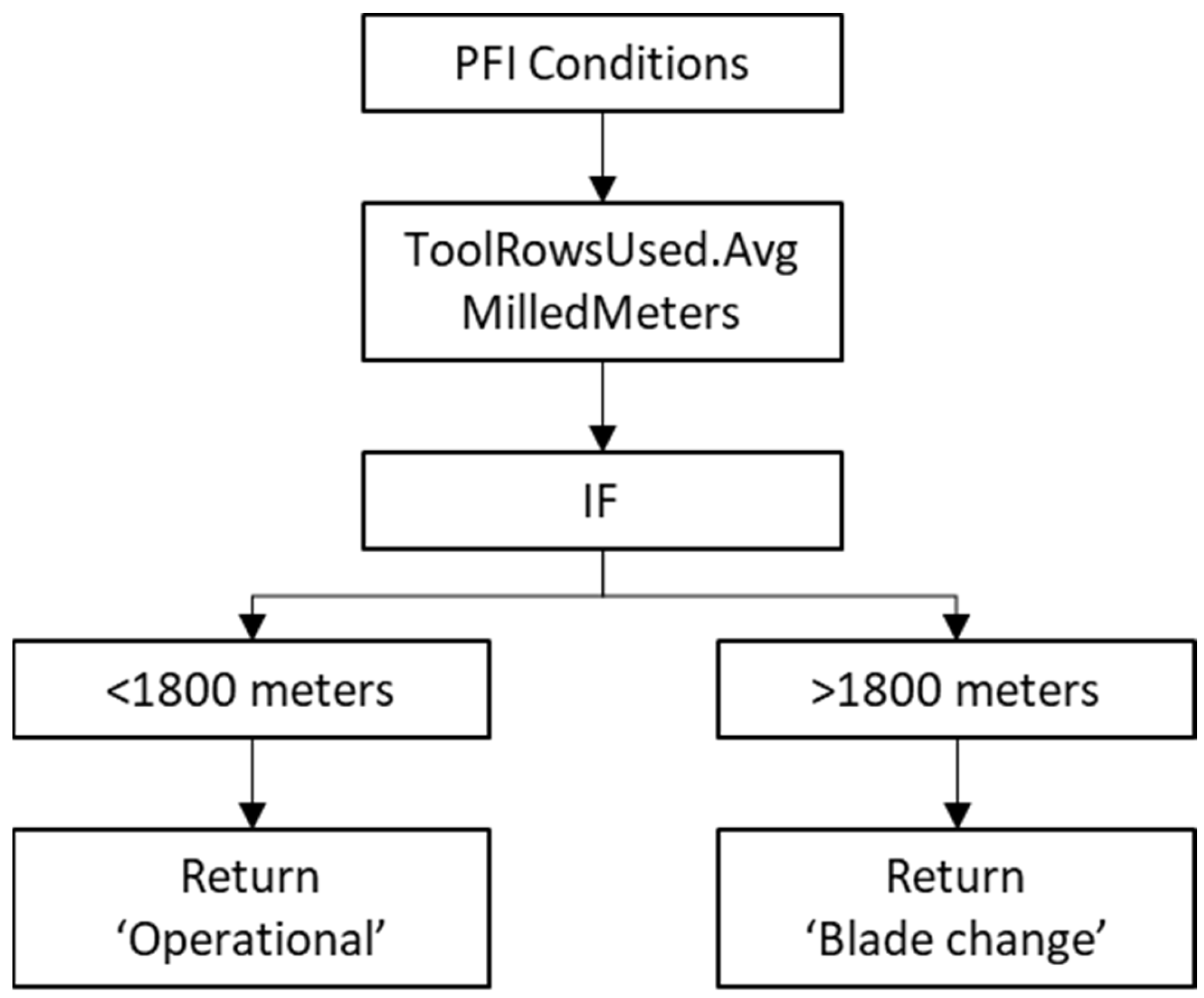
The number of originally collected parameters were scaled down by using the PCC in the previous section. In the permutation feature importance (PFI) phase, the length of the dataset was reduced to include two (2) full milling cycles (one containing approximately 2000 m of cumulative milling meters) to optimise the time needed for training the algorithm. The permutation feature importance method was conducted to address the order of the important factors in comparison to cumulative cutting meters (selected dependent variable). The PFI describes the connection between input features and the dependent variable and estimates how much each feature affects the performance of the model [38]. The variable selection was performed based on results indicated by the PCC analysis. The dependent variable was then compared with the other operational data collected from the actual machine operation to emphasise the feature significance in the calculation. The conditions for the permutation feature importance algorithm are depicted in Figure 4.
The categorisation limits of blade conditions were stated as follows: ‘Operational’ if the datapoint cumulative milling meter was less than 1800 m and ‘Blade change’ when the value exceeded 1800 m. The hypothesis of the linear blade condition was set based on expert opinion. The hypothesis of the estimated operational endurance of the cutting blades was considered without any anomalistic states. Hence, the health index (HI) categorisation was adjusted to the model as ‘Blade change’: 0, and ‘Operational’: 1, where the algorithm condition was forced to categorise the data between the states described above. Instead of a data shuffling method, the data column of ‘ToolRowsUsed.AvgMilledMeters’ was dropped out to receive the features the model considered most reliable.
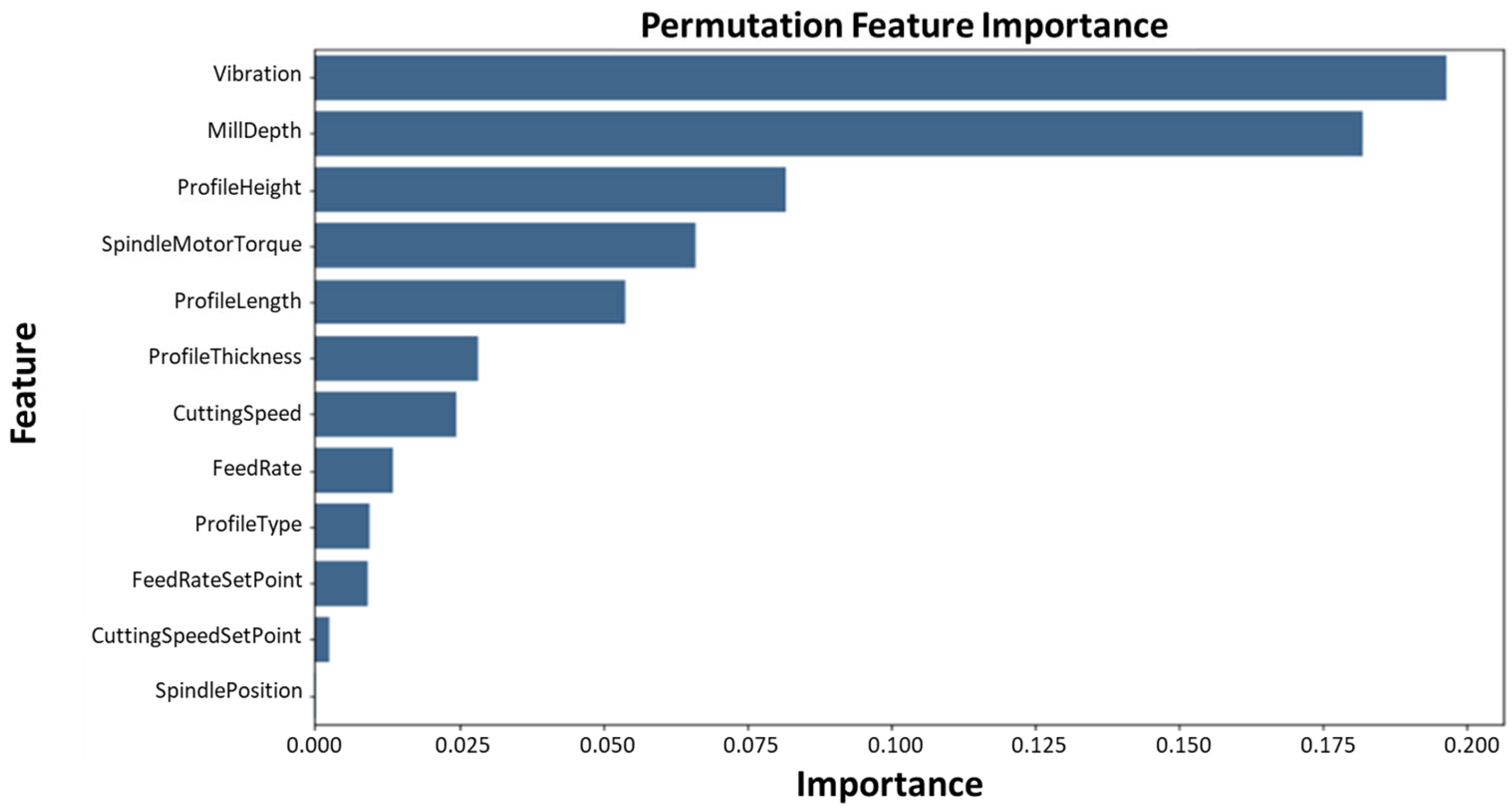
The area under the receiver operating characteristics (ROC) [39] curve (AUC) is broadly used to evaluate the performance for classification and diagnostic rules [40]. AUC is herein used to measure the performance of the classification between the given HI classes. The AUC result interpretation comparing the operational performance of regression models is depicted in [41]. A value of 1.0 is an immaculate test result, whereas results of <0.5 are insufficient and the model’s positive and negative objectives need to be redefined. Values of 0.9–0.99 are excellent test results, whereas 0.8–0.89 can be considered good, 0.7–0.79 as fair results, and 0.51–0.69 as poor test results [41]. In this study, the final AUC result of 0.923 was received with a random state = 10 setting. The results of the permutation feature importance are visualised in Figure 5.
Given the conditions determined in Figure 4, the permutation feature importance results in Figure 5 indicate that the ‘Vibration’ feature had the most significant correlation to ‘Operational’ and ‘Blade change’ conditions. Similarly with the PCC results, the PFI scoring levels remain low, yet illustrating the main feature of ‘Vibration’ being the dominant of the features in correlation to cumulative milling distance performed by the peripheral milling machine. The feature ‘MillDepth’ existed as a second important feature due to the variating milling recipes driven during the two datasets.
To conclude, the feature correlation methods of PCC and PFI gave a robust base for selecting the ‘Vibration’ feature to be dominant concerning the recognised linear wear behaviour occurring over accumulating milling time. The pipeline from the start point with the original dataset to the dominant feature selection is illustrated in Figure 6. The knowledge received from this process can be transferred back to the data collection setup, such as by increasing the number of vibration measurement sensors in different physical directions and/or frequency ranges to enable more comprehensive data and to receive a better understanding of the operation versus wear behaviour phenomenon.
4. Supervised Wear Feature Analysis with Support Vector Regression
In this work, the two SVR hyperparameters (ε and C) were adjusted to find the best fit for the model. The value of ε determined the width of the tube around the estimated function (hyperplane). The parameter C was a regularisation parameter to control the importance of the data points left outside the support vector boundaries and penalised data points containing errors greater than ε by a positive constant [26]. Points that fell inside this tube were justified as correct predictions and were not penalised by the SVR algorithm. The ‘Vibration’ parameter signal was used in the signal prediction as depicted in the earlier-presented dimensionality reduction results.
4.1. Kernel Classifier Selection
Obtaining appropriate hyperparameter settings is a common challenge in SVR implementation. However, defining an appropriate kernel function and hyperparameter settings is necessary to receive higher accuracy in the results [26]. The most used kernels include polynomial (POLY), Gaussian radial basis function (RBF), and sigmoid kernels, according to research made by [18]. In this research, the POLY and RBF kernels were adopted due to their better capability to accommodate nonlinear data. Additionally, the linear kernel was tested to prove the hypothesis of being less efficient on multidimensional data [42], resulting in a less accurate fit to the dependent variable data.
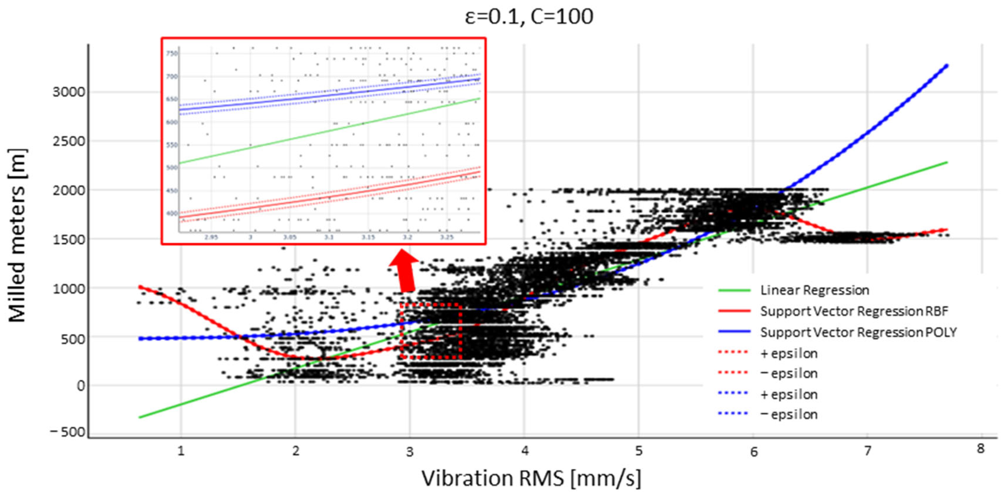
The hyperplane fitting is visually illustrated in Figure 7. The illustration presents one (1) peripheral milling machine operational cycle, where the operational milling distance was 2003.43 m. Upper (+) and lower (−) epsilon boundaries are illustrated with a dashed rectangle on top of the SVR-related hyperplanes in Figure 7, where the hyperplane fitting is performed with ε = 0.1, C = 100. The SVR hyperplane fitting towards the milling cycle data was also tested with several other manually selected hyperparameters; however, the ε = 0.1, C = 100 selection resulted in the most accurate hyperplane fitting.
The linear regression is presented in a green trend line in Figure 7 and Support Vector Regression with RBF is presented in the red trend line. The polynomial kernel POLY presented in the blue trend line showed no clear visual changes once the tuning parameters were changed. However, the quantitative error scoring of the training and test scores displayed in a squared correlation coefficient (R2), illustrated in Table 3, demonstrated more clearly the model’s ability to perform training and testing for the data compared with the visualised format in Figure 7. Quantitative comparison between multiple ε and C values resulted in the highest R2 train and score values with the ε = 0.1, C = 100 settings; therefore, the model scoring comparison between linear, polynomial, and RBF kernels were performed with the illustrated parameters for the SVR regression.
The scores in Table 3 demonstrate the inability of the linear kernel to fit the data properly, given the model R2 scoring both in the training and test phases between 0.646 and 0.649. The R2 scoring improved significantly with the SVR POLY (0.803–0.819) and received the highest score with SVR RBF (0.846–0.856). The mean absolute error (MAE) and mean squared error (MSE) [%] given by the RBF kernel were also at acceptable levels, being 0.0496 and 0.0046, respectively. The details of the model error scoring functions R2 and MSE are depicted in [25], and MAE in [43]. Overall, the SVR regression with RBF kernel selection outperformed the linear and polynomial equivalents in all the scoring metrics.
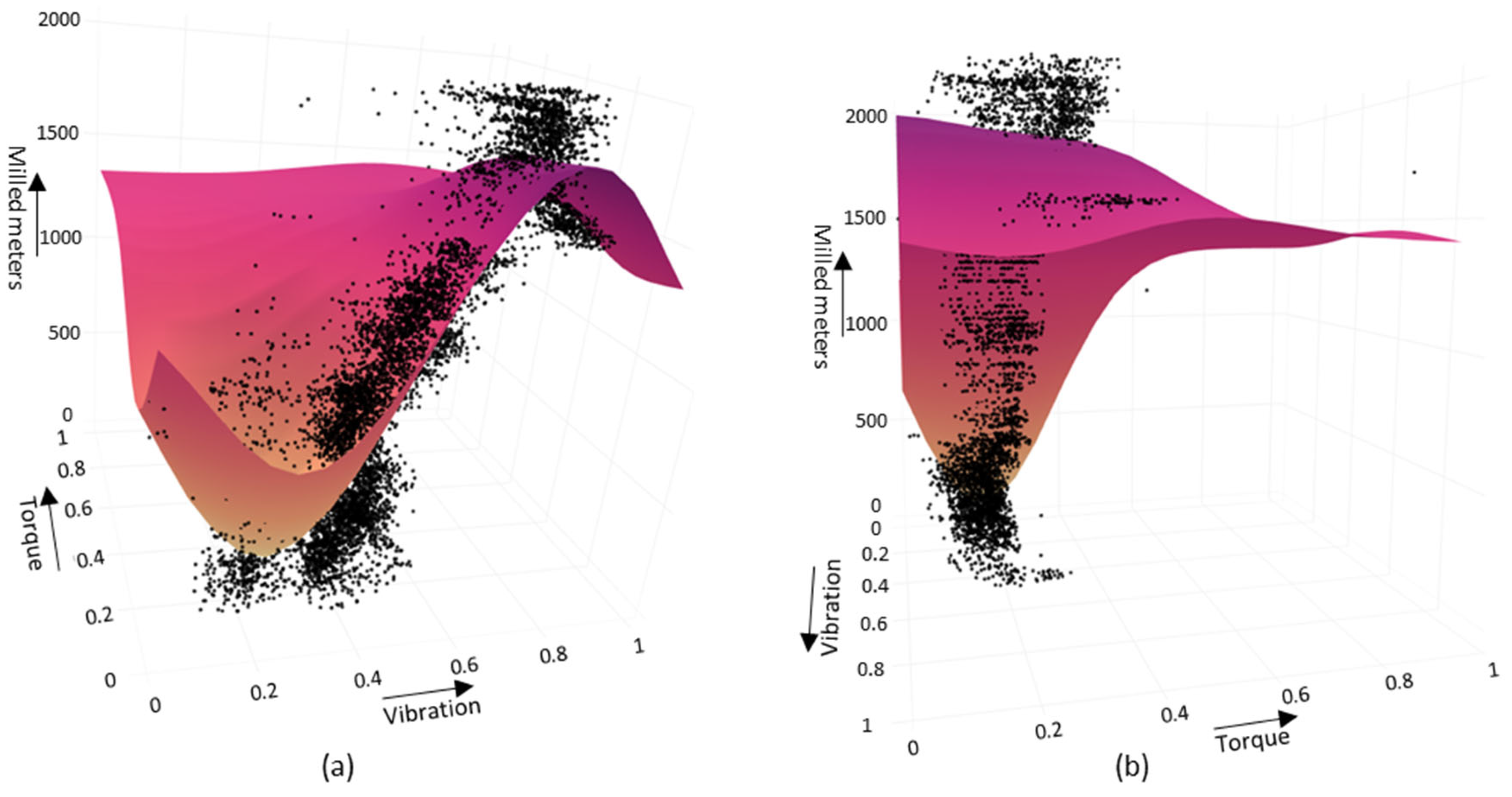
The 2D illustration and quantified values of the hyperplane fit based on the error scoring justify the SVR RBF being the most effective kernel for the purpose. To visualise the hyperplane fit in a higher dimensional format, an additional feature was added to establish a 3D figure. Some earlier research discovered that the wear symptoms in milling are visible by examining machine power consumption and related torque values [44,45]. The measured torque presents the cutting force affecting the cutting tool edges while in contact with the milled material due to its rotating motion [35]. Additionally, the results relative to the milling progress from both the PCC (dominant relative feature) and PFI (#4 dominancy) indicate torque parameters’ high correlation to vibration and the cumulative value of milled meters. Therefore, the torque effect is visualised as the third component in Figure 8.
The dataset was normalised with the MinMaxScaler function to rescale the targeted parameters ‘Vibration’, and ‘SpindleMotorTorque’ to ‘Vibration (scaled)’, and ‘SpindleMotorTorque (scaled)’ by using the scale of zero…one, respectively. The feature scaling operation normalised the value ranges of independent variables [46], allowing comparing feature values that normally operate on different value scales. Figure 8a illustrates a better viewpoint for the cumulative effect on ‘Vibration (scaled)’, and Figure 8b for the ‘SpindleMotorTorque (scaled). The visual observation of the feature space in Figure 8a illustrates the clear connection between the cumulative milling meters and increased vibration behaviour. The operational milling recipe changes during the milling cycle falsified the curvature of the hyperplane to point downwards towards the end of the milling cycle. Figure 8b illustrates that the torque dimension was moderately spreading towards the end of the milling cycle (milled meters). This observation supports the PCC and PFI results, indicating that the parameter affects the correlation between torque value and the cumulative milling process.
4.2. Vibration Analysis with the SVR (RBF)
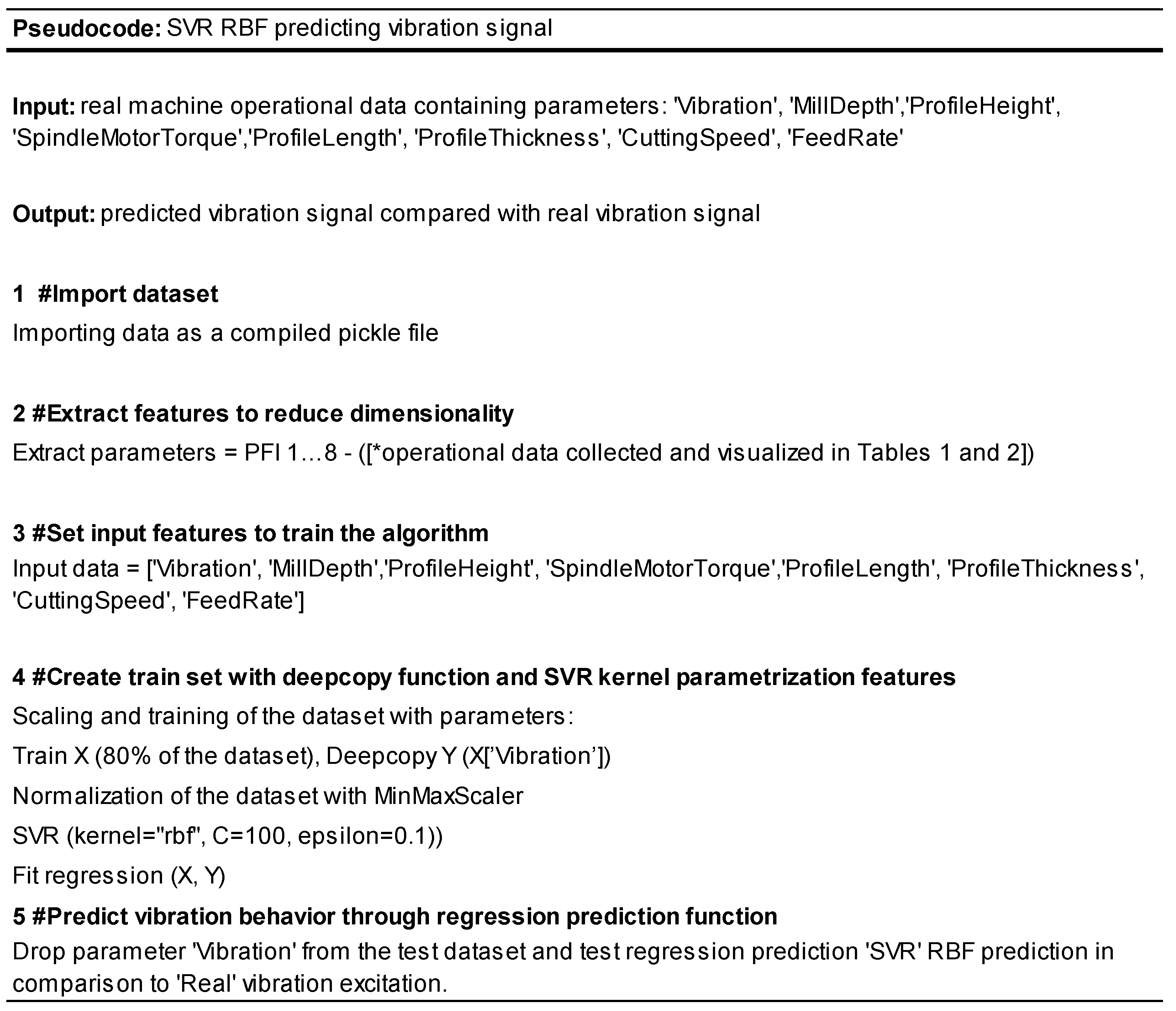
In this section, the SVR is utilised to predict the vibration signal based on the selected inputs. The kernel parameters used (RBF; ε = 0.1, C = 100) were justified in the earlier sections of this research. The presented pseudocode in Figure 9 was initiated to describe the main principles of the SVR algorithm. The main steps in the code are numbered between one and five, starting from the dataset import function, with the eight most important features selected from the PFI phase. After importing the complete dataset, the selected features were extracted from the raw data in step two and set as algorithm training features in step three. Then, the pseudocode description stated to split the given data into train and test splits and to rescale all the feature input values between zero and one, as determined in step four. The SVR algorithm predicted the dependent variable by identifying a hyperplane in a high-dimensional feature space that had the maximum margin of separation from the data classes [23]. The hyperplane was chosen such that it passed through as many data points as possible, and the distance between the hyperplane and the closest data points, called support vectors, was minimised [27]. In SVR, the correlation between the independent and dependent variables is described by a deterministic function in [21,24,27]:
where the transposed parameter weight vector w and bias b are unknown coefficients. w is a weight vector in that controls the importance of each feature in the model. The phi ϕ(x) represents a dot product function from input space to feature space [24]. y is the predicted output value for input x. The used Gaussian radial basis function (RBF) kernel enables nonlinear regression fit to the data. In the last stage (No. five) of the pseudocode, the dependent variable ‘Vibration’ is removed and exposed to the test part of the dataset to compare the regression model fit compared with the real vibration trend behaviour. The training set size corresponds to 80% of the total size of the dataset.
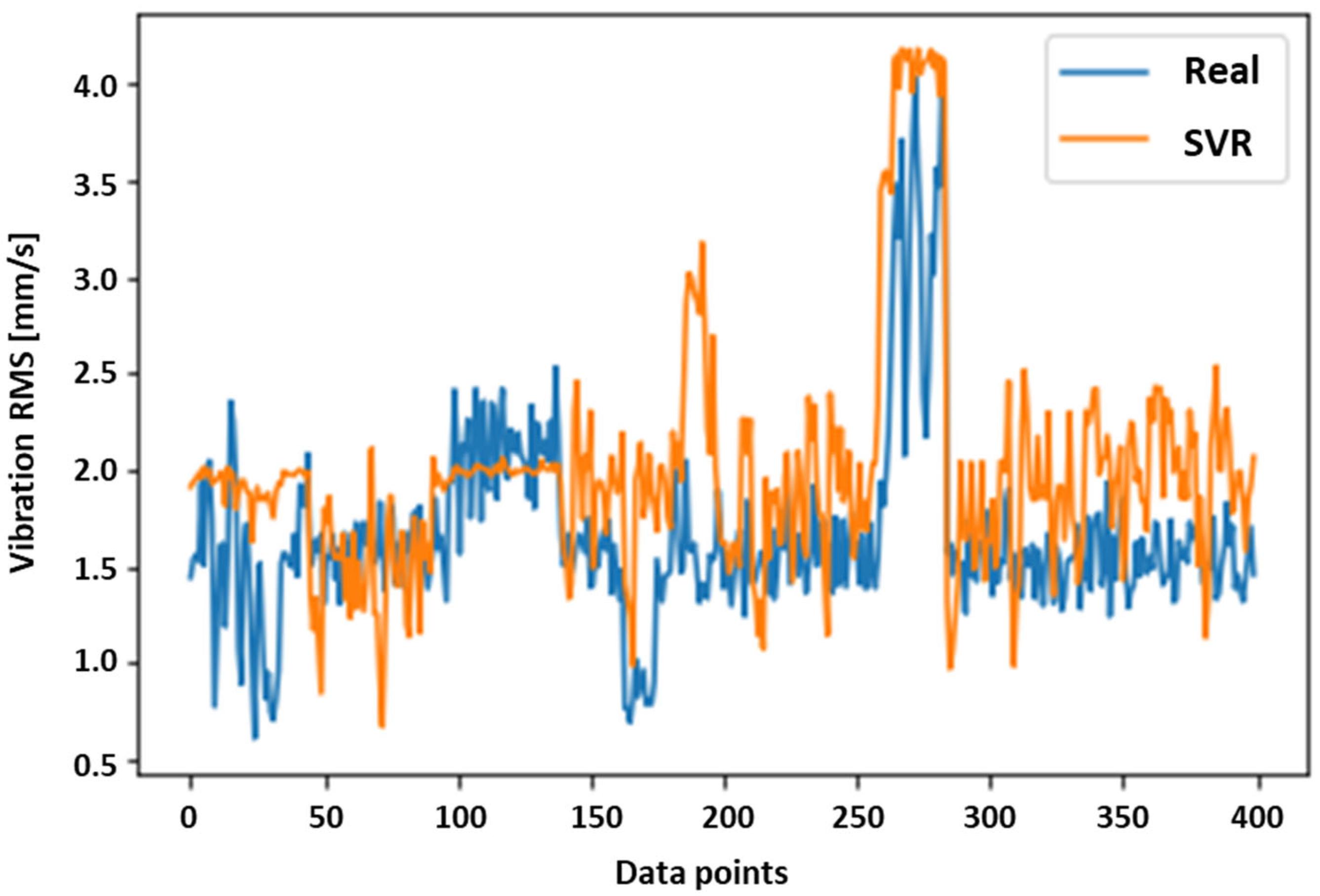
The graphical representation of the SVR RBF’s ability to predict the machine ‘Vibration’ trend is displayed in Figure 10. The SVR trend behaviour in the figure presents four hundred (400) vibration data points formulated based on the input data presented in pseudocode step three. Due to the collection frequency of 5 Hz during the data collection, the visualised 400 data points correspond to approximately 1.3 min of the milling operation.
In conclusion, given by the quantified error scoring results in Table 3 and visualised SVR results in Figure 10, the model’s capability to reflect the given wear indicator of ‘Vibration’ is considered to occur with decent accuracy. Therefore, the ‘Vibration’ parameter should be further tested in addition to more complex prediction algorithms for determining the machine HI index, and ultimately in the remaining life prediction based on the vibration (velocity RMS) parameter.
5. Conclusions
In this paper, a multi-dimensional online data collection system in the context of a peripheral milling machine was established and reported. The data was pre-processed to receive a better understanding of the machine parameters correlating with the milling blade wear phenomenon. The feature reduction methods used gave great confidence in vibration excitation correlation as a wear indicator. As a conclusion from the PCC and PFI results, it is proposed to conjugate additional vibration sensors to the case machine setup and research the wear phenomenon more in-depth in the context. Receiving raw vibration data in multiple dimensions, as well as from different vibration frequency ranges, may result in more profound information for determining the machine health index through vibration signals. Instead of only monitoring a vibration velocity RMS, a higher frequency range monitoring is exploitable to receive an understanding of possible earlier indications or more accurate signs of blade wear. Additionally, other machine-related excitations such as motor torque measures are illustrated to contain information which may be used in predicting machine health index and derived lifetime estimation.
This research also introduced testing of the support vector regression algorithm to analyse vibration parameter behaviour based on the other data collected from the machine’s usage and PLC automation system. The linear, polynomial, and RBF methods were applied to find the most appropriate kernel to adapt the data points in the feature space. The support vector regression method with RBF kernel was used to visualise the prediction of the machine vibration behaviour.
To conclude, the SVR algorithm can predict the vibration signal behaviour rather accurately based on the machine input parameters. As depicted in this research, the vibration signal trend cumulation is unquestionably correlated with the case machine’s usage over time, and with the cutting blade wear behaviour. The supervised machine learning method of SVR can overcome most of the multidimensional data challenges; however, changes in the production recipes create a vast amount of distraction to the process parameter behaviour, which is challenging for the SVR to learn. Milling parameter changes and related vibrational data variation certainly affect the training and test scores of the model; however, the model’s fit, especially with the RBF kernel, appears adequate for vibration amplitude trend prediction over time. Despite the learning challenges, the SVR can achieve acceptable results, and the model’s applicability for prognostic purposes is recognised.
Determining discrete health index monitoring and forecasting an actual remaining useful life (RUL) of the peripheral milling machine were not considered as part of this research due to a lack of data considering the actual wear stages of the milling blades. A hybrid prognostic approach including model-based simulation data implementation, other machine learning techniques, and results of blade wear tests would be seen as beneficial to estimate the HI and derived RUL for the asset. The next research steps will consider these tests with added vibration sensors, diagnostics of other machine excitations to evaluate machine state, as well as the use of other ML prognostic methods to better comply with the recurrent actions occurring in the machines’ operation.
Author Contributions
T.M.: conceptualisation, methodology, validation, formal analysis, investigation, data curation, writing—original draft preparation, writing—review and editing, and visualisation. H.V.: methodology, software, and validation. K.T.K.: supervision, resources, project administration, and funding acquisition. All authors have read and agreed to the published version of the manuscript.
Funding
This research was funded by the Business Finland SNOBI project, grant number 545/31/2020.
Data Availability Statement
Not applicable.
Conflicts of Interest
The authors declare no conflict of interest.
Abbreviations
The following abbreviations are used in this manuscript:
| ANFIS | Adaptive Network-Based Fuzzy Inference System |
| API | Application Programming Interface |
| AUC | Area Under Curve |
| b | Bias |
| BPNN | Back Propagation Neural Network |
| CBM | Condition-Based Maintenance |
| GenSVM | Generalised Multiclass Support Vector Machine |
| HI | Health Index |
| KNN | K-Nearest Neighbour |
| LSSVM | Least Squares Support Vector Machines |
| MAE | Mean Absolute Error |
| ML | Machine Learning |
| MSE | Mean Square Error |
| n | Identification Number of a Single Data Point |
| OEM | Original Equipment Manufacturer |
| PCC | Pearson Correlation Coefficient |
| Phi φ | Dot Product From Input Space to Feature Space |
| PLC | Programmable Logic Controller |
| PPX | Pay-Per-X |
| R2 | Squared Correlation Coefficient |
| RBF | Gaussian Radial Basis Function |
| RF | Random Forest |
| RMS | Root Mean Square |
| ROC | Receiver Operating Characteristics |
| RUL | Remaining Useful Life |
| SVM | Support Vector Machines |
| SVR | Support Vector Regression |
| w | w is A Weight Vector in |
| xi | First Individual Data Point |
| yi | First Individual Data Point of the Comparable Variable |
| Corresponding Arithmetic Mean of the First Sample | |
| Corresponding Arithmetic Mean of the Comparable Variable |
References
- Schroderus, J.; Allan, L.; Menon, K.; Kärkkäinen, H. Towards a Pay-Per-X Maturity Model for Equipment Manufacturing Companies. Procedia Comput. Sci. 2022, 196, 226–234. [Google Scholar] [CrossRef]
- Menon, K. Industrial Internet Enabled Value Creation for Manufacturing Companies; Tampere University: Tampere, Finland, 2020. [Google Scholar]
- Singh, H.; Matharu, G.S.; Dardi, A.K.; Matharu, J.S. Empirical Investigation of Big Data Analytical Tools: Comparative Analysis. In Proceedings of the 2019 3rd International Conference on Trends in Electronics and Informatics (ICOEI), Tirunelveli, India, 23–25 April 2019; pp. 1264–1269. [Google Scholar] [CrossRef]
- Roy, S.K.; Misra, S.; Raghuwanshi, N.S. SensPnP: Seamless Integration of Heterogeneous Sensors with IoT Devices. IEEE Trans. Consum. Electron. 2019, 65, 205–214. [Google Scholar] [CrossRef]
- Li, H.; Wang, W.; Li, Z.; Dong, L.; Li, Q. A novel approach for predicting tool remaining useful life using limited data. Mech. Syst. Signal Process. 2020, 143, 106832. [Google Scholar] [CrossRef]
- Van der Voort, H.; van Bulderen, S.; Cunningham, S.; Janssen, M. Data science as knowledge creation a framework for synergies between data analysts and domain professionals. Technol. Forecast. Soc. Change 2021, 173, 121160. [Google Scholar] [CrossRef]
- Kotsiantis, S.B.; Kanellopoulos, D.; Pintelas, P.E. Data preprocessing for supervised leaning. Int. J. Comput. Sci. 2006, 1, 111–117. [Google Scholar]
- Zhang, Y.; Zhu, K.; Duan, X.; Li, S. Tool wear estimation and life prognostics in milling: Model extension and generalization. Mech. Syst. Signal Process. 2021, 155, 107617. [Google Scholar] [CrossRef]
- Liu, M.; Yao, X.; Zhang, J.; Chen, W.; Jing, X.; Wang, K. Multi-Sensor Data Fusion for Remaining Useful Life Prediction of Machining Tools by IABC-BPNN in Dry Milling Operations. Sensors 2020, 20, 4657. [Google Scholar] [CrossRef] [PubMed]
- Zhang, C.; Yao, X.; Zhang, J.; Jin, H. Tool Condition Monitoring and Remaining Useful Life Prognostic Based on a Wireless Sensor in Dry Milling Operations. Sensors 2016, 16, 795. [Google Scholar] [CrossRef] [Green Version]
- He, Z.; Shi, T.; Xuan, J. Milling tool wear prediction using multi-sensor feature fusion based on stacked sparse autoencoders. Measurement 2022, 190, 110719. [Google Scholar] [CrossRef]
- Usui, E.; Hirota, A.; Masuko, M. Analytical Prediction of Three Dimensional Cutting Process—Part 1: Basic Cutting Model and Energy Approach. J. Eng. Ind. 1978, 100, 222–228. [Google Scholar] [CrossRef]
- Takeyama, H.; Murata, R. Basic Investigation of Tool Wear. J. Eng. Ind. 1963, 85, 33–37. [Google Scholar] [CrossRef]
- Ochoa, L.E.E.; Quinde, I.B.R.; Sumba, J.P.C.; Guevara, A.V.; Morales-Menendez, R. New Approach based on Autoencoders to Monitor the Tool Wear Condition in HSM. IFAC-PapersOnLine 2019, 52, 206–211. [Google Scholar] [CrossRef]
- Panda, S.; Chakraborty, D.; Pal, S. Flank wear prediction in drilling using back propagation neural network and radial basis function network. Appl. Soft Comput. 2008, 8, 858–871. [Google Scholar] [CrossRef]
- Rahimi, M.H.; Huynh, H.N.; Altintas, Y. On-line chatter detection in milling with hybrid machine learning and physics-based model. CIRP J. Manuf. Sci. Technol. 2021, 35, 25–40. [Google Scholar] [CrossRef]
- Chen, Q.; Xie, Q.; Yuan, Q.; Huang, H.; Li, Y. Research on a Real-Time Monitoring Method for the Wear State of a Tool Based on a Convolutional Bidirectional LSTM Model. Symmetry 2019, 11, 1233. [Google Scholar] [CrossRef] [Green Version]
- Wu, D.; Jennings, C.; Terpenny, J.; Gao, R.X.; Kumara, S. A Comparative Study on Machine Learning Algorithms for Smart Manufacturing: Tool Wear Prediction Using Random Forests. J. Manuf. Sci. Eng. 2017, 139, 071018. [Google Scholar] [CrossRef] [Green Version]
- Cheng, Y.; Zhu, H.; Hu, K.; Wu, J.; Shao, X.; Wang, Y. Multisensory Data-Driven Health Degradation Monitoring of Machining Tools by Generalized Multiclass Support Vector Machine. IEEE Access 2019, 7, 47102–47113. [Google Scholar] [CrossRef]
- Benkedjouh, T.; Medjaher, K.; Zerhouni, N.; Rechak, S. Health Assessment and Life Prediction of Cutting Tools Based on Support Vector Regression. J. Intell. Manuf. 2015, 26, 213–223. [Google Scholar] [CrossRef] [Green Version]
- Nee, A.Y.C. Handbook of Manufacturing Engineering and Technology; Springer: Berlin/Heidelberg, Germany, 2015. [Google Scholar] [CrossRef]
- Pecht, M.G.; Kang, M. Prognostics and Health Management of Electronics; IEEE Press: Piscataway, NJ, USA, 2018. [Google Scholar]
- Wan, Z.; Xu, Y.; Šavija, B. On the Use of Machine Learning Models for Prediction of Compressive Strength of Concrete: Influence of Dimensionality Reduction on the Model Performance. Materials 2021, 14, 713. [Google Scholar] [CrossRef]
- Gruosso, G.; Gajani, G.S.; Ruiz, F.; Valladolid, J.D.; Patino, D. A Virtual Sensor for Electric Vehicles’ State of Charge Estimation. Electronics 2020, 9, 278. [Google Scholar] [CrossRef] [Green Version]
- Chang, C.; Lin, C. LIBSVM: A Library for Support Vector Machines. ACM Trans. Intell. Syst. Technol. 2013, 2, 27. [Google Scholar] [CrossRef]
- Santos, C.E.D.S.; Sampaio, R.C.; Coelho, L.D.S.; Bestard, G.A.; Llanos, C.H. Multi-objective adaptive differential evolution for SVM/SVR hyperparameters selection. Pattern Recognit. 2020, 110, 107649. [Google Scholar] [CrossRef]
- Rivas-Perea, P.; Cota-Ruiz, J.; Chaparro, D.G.; Venzor, J.A.P.; Carreón, A.Q.; Rosiles, J.G. Support Vector Machines for Regression: A Succinct Review of Large-Scale and Linear Programming Formulations. Int. J. Intell. Sci. 2013, 03, 5–14. [Google Scholar] [CrossRef] [Green Version]
- Sabzekar, M.; Hasheminejad, S.M.H. Robust regression using support vector regressions. Chaos Solitons Fractals 2021, 144, 110738. [Google Scholar] [CrossRef]
- Stapelberg, R.F. Handbook of Reliability, Availability, Maintainability and Safety in Engineering Design; Springer: Berlin/Heidelberg, Germany, 2009. [Google Scholar] [CrossRef]
- Boyes, H.; Hallaq, B.; Cunningham, J.; Watson, T. The industrial internet of things (IIoT): An analysis framework. Comput. Ind. 2018, 101, 1–12. [Google Scholar] [CrossRef]
- Omri, N.; Al Masry, Z.; Mairot, N.; Giampiccolo, S.; Zerhouni, N. Industrial data management strategy towards an SME-oriented PHM. J. Manuf. Syst. 2020, 56, 23–36. [Google Scholar] [CrossRef]
- Müller, A.C.; Guido, S. Introduction to Machine Learning with Python and Scikit-Learn. 2015. Available online: http://kukuruku.co/hub/python/introduction-to-machine-learning-with-python-andscikit-learn (accessed on 1 June 2022).
- Kadiyala, A.; Kumar, A. Applications of Python to evaluate environmental data science problems. Environ. Prog. Sustain. Energy 2017, 36, 1580–1586. [Google Scholar] [CrossRef]
- Géron, A. Hands-On Machine Learning with Scikit-Learn & TensorFlow; O’Reilly Media, Inc.: Sebastopol, CA, USA, 2019; Volume 53. [Google Scholar]
- Tschätsch, H. Applied Machining Technology; Springer: Berlin/Heidelberg, Germany, 2009; pp. 5–23. [Google Scholar] [CrossRef]
- Adler, J.; Parmryd, I. Quantifying colocalization by correlation: The Pearson correlation coefficient is superior to the Mander’s overlap coefficient. Cytom. Part A 2010, 77A, 733–742. [Google Scholar] [CrossRef]
- Jiang, J.-R.; Kao, J.-B.; Li, Y.-L. Semi-Supervised Time Series Anomaly Detection Based on Statistics and Deep Learning. Appl. Sci. 2021, 11, 6698. [Google Scholar] [CrossRef]
- Molnar, C.; Freiesleben, T.; König, G.; Casalicchio, G.; Wright, M.N.; Bischl, B. Relating the Partial Dependence Plot and Permutation Feature Importance to the Data Generating Process. arXiv 2021, arXiv:2109.01433. [Google Scholar] [CrossRef]
- Van Calster, B.; Wynants, L.; Collins, G.S.; Verbakel, J.Y.; Steyerberg, E.W. ROC curves for clinical prediction models part 3. The ROC plot: A picture that needs a 1000 words. J. Clin. Epidemiol. 2020, 126, 220–223. [Google Scholar] [CrossRef]
- Hand, D.J. Measuring classifier performance: A coherent alternative to the area under the ROC curve. Mach. Learn. 2009, 77, 103–123. [Google Scholar] [CrossRef] [Green Version]
- Carter, J.V.; Pan, J.; Rai, S.N.; Galandiuk, S. ROC-ing along: Evaluation and interpretation of receiver operating characteristic curves. Surgery 2016, 159, 1638–1645. [Google Scholar] [CrossRef]
- Blanco, V.; Puerto, J.; Rodriguez-Chia, A.M. On p-Support Vector Machines and Multidimensional Kernels. J. Mach. Learn. Res. 2020, 21, 469–497. [Google Scholar]
- Chicco, D.; Warrens, M.J.; Jurman, G. The coefficient of determination R-squared is more informative than SMAPE, MAE, MAPE, MSE and RMSE in regression analysis evaluation. PeerJ Comput. Sci. 2021, 7, e623. [Google Scholar] [CrossRef] [PubMed]
- Klein, S.; Schorr, S.; Bähre, D. Quality Prediction of Honed Bores with Machine Learning Based on Machining and Quality Data to Improve the Honing Process Control. Procedia CIRP 2020, 93, 1322–1327. [Google Scholar] [CrossRef]
- Teti, R.; Segreto, T.; Caggiano, A.; Nele, L. Smart Multi-Sensor Monitoring in Drilling of CFRP/CFRP Composite Material Stacks for Aerospace Assembly Applications. Appl. Sci. 2020, 10, 758. [Google Scholar] [CrossRef] [Green Version]
- Wan, X. Influence of feature scaling on convergence of gradient iterative algorithm. J. Phys. Conf. Ser. 2019, 1213, 032021. [Google Scholar] [CrossRef] [Green Version]
Figure 1.
The peripheral milling process’s main physical components are (a) AC electric motor, (b) gearbox, (c) shaft, (d) spindle, and (e) milling position (x-axis direction feed). The data flow to the internet-connected data collection system is connected through the integrated PLC system and Azure Cosmos MongoDB API.

Figure 2.
Data creation and acquisition flow.

Figure 3.
Pearson correlation heatmap illustrating the numeric and visual correlation between the scaled-down parameters.
Figure 3.
Pearson correlation heatmap illustrating the numeric and visual correlation between the scaled-down parameters.

Figure 4.
Given conditions to the PFI algorithm.

Figure 5.
Permutation feature importance results.

Figure 6.
Feature reduction pipeline with PCC and PFI methods resulting in added wear behaviour knowledge.
Figure 6.
Feature reduction pipeline with PCC and PFI methods resulting in added wear behaviour knowledge.

Figure 7.
Two-dimensional representation of hyperplane behaviour with epsilon and C-values ε = 0.1, C = 100.
Figure 7.
Two-dimensional representation of hyperplane behaviour with epsilon and C-values ε = 0.1, C = 100.

Figure 8.
Three-dimensional scatter plot with SVR RBF hyperplane from two different viewpoints (a,b).
Figure 8.
Three-dimensional scatter plot with SVR RBF hyperplane from two different viewpoints (a,b).

Figure 9.
The pseudocode of the SVR algorithm.

Figure 10.
Support Vector Regression (RBF; ε = 0.1, C = 100) comparison with real vibration signal.


Table 1.
Collected data from manual setup data and PLC automation control.
| Manual Setup Data | PLC Automation Control |
|---|---|
| Milling Part ID | Cutting Speed Set Point [220–240 rpm] |
| Profile Height [70–200 mm] | Feed Rate Set Point [5000–8000 mm/min] |
| Profile Length [6000–23,800 mm] | Feed Motor Torque Set Point [% of nominal] |
| Profile Thickness [5–30 mm] | Frame Position Set Point [0…3] |
| Profile Type [I or L] | Machine Active [T/F] |
| Spindle Position [0…3] | Mill Depth Set Point [1.5–3.03 mm] |
| Tool Number [1 or 2] | Milling Status [T/F] |
| Time Stamp [yyyy-mm-dd-hh-mm-ss] |
Table 2.
Calculated and measured data from the manufacturing process.
| Calculated Parameters | Measured Parameters |
|---|---|
| Cutting Speed Ratio [0…1] | Cutting Speed [rpm] |
| Feed Rate Ratio [0…1] | Feed Rate [mm/min] |
| Num. Of Tool Rows Used [1 or 2] | Milling End Time [yyyy-mm-dd-hh-mm-ss] |
| ToolRows0.MilledMeters [m] | Milling Start Time [yyyy-mm-dd-hh-mm-ss] |
| ToolRows0.MilledTime [s] | Spindle Motor Torque [% of nominal] |
| ToolRows0.Used [T/F] | Vibration [mm/s RMS] |
| ToolRows1.MilledMeters [m] | |
| ToolRows1.MilledTime [s] | |
| ToolRows1.Used [T/F] | |
| ToolRows2.MilledMeters [m] | |
| ToolRows2.MilledTime [s] | |
| ToolRows2.Used [T/F] | |
| ToolRows3.MilledMeters [m] | |
| ToolRows3.MilledTime [s] | |
| ToolRows3.Used [T/F] | |
| ToolRowsUsed.MaxMilledMeters [m] | |
| ToolRowsUsed.AvgMilledMeters [m] | |
| ToolRowsUsed.MinMilledMeters [m] |
Table 3.
Model error scoring comparison with ε = 0.1, C = 100.
| Error Scoring Metric | Linear | SVR POLY | SVR RBF |
|---|---|---|---|
| Train score R2 | 0.649464505 | 0.819797848 | 0.856560515 |
| Test score R2 | 0.646896683 | 0.803223516 | 0.846645929 |
| Train mean absolute error (MAE) | 0.080181311 | 0.056275051 | 0.049610738 |
| Train MSE [%] | 0.010790393 | 0.006013242 | 0.004686307 |
Disclaimer/Publisher’s Note: The statements, opinions and data contained in all publications are solely those of the individual author(s) and contributor(s) and not of MDPI and/or the editor(s). MDPI and/or the editor(s) disclaim responsibility for any injury to people or property resulting from any ideas, methods, instructions or products referred to in the content. |
© 2023 by the authors. Licensee MDPI, Basel, Switzerland. This article is an open access article distributed under the terms and conditions of the Creative Commons Attribution (CC BY) license (https://creativecommons.org/licenses/by/4.0/).
Share and Cite
MDPI and ACS Style
Mäkiaho, T.; Vainio, H.; Koskinen, K.T. Wear Parameter Diagnostics of Industrial Milling Machine with Support Vector Regression. Machines 2023, 11, 395. https://doi.org/10.3390/machines11030395
AMA Style
Mäkiaho T, Vainio H, Koskinen KT. Wear Parameter Diagnostics of Industrial Milling Machine with Support Vector Regression. Machines. 2023; 11(3):395. https://doi.org/10.3390/machines11030395
Chicago/Turabian StyleMäkiaho, Teemu, Henri Vainio, and Kari T. Koskinen. 2023. "Wear Parameter Diagnostics of Industrial Milling Machine with Support Vector Regression" Machines 11, no. 3: 395. https://doi.org/10.3390/machines11030395
Note that from the first issue of 2016, this journal uses article numbers instead of page numbers. See further details here.