Co-Simulation Modeling and Multi-Objective Optimization of Dynamic Characteristics of Flow Balancing Valve

Abstract

The poor dynamic characteristics of the flow balance valve used in a ship’s HVAC system are the main reasons for the hydraulic imbalance and high energy consumption of the system. A new adjustable dynamic flow balance valve structure is designed, which is composed of a self-operated pressure regulator and an electric V-shaped ball valve in series. When the V-shaped ball valve is fully opened at the 20 t/h flow level, the dynamic characteristics of the flow balance valve cannot meet the requirements. A new co-simulation method that combines MATLAB/Simulink and the UDF dynamic grid is proposed to study the dynamic characteristics of a flow balance valve with a 20 t/h flow rate under different pressure drop step signal interference. When the calculation of each micro-element time converges, the valve core motion parameters, the pressure boundary conditions, the valve core axial medium force, and the valve outlet flow are interactively transmitted in the two simulation environments. The discrepancy between the co-simulation and test results is less than 5%, which verifies the accuracy of the co-simulation model. Aiming at the most severe dynamic characteristic working condition where the pressure drop is stepped from 30 to 300 kPa, the influence of different structural parameters on the dynamic characteristics of the balance valve is analyzed. A new surrogate model combining RSM and RBF with the co-simulation method improves the optimization efficiency and fitting accuracy. To improve the convergence of the traditional NSGA-II algorithm, key structural parameters are optimized by combining the NSGA-II algorithm and SDR. The test results show that the dynamic characteristics of the optimized valve are improved, the discrepancy between the stabilized flow rate and 20 t/h does not exceed 4.5%, and the flow is relatively constant. Therefore, the proposed co-simulation and optimization method can be applied to the dynamic characteristic prediction of self-operated valves, such as dynamic flow balance valves, to provide guidance for developing high-precision self-operated valves.

1. Introduction

The HVAC (heating ventilating and air conditioning) system of modern ships is changing to an integrated and regionalized supply mode. In the actual regionalized and integrated supply of heating or cooling, the pipeline network is prone to the phenomenon of hydraulic imbalance due to factors such as the design, changes in the number of users, and differences in the location of end users. At present, the most common method to solve the problem of hydraulic imbalance in the HVAC system is to install a dynamic flow balance valve in the front section of each user. However, the existing dynamic flow balance valve products generally have problems such as poor dynamic characteristics and narrow control range [1,2,3,4,5]. The balance valve usually needs to be equipped with a larger pump source for auxiliary control, which will cause the power system to take up too much space. In addition, the frequency conversion pump requires the frequency converter to adjust the pump speed repeatedly, which easily cause the problems of high noise and high energy consumption. Therefore, the development of dynamic flow balance valve products with good dynamic characteristics can improve the operating efficiency of the HVAC system in the cabin, reduce the volume of the power system, and provide a comfortable working environment for the cabin crew. At the same time, the exploration of high-precision numerical simulation methods and efficient optimization methods for the dynamic characteristics of balance valves can guide the research and development of such self-operated valves.

When the pressure drop of the dynamic flow balance valve changes, due to the rise or fall of the pressure before the valve, the self-operated pressure regulator in the balance valve will automatically change the opening. Due to the unbalanced force on the pressure-sensitive piston, when the pressure regulator is adjusted completely, the flow in the balancing valve will remain relatively equal to the flow before the differential pressure change. The better the dynamic characteristics of the dynamic flow balancing valve from unbalanced to balanced overall dynamic engineering, the better the control performance of the district heating system. Therefore, it is very necessary to study the dynamic characteristics of the dynamic flow balance valve under the condition of the differential pressure step change signal. It is the focus of this work to explore the high-precision joint numerical simulation method and effective optimization method for the dynamic characteristics of the dynamic flow balance valve. Dynamic flow balancing valves are self-operated valves, and most of the existing numerical simulation methods for studying self-operated valves use a single numerical simulation software, resulting in a large discrepancy between the simulation results and the test. Moreover, the dynamic performance of the existing dynamic flow balance valve products is poor, and there is a lack of research on its optimization.

The dynamic flow balance valve is a kind of self-operated valve. There are many studies on the dynamic characteristics of self-operated valves. The main research methods are based on one-dimensional numerical simulation software alone, such as Simulink and AMEsim, or using CFD software alone to analyze the dynamic characteristics of self-operated valves. Li et al. [6] used dynamic mesh technology to simulate the motion of the spool and performed transient CFD simulations to analyze its dynamic characteristics. The overall discrepancy between the simulation and experimental data does not exceed 15%, which has the problem of a large amount of calculation and low overall simulation accuracy. According to the dynamic characteristics of the valve actuator under a certain volume constraint, Liu et al. [7] used MATLAB/Simulink software to obtain the dynamic characteristic curve of the valve closing speed when the actuator failed. The experimental results show that the failure closing time of the valve is consistent with the theoretical calculation value, and the end vibration is within the allowable range. Lei et al. [8] studied the flow model and dynamic characteristics of the poppet relief valve. The dynamic model including the aforementioned flow model of the poppet valve is established with consideration of the fluid forces caused by the valve body motion and flow rate variation. The dynamic characteristics of the different working conditions of the poppet relief valve are obtained using this method. Arslan et al. [9] used dynamic mesh technology to carry out a dynamic numerical simulation of the flow process in the pressure-regulating globe valve and obtained the valve closing time. The conclusion that the closing time is related to the coefficient of friction was obtained. Liu et al. [10] introduced the function of the load control valve, simulated the dynamic characteristics of the load control valve, obtained the load pressure compensation characteristics, and optimized the compensation hole size. Based on the transient CFD method and moving mesh technique, Ye et al. [11] established a transient hydrogen flow model of the check valve and studied the effect of different spool head angles on the closing impact. The optimal design value of the spool head angle was obtained. Zang et al. [12] proposed a method to study the dynamic characteristics of the main steam valve with different inlet port diameters using the dynamic mesh technology and analyzed the pressure of the pilot valve during the opening process. However, this method has the problems of large calculation time cost and large local numerical error. Song et al. [13] studied the working mechanism of the safety valve using the method of refined modeling and dynamic mesh and optimized its performance using the surrogate model. Tang et al. [14] used digital twin technology to study the dynamic characteristics of a precision spool valve in an electro-hydraulic servo control system. Experiments have proved that this method has high accuracy in most working conditions, but it has the problem of high cost of digital twins and difficulty in accurate full-scale modeling. The above works of literature generally use a single one-dimensional numerical simulation or dynamic grid method alone to calculate the dynamic characteristics of the valve; generally, the simulation accuracy is not high (the error exceeds 5%), the three-dimensional dynamic grid method has a high calculation time cost, and it is difficult to converge problems.

Some high-performance district heating systems put forward higher requirements on the dynamic characteristics of the dynamic flow balance valve, so it is necessary to study the optimization method of the dynamic characteristics of the balance valve. The dynamic performance of the balance valve is usually determined by the overshoot, transition time, and residual difference, so this involves a multi-objective optimization problem. The existing literature lacks the multi-objective optimization of dynamic flow balance valves, but there are many kinds of literature on the multi-objective optimization of mechanical properties, which can provide a reference. Wang et al. [15] proposed a surrogate model combined with the finite element method (FEM) and computational fluid dynamics (CFD) analysis to improve optimization efficiency. The optimized connecting rod butterfly valve structure is obtained using this method. Mao et al. [16] introduce a vector of relaxation factors to soften hard constrained boundaries, which had no feasible solution before. To maintain driving stability under complex conditions, a multi-objective optimization method with the online updating of weight coefficients is proposed. The optimal control method for the vehicle was obtained. Fan et al. [17] proposed an improved constraint handling mechanism and combined it with a decomposition-based multi-objective evolutionary algorithm to solve constrained multi-objective optimization problems; the efficiency of this improved optimization method is verified using the test function. Jiang et al. [18], based on the Kriging surrogate model and the NSGA-II algorithm, carried out a multi-objective lightweight optimization of the dump truck compartment and used the entropy weight TOPSIS method to select the optimal design of the dump truck from the Pareto solution.

By consulting the literature on the simulation and experimental research of the performance of the self-operated valve, it is found that there are few experimental and numerical studies of the dynamic characteristics of the flow balance valve, and the discrepancy between simulation and test is generally 8~10%, which will be difficult to guide the design of high-precision dynamic flow balancing valves. In addition, there is no literature on the multi-objective optimization of the structural parameters of the dynamic flow balance valve. Therefore, to solve the disadvantages of a single simulation environment, a new co-simulation method that combines MATLAB/Simulink and the UDF dynamic grid was built to improve simulation accuracy and computational efficiency. When the calculation of each micro-element time converges, the valve core motion parameters, the pressure boundary conditions, the valve core axial medium force, and the valve outlet flow are interactively transmitted in the two simulation environments. The simulation results are compared with experimental results to verify the accuracy of the co-simulation model. Aiming at the problem that when the V-shaped ball valve is fully opened at the 20 t/h flow level, the dynamic characteristics of the adjustable dynamic flow balance valve cannot meet the requirements, the influence of structural parameters on the dynamic characteristics of the balance valve is analyzed. A new weighted ratio combined surrogate model that comprehensively considers RSM (response surface methodology) and RBF (radial basis function) is combined with the co-simulation method to improve optimization efficiency and fitting accuracy. To improve the convergence of the traditional NSGA-II algorithm, the volume of the left and right volume chambers of the diaphragm, the spring stiffness coefficient, the diameter of the pressure guide hole, and the outer diameter of the diaphragm are optimized by combining the NSGA-II algorithm and SDR (strengthening dominance relation). The dynamic characteristics test of the optimized balance valve was performed to verify the feasibility of the optimization method.

2. Establishment of Dynamic Model of Dynamic Flow Balance Valve

2.1. Structural Characteristics and Working Principle of the Valve

The dynamic flow balance valve is composed of a pressure regulator and V-shaped ball valve in series. The three-dimensional model is shown in Figure 1, and the structure principle and main parts are shown in Figure 2.

Keeping the V-shaped ball valve at a certain opening, the pressure regulator can keep the pressure drop between the front and rear of the ball valve constant, thereby making the flow rate of the ball valve constant. Within this range, the outlet flow of the valve remains relatively constant.

2.2. Establishment of Dynamic Model of Dynamic Flow Balance Valve

The differential equation of motion of the pressure regulator valve core diaphragm motion component in the axial direction can be expressed as [7]:

$$m\ddot{x}=F_{\mathrm{p}}-F_{\mathrm{k}}-F_{\mathrm{O}}-F_{\mathrm{d}}-F_{\mathrm{Z}}-F_{\mathrm{m}}$$

(1)

where F_p is the axial hydraulic differential force of the diaphragm; F_k is the spring force; F_O is the friction force of the O-ring; F_d is the unbalanced force on both ends of the valve core; F_Z is the viscous damping force; and F_m is the rebound force of the diaphragm.

$$\begin{array}{cc}{F}_p& =(P_2{}^{\prime }-P_3{}^{\prime })A\hfill \\ & =(P_2{}^{\prime }-P_3{}^{\prime })\left[\frac{\pi (D_m{}^2+D_m{d}_m+d_m{}^2)}{12}-\frac{\pi D^2}{4}\right]\hfill \end{array}$$

(2)

where A is the effective area of the diaphragm; P₂’ is the pressure in the left chamber of the diaphragm; and P₃’ is the pressure in the right chamber of the diaphragm. D_m is the diameter of the diaphragm closure; d_m is the diameter of the diaphragm dome; and D is the outer diameter of the valve core.

$$\begin{array}{ll}{F}_d& =(P_1-P_2)A_{\mathrm{s}}\\ & =(P_1-P_2)\pi (D^2-D_1{}^2)/4\end{array}$$

(3)

where A_s is the end face area; and D₁ is the inner diameter of the valve core. The formula for calculating the friction force generated by the pre-compression of the O-ring is [19]:

$$F_1=\frac{0.2{\pi }^{2}feE{D}_{e}d}{1-{\mu }^2}$$

(4)

where f is the coefficient of friction; d is the diameter of the O-ring section; D_e is the outer diameter of the O-ring; e is the compression ratio; μ is the Poisson’s ratio; and E is the elastic modulus. The hydraulic pressure drop on both sides of the O-ring is P₁–P₃′, and the friction force expression caused by the pressure drop on both sides is [19]:

$$F_2(P_1,P_3{}^{\prime })=\frac{f\pi (1+\mu )}{1-{\mu }^2}(P_1-P_3{}^{\prime })D_{e}d$$

(5)

The expression of the total sliding friction force of the O-ring is [19]:

$$\begin{array}{ll}{F}_{\mathrm{h}}(P_1,P_3{}^{\prime })& =F_1+F_2(P_1,P_3{}^{\prime })\\ & =\frac{f\pi D_{\mathrm{e}}d}{1-{\mu }^2}[0.2\pi eE+\mu (1+\mu )(P_1-P_3{}^{\prime })]\end{array}$$

(6)

In reference [19,20], the calculation model of the total friction force of the O-ring considering the static friction and sliding friction is:

$$F_{\mathrm{O}}(P_1,P_3{}^{\prime },\dot{x})=\{\begin{array}{ll}{F}_{\mathrm{h}}(P_1,P_3{}^{\prime })\left[1.5+\mathrm{sgn}(\dot{x})\right],& \dot{x}=0\\ F_{\mathrm{h}}(P_1,P_3{}^{\prime })\mathrm{sgn}(\dot{x}),& \dot{x}\ne 0\end{array}$$

(7)

where v is the valve core assembly speed.

$$F_{\mathrm{k}}=(x_0+x)k$$

(8)

where k is the spring stiffness coefficient; x₀ is the spring pre-compression; and x is the spool displacement.

$$F_{\mathrm{Z}}=B\dot{x}$$

(9)

$$B=\pi \mu D_{0}L/\delta$$

(10)

where B is the viscous resistance coefficient.

The diaphragm rebound force is regarded as a function of the displacement of the valve core, which is expressed as F_m(x). The F_m(x) curve is shown in Figure 3.

Equation (1) can be written as:

$$\begin{array}{l}m\ddot{x}=(P_2{}^{\prime }-P_3{}^{\prime })A-k(x_0+x)-F_{\mathrm{O}}(P_1,P_3{}^{\prime },\dot{x})\\ -(P_1-P_2)A_{\mathrm{s}}-B\dot{x}-F_{\mathrm{m}}(x)\end{array}$$

(11)

The flow characteristic of the valve port of the pressure regulator is a flat plate quick-opening type. The flow equation of the pressure regulator can be obtained as [8]:

$$Q_1=C_{\mathrm{d}}{}_1\pi D(h-x)\sqrt{2(P_1-P_2)/\rho }$$

(12)

where C_d1 is the flow coefficient of the pressure regulator, and h is the full stroke of the valve core. The flow equation of the V-type ball valve is [8]:

$$Q_2=C_{\mathrm{d}}{}_2{A}_2\sqrt{2(P_2-P_3)/\rho }$$

(13)

where C_d2 is the flow coefficient of the V-shaped ball valve; A₂ is the flow area of the ball valve; and P₃ is the pressure after the valve.

3. Co-Simulation Analysis of Dynamic Characteristics and Control Accuracy

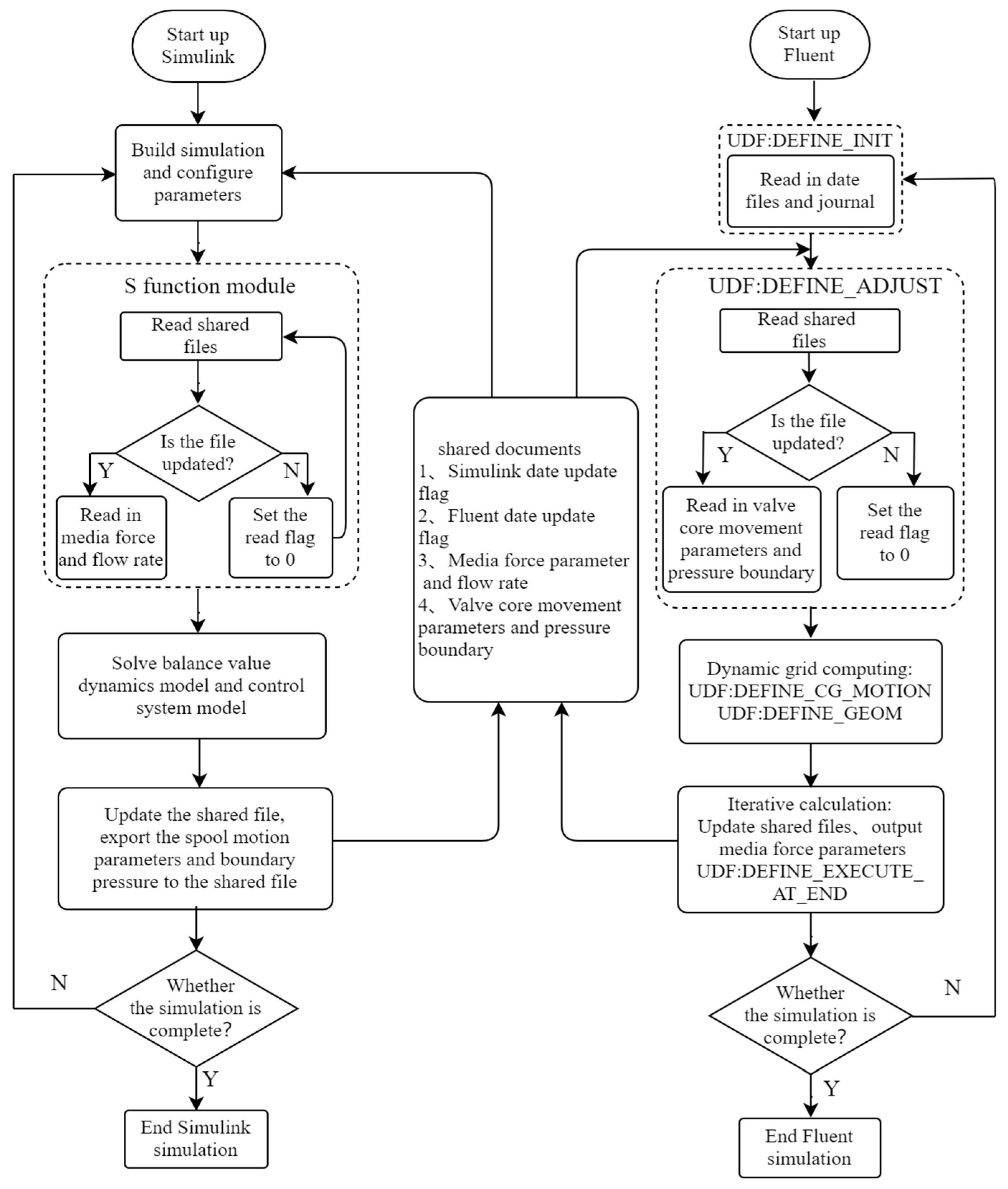
3.1. Establishment of Co-Simulation Model

All operations dealing with the interface of FLUENT/UDF are compiled into an independent S-function program, which can be directly embedded into the dynamic system simulation model in Simulink as an embedded MATLAB function module. This function takes the motion parameters of the valve core assembly and the inlet and outlet pressure boundary parameters as the input and takes the axial medium force of the valve core assembly and the valve flow as the output. The concrete realization method of its co-simulation is shown in Figure 4.

The parameters passed by the S program to FLUENT/UDF are divided into two categories; one is the boundary condition parameters set by GUI, which is passed by modifying the Journal file, and the other is the parameters used to calculate the motion law of the moving grid in UDF. As the interface form of UDF is fixed, it is only used to pass parameters with the FLUENT/UDF computing environment, and no additional parameter transmission is provided. Therefore, these parameters need to be passed through shared memory or shared parameter files, and the memory needs to be agreed upon as well as the address or file name and defined format of the shared data.

Based on the above ideas, the MATLAB/Simulink–FLUENT/UDF co-simulation model was developed, as shown in Figure 5. The resultant force of the unbalanced force at both ends of the valve core and the hydraulic differential force on both sides of the diaphragm is calculated and derived using FLUENT/UDF and read using the S function, expressed as F_q; the valve flow Q_out is calculated and derived using FLUENT/UDF and read using the S-function. Equation (11) can be written as:

$$m\ddot{x}=F_{\mathrm{q}}-k(x_0+x)-F_{\mathrm{O}}(P_1,P_3{}^{\prime },\dot{x})-B\dot{x}-F_{\mathrm{m}}(x)$$

(14)

3.2. Selection of CFD Turbulence Model and Meshing of Flow Channels

To study the flow characteristics and flow control accuracy of the dynamic constant flow valve in its working area, simulation experiments were carried out. CFD (computational fluid dynamics) is used to study the internal flow characteristics. The fluid flow in the valve follows the conservation of momentum and conservation of mass.

The large eddy simulation (LES) turbulence model based on the governing equations of fluid flow, which combines direct numerical simulation and Reynolds time-average method, can effectively capture the small and medium scale of the flow field. The comparison between the test and simulation verifies that the LES has high accuracy in calculating the flow rate [21,22,23,24]. It can obtain more complete transient flow field characteristics, and the computer requirements are much lower than the direct numerical simulation method. Therefore, in this paper, the LES is used as the turbulence model, the no-slip wall boundary condition is used to calculate the flow near the wall, and the SIMPLE solution method is used. The unsteady N-S equation is filtered to obtain the governing equation of the large eddy simulation. The filtering process effectively filters out the small eddies whose scales are smaller than the filter width (or grid scale).

Filtering N-S equation using discrete volume equation [25]:

$$\frac{\partial \overline{u_i}}{\partial t}+\frac{\partial \overline{u_i}\overline{u_j}}{\partial \overline{x_j}}=-\frac{1}{\rho }\frac{\partial \overline{p}}{\partial x_i}+\nu \frac{{\partial }^2\overline{x_i}}{\partial x_j\partial x_j}+\frac{\partial \overline{{\tau }_{ij}}}{\partial x_j}$$

(15)

Sublattice stress:

$$\overline{{\tau }_{ij}}=(\overline{u_i}\overline{u_j}-\overline{u_i{u}_j})$$

(16)

To close the system of equations, according to Smagorinsky’s basic SGS model, it is assumed that the SGS Reynolds stress has the following form:

$${\tau }_{ij}=-2{\nu }_t\overline{s_{ij}}+\frac{1}{3}{\tau }_{kk}{\delta }_{ij}$$

(17)

where δ_ij is the unit tensor, μ_i is the sublattice turbulent viscosity coefficient, and $\overline{s_{ij}}$ is the component of the strain tensor at scale.

$$\overline{s_{ij}}=\frac{1}{2}(\frac{\partial \overline{u_i}}{\partial x_j}+\frac{\partial \overline{u_j}}{\partial x_i})$$

(18)

As the full stroke of the valve core h is 12 mm, the maximum travel of the unilateral valve core is 6 mm, which is less than ±5% of the outer diameter of its closure. According to the relevant literature, its effective area can be regarded as unchanged within this travel range. The diaphragm is simplified to a piston with the same effective area for the simulation of the FLUENT/UDF fluid dynamics environment.

According to the respective advantages of tetrahedral and hexahedral meshes, the flow channel model mesh of the dynamic flow balance valve is divided by a tetrahedral/hexahedral hybrid mesh, which is shown in Figure 6. At the same time, a reasonable grid height of the first layer of the boundary layer is selected so that the grid nodes fall in the logarithmic law region to avoid the discrepancy of the numerical calculation results caused by the grid nodes falling on the viscous bottom layer. Considering the influence of the boundary layer, five boundary layers are divided on the surface of valve body and pipeline. Take the grid height of the first layer as 0.54 mm and the increase rate as 1.2.

The boundary conditions are shown in Equation (19):

$$\{\begin{array}{l}{P}_1=50 \mathrm{kPa}~320 \mathrm{kPa}\\ P_2=20 \mathrm{kPa}\end{array}$$

(19)

The grid independence is shown in

Table 1. Independence test of flow channel grid.

Grid Type	Nodes	Grid Cells	Q (t/h)
grid 1	375,843	1,724,088	18.213
grid 2	533,730	2,535,383	18.931
grid 3	973,361	2,993,506	19.301
grid 4	1,353,821	3,386,235	19.321

. Through the grid independence test, it is finally determined that the number of nodes in the fully open grid of the flow channel in the dispensing device is 973,361, and the number of cells is 2,993,506.

3.3. Co-Simulation Results of Dynamic Characteristics and Control Accuracy

Give the co-simulation model the interference of the step-change signal of pressure drop from 30 kPa to different pressure drops. In the simulation environment of MATLAB/Simulink, the velocity and displacement curves of the valve core assembly are obtained, as shown in Figure 7, Figure 8 and Figure 9.

The boundary conditions of the pressure difference from 30 to 60, 90, 150, 210, and 300 kPa are applied to the co-simulation model, and the dynamic characteristic curves of the different working conditions are obtained, as shown in Figure 10. According to the numerical simulation results, it can be obtained that the flow dynamic characteristic curve of the valve with a pressure drop from 30 to 300 kPa has the longest transition time and the largest residual and overshoot. After the valve is stabilized, the discrepancy from 20 t/h exceeds 10%, and the effect of constant flow cannot be achieved. The pressure drop from 30 to 300 kPa is, therefore, the most severe boundary condition.

Derive the calculation results of the UDF dynamic mesh transient flow field at different times in FLUENT with the boundary condition pressure drop from 30 to 300 kPa, as shown in Figure 11, Figure 12 and Figure 13.

4. Test Results and Precision Analysis

4.1. Comparison between Experiment and Simulation

The dynamic characteristic performance of the dynamic flow balance valve is tested. The test system, acquisition system, pressure, and flow instruments are shown in Figure 14.

The dynamic characteristic curves of the co-simulation and test under the disturbance of the pressure drop from 30 to 300 kPa are compared, as shown in Figure 15. The maximum flow value of the dynamic characteristic curve obtained by the test is 26.63 t/h, and the transition time is 0.63 s, and the stable flow value is 22.15 t/h. The maximum flow value of the dynamic characteristic curve obtained by the co-simulation is 25.83 t/h, the transition time is 0.57 s, and the stable flow value is 21.72 t/h. The discrepancy between the three dynamic characteristic curve indexes of the co-simulation and the experiment is small.

4.2. Analysis of Valve Performance Based on Test Data

According to Figure 16, it can be seen that the overshoot δ of the dynamic characteristic curve exceeds 4 t/h, the transition time ts exceeds 0.55 s, the stable flow rate is 22.1 t/h, and the relative discrepancy from 20 t/h reaches 10.5%, which cannot meet the requirement of nearly constant flow. Therefore, the originally designed valve has poor performance and needs to be optimized.

5. Optimization of Performance of Dynamic Flow Balance Valve

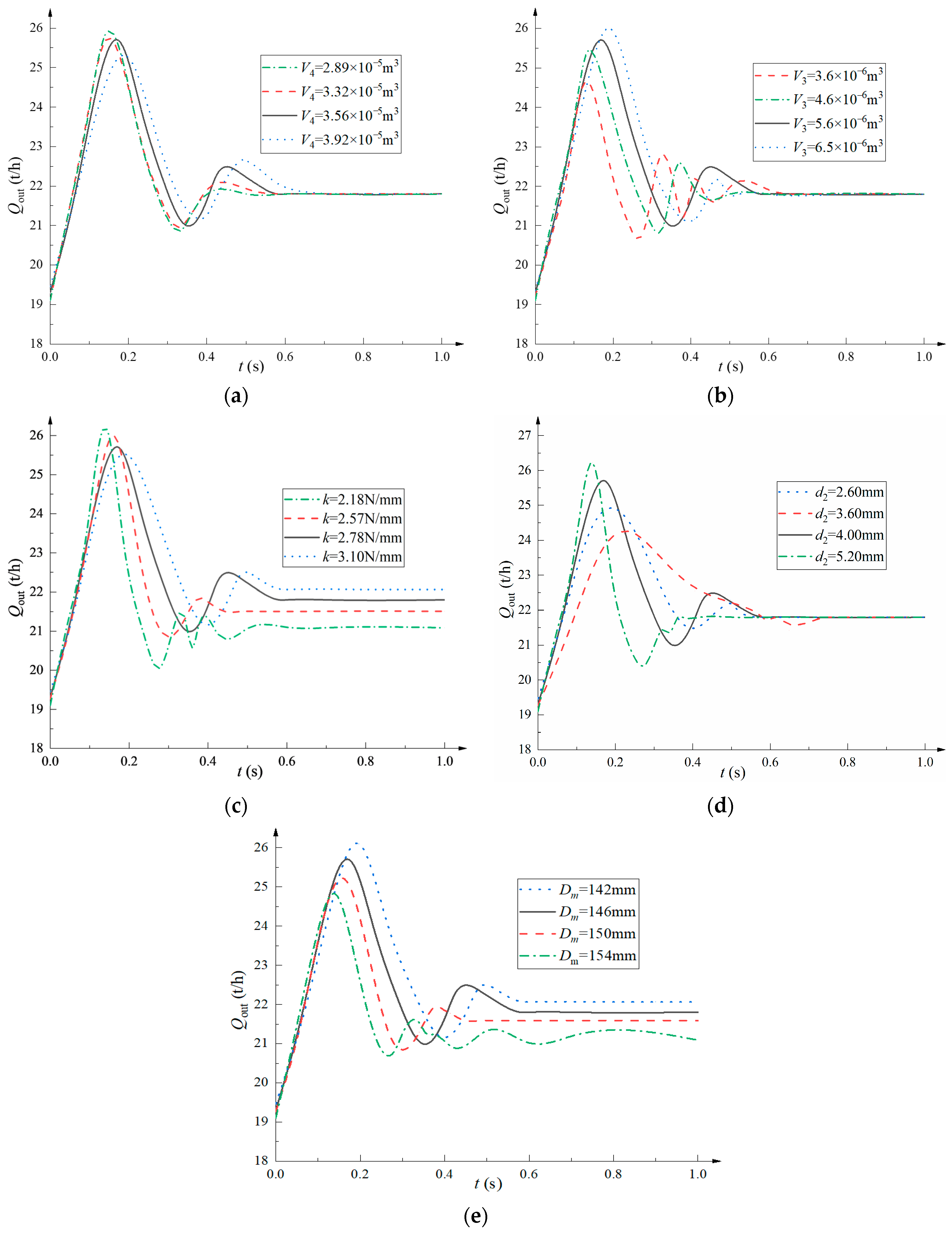
5.1. Influence of Each Structural Parameter on Dynamic Characteristics and Control Stability

Take the different diaphragm left volume chamber V₄, diaphragm right volume chamber V₃, spring stiffness coefficient k, pressure guiding hole diameter d₂, and diaphragm outer diameter D_m and obtain the flow dynamic characteristic curve of the balance valve with different structural parameters, as shown in Figure 14. V₄, V₃, and d₂ show a great influence on the overshoot δ and the transition time t_s of the dynamic characteristic curve and show little influence on the residual e. k and D_m show obvious influence on δ and t_s of the dynamic characteristic curve and show a great influence on e, which affects the flow control accuracy after stabilization. The above analysis shows that it is not possible to simultaneously reduce δ, t_s, and e by changing the value of a certain structural parameter. Therefore, the optimization of the balance valve is a multi-objective optimization problem.

5.2. Optimization of Dynamic Flow Balancing Valves with Improved NSGA-II Algorithm

5.2.1. Mathematical Model

Through the analysis of the impact of each structural parameter on the dynamic characteristics, the diaphragm left volume chamber V₄, diaphragm right volume chamber V₃, spring stiffness coefficient k, pressure guiding hole diameter d₂, and diaphragm outer diameter D_m will all have an impact on the transition time t_s, overshoot δ, and residual e of the dynamic characteristic curve. Therefore, x = [k, V₃, V₄, D_m, d₂] is used to represent the independent variable, and the values of transition time t_s, overshoot δ, and residual e are related to the values of k, V₃, V₄, D_m, and d₂, so they can be written as t_s(x), δ(x), and e(x). The good dynamic characteristics of the balance valve mean that t_s(x), δ(x), and e(x) should be as small as possible, so the optimization objective can be written as min: t_s(x), δ(x), and e(x). The overall optimization model of the dynamic characteristics of the balance valve can be written as:

$$\{\begin{array}{l}find:x={\left[k,V_3,V_4,D_m,d\right]}^T\\ min:t_s\left(x\right),\delta \left(x\right),e\left(x\right)\\ 2.0 \mathrm{N}/\mathrm{m}\mathrm{m}\le k\le 3.3 \mathrm{N}/\mathrm{m}\mathrm{m}\\ 3.2\times {10}^{-6} {\mathrm{m}}^3\le V_3\le 6.7\times {10}^{-6} {\mathrm{m}}^3\\ 2.8\times {10}^{-5} {\mathrm{m}}^3\le V_4\le 4.1\times {10}^{-5} {\mathrm{m}}^3\\ 140 \mathrm{m}\mathrm{m}\le D_m\le 156 \mathrm{m}\mathrm{m}\\ 2 \mathrm{m}\mathrm{m}\le d\le 6 \mathrm{m}\mathrm{m}\\ s.t.: 0\le t_s\left(x\right)\le 1\\ 0\le \delta \left(x\right)\le 5\\ 0\le e\left(x\right)\le 3\end{array}$$

(20)

5.2.2. Design of Experiments

The optimal Latin hypercube experimental design method can reduce the number of sample points on the premise of ensuring uniform filling of the design space and greatly reduce the computational cost. Through the optimal Latin hypercube experimental design, the design variables selected for the dynamic flow balance valve structure are experimentally designed, 100 sample points are extracted, and the response value of each sample point is calculated through the co-simulation method.

5.2.3. Combined Surrogate Model Construction

The combined surrogate model, also known as the weighted average proxy model, is based on the principle of neural networks and consists of multiple single surrogate models superimposed in a weighted form. The mathematical expression of the combined surrogate model can be written as [25]:

$$y_{com}(x)={\displaystyle \sum _{i=1}^m{\lambda }_i(x)y_i(x)}$$

(21)

where y_com(x) is the output response of the combined surrogate model; y_i represents the output response of the ith surrogate model; m is the total number of surrogate models; and λ_i is the weight coefficient of the ith surrogate model, and the sum of the weight coefficients λ_i of each surrogate model is equal to 1.

The prediction accuracy of the combined surrogate model depends on the weight coefficients of each surrogate model. In general, a single surrogate model with higher prediction accuracy should be given a larger weight factor, while a surrogate model with a less accurate prediction should be given a relatively smaller weight factor.

Considering the phenomenon that the prediction accuracy of each surrogate model differs greatly under the same problem, the Heuristic calculation method (EG method) is an efficient method for solving the weight coefficient at present [26].

$${\lambda }_i=\frac{{\lambda }_i^{*}}{{\displaystyle \sum _{i=1}^m{\lambda }_i^{*}}}$$

(22)

$${\lambda }_i^{*}={\left(E_i+\alpha \overline{E}\right)}^{\beta } \alpha <0, \beta <0$$

(23)

$$E_i=GMS{E}_i$$

(24)

$$\overline{E}=\frac{{\displaystyle \sum _{i=1}^m{E}_i}}{m}$$

(25)

where α represents the importance of the average value of GMSE; and β represents the importance of each single surrogate model accuracy index. When α = 0.05 and β = −1, the combined surrogate model and prediction have higher accuracy and the best stability.

According to the different response values of the dynamic characteristic curve of the balance valve, the optimal weight coefficients of every single surrogate model in the combined surrogate model can be solved according to Equations (17)–(20), as shown in Table 1.

Firstly, the RSM, RBF, and Kriging surrogate models of the dynamic characteristics of the dynamic flow balancing valve are established, respectively, and the R² value of the proxy model is obtained, as shown in the Figure 17. It is found that the R² value of the surrogate model constructed by RSM and RBF is closer to 1 and has higher fitting accuracy. Therefore, combining RSM and RBF builds a surrogate model with higher accuracy.

According to the weight coefficients of every single surrogate model in

Table 2. Single surrogate model weight coefficients.

Output Response	Weight Factor
	RSM	RBF
Δ	0.5040	0.4960
ts	0.4391	0.5609
E	0.4516	0.5484

, a combined surrogate model of each performance parameter of the dynamic flow balance valve is constructed. The three-dimensional surface of the combined surrogate model of the performance parameter δ is shown in Figure 17, and the three-dimensional surface of t_s and e will not be shown due to space limitations.

The fitting effect diagram of each output response of the combined surrogate model of δ is shown in Figure 18a–c. The coefficients of determination R² for output responses δ, t_s, and e are 0.9724, 0.9703, and 0.9824, respectively. As can be seen from Figure 19, the R² of the combined surrogate model is closer to 1, and the prediction accuracy is higher than that of the RBF neural network surrogate model, RSM surrogate model, and Kriging surrogate model, so the combined surrogate model can be used instead in co-simulation to optimize the design.

5.2.4. Optimization of Valve Based on Improved NSGA-II

When the classical NSGA-II algorithm solves the multi-objective optimization problem with three or more optimization objectives, its optimization efficiency is low due to the deficiency of the dominance relationship, and it is not easy to converge to the Pareto frontier. The optimization problem of the balance valve is a three-objective optimization, so it is necessary to introduce the improvement method of the relevant non-dominant relationship. To solve the shortcomings of the existing dominance relations in the existing multi-objective optimization algorithms, Tian et al. [27] propose a strengthening dominance relation (SDR) processing method that can be used to solve multi-objective optimization problems greater than or equal to three dimensions. In the niche of each local area, SDR can retain the solution with the best convergence as a non-dominated solution, and SDR does not contain any parameters that need to be set manually. The SDR is embedded in the non-dominated processing program module of the NSGA-II algorithm to construct an improved NSGA-II multi-objective optimization algorithm. The algorithm flow is shown in Figure 20.

The optimal solution set obtained by the NSGA-II algorithm is shown in Figure 21. The minimum overshoot solution A, the shortest transition time solution B, the minimum residual solution C, the pre-optimization solution, and the final optimization solution are shown in

Table 3. NSGA-II solution results.

Case	Structural Parameters					Response Value
	k (N/mm)	V3 (m3)	V4 (m3)	Dm (mm)	d (mm)	δ (t/h)	ts (s)	e (t/h)
A	2.35	5.31 × 10−6	3.39 × 10−5	151.7	3.4	3.52	575	1.61
B	2.21	4.96 × 10−6	3.28 × 10−5	153.8	3.2	4.12	563	1.38
C	2.69	3.93 × 10−6	2.96 × 10−5	147.2	4.5	5.49	363	2.13
initialization	2.78	5.60 × 10−6	3.56 × 10−5	146.0	4.0	4.16	570	2.39
optimization	2.32	4.60 × 10−6	3.19 × 10−5	151.3	3.7	4.03	451	1.81

. The minimum overshoot value in scheme A is 3.52 t/h, the minimum residual difference in scheme B is 1.38 t/h, and the shortest transition time in scheme C is 363 ms. The overshoot of the comprehensive optimal solution is 4.03 t/h, the transition time is 451 ms, and the residual is 1.8 t/h.

The optimal solution set obtained by the improved NSGA-II algorithm with SDR processing is shown in Figure 22. The minimum overshoot solution A, the shortest transition time solution B, the minimum residual solution C, the pre-optimization solution, and the final optimization solution are shown in

Table 4. Improved NSGA-II solution results.

Case	Structural Parameters					Response Value
	k (N/mm)	V3 (m3)	V4 (m3)	Dm (mm)	D (mm)	Δ (t/h)	ts (s)	e (t/h)
A	2.32	5.28 × 10−6	3.41 × 10−5	151.5	3.3	3.13	558	1.57
B	2.18	4.89 × 10−6	3.23 × 10−5	154.1	3.1	3.69	559	1.32
C	2.61	3.92 × 10−6	2.93 × 10−5	147.0	4.5	5.16	352	2.09
initialization	2.78	5.60 × 10−6	3.56 × 10−5	146.0	4.0	4.16	570	2.39
optimization	2.30	4.52 × 10−6	3.11 × 10−5	151.6	3.6	3.86	427	1.65

. The minimum overshoot value in scheme A is 3.13 t/h, the minimum residual difference in scheme B is 1.32 t/h, and the shortest transition time in scheme C is 352 ms. The overshoot of the comprehensive optimal solution is 3.86 t/h, the transition time is 418 ms, and the residual is 1.65 t/h.

Comparing the solution sets, we can see that the improved NSGA-II algorithm can better converge to the Pareto frontier than the NSGA-II algorithm. The minimum overshoot solution A scheme, the shortest transition time solution B scheme, the minimum residual error solution C scheme, and the comprehensive optimization scheme of the improved NSGA-Ⅱ algorithm are all better than the NSGA-Ⅱ algorithm.

Based on the MATLAB/Simulink–FLUENT/UDF co-simulation model, the dynamic characteristics and flow control accuracy of the optimized valve are simulated and compared with the data before optimization, as shown in Figure 23. The transition time of the dynamic characteristic curve is reduced from 570 to 431 ms; the overshoot is reduced from 4.16 to 3.83 t/h; and the residual is reduced from 2.39 to 1.63 t/h. To sum up, the dynamic characteristics of the dynamic flow balance valve after optimization are better than those before optimization, and the discrepancy of the stable flow from the center of 20 t/h is small.

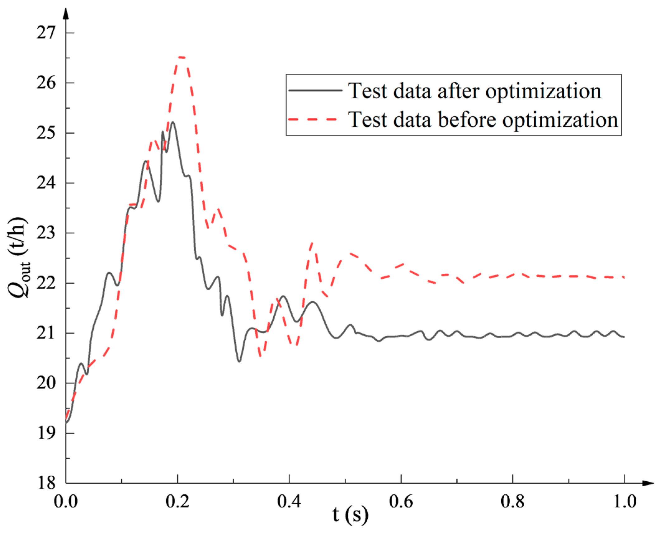
5.3. Experiment to Verify the Optimization Effect

The dynamic characteristics of the optimized valve are tested, and the results are shown in Figure 24. The maximum flow value of the flow dynamic characteristic curve is 25.13 t/h, the transition time is 0.506 s, the flow rate is finally stabilized at 20.87 t/h, and the dynamic adjustment performance has been greatly improved. The experimental results verify that the improved NSGA-II algorithm has a better optimization effect.

6. Conclusions

In this paper, a high-precision co-simulation modeling method for dynamic flow balance valve is proposed, and the valve is optimized by combining the combined surrogate model and improved NSGA-Ⅱ algorithm. The specific conclusions can be summarized as follows:

1. To solve the problem of the low accuracy of the current dynamic flow balance valve simulation method, a co-simulation model combining MATLAB/Simulink and the UDF dynamic grid is established. Comparing the simulation results with the test data, it can be concluded that the relative discrepancy between the simulation results and test data does not exceed 5%; it is far superior to the 8%~10% discrepancy of the existing self-operated valve dynamic characteristic numerical simulation method. Therefore, the co-simulation method proposed can provide a numerical simulation basis for the development of high-precision dynamic flow balance valves.

2. The volume of the left and right chambers of the diaphragm and the diameter of the pressure-impressing hole have obvious effects on the overshoot and transition time of the dynamic characteristic curve but show little effect on the stable flow value. The spring stiffness and outer diameter of the diaphragm also have a significant impact on the overshoot and transition time of the dynamic characteristic curve, and the spring stiffness and the outer diameter of the diaphragm show a greater impact on the flow control accuracy after stabilization.

3. A weighted proportion composite surrogate model is established that comprehensively considers RSM and RBF. The R² of δ, t_s, and e for this model are 0.9724, 0.9703, and 0.9824, respectively. Compared with the existing surrogate model, the R² of the weighted ratio combined surrogate model is closer to 1 and shows better approximation accuracy.

4. To solve the problem of the poor dynamic performance of the existing dynamic flow balance valve, an improved NSGA-Ⅱ algorithm with the introduction of an enhanced dominance relationship is established, and the key parameters of the dynamic flow balance valve are optimized. After optimization, the dynamic transition time of the valve flow is reduced from 570 to 431 ms, the overshoot is reduced from 4.16 to 3.83 t/h, and the residual is reduced from 2.39 to 1.63 t/h. The optimized valve has been tested, and the results show that the optimized valve shows a good dynamic performance, and the relative discrepancy between the stabilized flow and 20 t/h does not exceed 5%, which can meet the requirements of nearly constant flow.

References

1. Yuan, Y.; Neng, Z.; Haizhu, Z.; Hai, W. A New Model Predictive Control Method for Eliminating Hydraulic Oscillation and Dynamic Hydraulic Imbalance in a Complex Chilled Water System. Energies 2021, 14, 3608. [Google Scholar] [CrossRef]
2. Ran, F.; Gao, D.C.; Zhang, X.; Chen, S. A virtual sensor based self-adjusting control for HVAC fast demand response in commercial buildings towards smart grid applications. Appl. Energy 2020, 269, 115103. [Google Scholar] [CrossRef]
3. Wen, S.; Gao, R.; Guan, H.; Li, H.; Wang, M.; Zhang, S.; Li, A. Air damper with Controlling Capacity Unrelated to duct system resistance. Build. Eng. 2021, 43, 102388. [Google Scholar] [CrossRef]
4. Stobbe, M.; Gerber, A.; Herkel, S.; Réhault, N.; Nytsch-Geusen, C. Information model development for the quality assurance of technical equipment in small buildings. J. Phys. Conf. Ser. 2021, 2042, 012082. [Google Scholar] [CrossRef]
5. Liang, J.; Yang, Q.; Liu, L.; Li, X. Modeling and performance evaluation of shallow ground water heat pumps in Beijing plain. China Build. Energy 2011, 43, 3131–3138. [Google Scholar] [CrossRef]
6. Li, S.; Wu, P.; Cao, L.; She, Y. CFD simulation of dynamic characteristics of a solenoid valve for exhaust gas turbocharger system. Appl. Therm. Eng. 2017, 110, 213–222. [Google Scholar] [CrossRef]
7. Liu, P.; Liu, Y.; Wei, X.; Xin, C.; Sun, Q.; Wu, X. Performance analysis and optimal design based on dynamic characteristics for pressure compensated subsea all-electric valve actuator. Ocean Eng. 2019, 191, 106568–106579. [Google Scholar] [CrossRef]
8. Lei, J.; Tao, J.; Liu, C.; Wu, Y. Flow model and dynamic characteristics of a direct spring loaded poppet relief valve. Proc. Inst. Mech. Eng. Part C J. Mech. Eng. Sci. 2018, 232, 1657–1664. [Google Scholar] [CrossRef]
9. Saha, B.K.; Chattopadhyay, H.; Mandal, P.B.; Gangopadhyay, T. Dynamic simulation of a pressure regulating and shut-off valve. Comput. Fluids 2014, 101, 233–240. [Google Scholar] [CrossRef]
10. Liu, J.; Xie, H.; Hu, L.; Yang, H.; Fu, X. Realization of direct flow control with load pressure compensation on a load control valve applied in overrunning load hydraulic systems. Flow Meas. Instrum. 2017, 53, 261–268. [Google Scholar] [CrossRef]
11. Ye, J.; Zhao, Z.; Cui, J.; Hua, Z.; Peng, W.; Jiang, P. Transient flow behaviors of the check valve with different spool-head angle in high-pressure hydrogen storage systems. Energy Storage 2021, 46, 103761. [Google Scholar] [CrossRef]
12. Zang, J.L.; Yao, H.Y.; Zhang, F.H.; Liu, Z.Y.; Meng, J.; Zhu, J.M.; Wang, Z.M.; Qian, J.Y. Dynamic characteristics analysis of pilot valves with different inlet diameters installed on the main steam valve set. Case Stud. Therm. Eng. 2022, 34, 102004. [Google Scholar] [CrossRef]
13. Zong, C.; Li, Q.; Li, K.; Song, X.; Chen, D.; Li, F.; Wang, X. Computational fluid dynamics analysis and extended adaptive hybrid functions model-based design optimization of an explosion-proof safety valve. Eng. Appl. Comput. Fluid Mech. 2022, 16, 296–315. [Google Scholar] [CrossRef]
14. Tang, W.; Xu, G.; Zhang, S.; Jin, S.; Wang, R. Digital twin-driven mating performance analysis for precision spool valve. Machines 2021, 9, 157. [Google Scholar] [CrossRef]
15. Wang, L.; Zheng, S.; Liu, X.; Xie, H.; Dou, J. Flow resistance optimization of link lever butterfly valve based on combined surrogate model. Struct. Multidiscip. Optim. 2021, 64, 4255–4270. [Google Scholar] [CrossRef]
16. Mao, J.; Yang, L.; Hu, Y.; Liu, K.; Du, J. Research on Vehicle Adaptive Cruise Control Method Based on Fuzzy Model Predictive Control. Machines 2021, 9, 160. [Google Scholar] [CrossRef]
17. Fan, Z.; Li, W.; Cai, X.; Huang, H.; Fang, Y.; You, Y.; Mo, J.; Wei, C.; Goodman, E. An improved epsilon constraint-handling method in MOEA/D for CMOPs with large infeasible regions. Appl. Soft Comput. 2019, 23, 12491–12510. [Google Scholar] [CrossRef] [Green Version]
18. Jiang, R.; Ci, S.; Liu, D.; Cheng, X.; Pan, Z. A hybrid multi-objective optimization method based on NSGA-II algorithm and entropy weighted TOPSIS for lightweight design of dump truck carriage. Machines 2021, 9, 156. [Google Scholar] [CrossRef]
19. Peng, C.; Ouyang, X.; Guo, S.; Zhou, Q.; Yang, H. Numerical analysis of the traction effect on reciprocating seals in the hydraulic actuator. Tribol. Int. 2020, 143, 105966. [Google Scholar] [CrossRef]
20. Wang, N.; Pang, S.; Ye, C.; Fan, T.; Choi, S.B. The friction and wear mechanism of O-rings in magnetorheological damper: Numerical and experimental study. Tribol. Int. 2021, 157, 106898. [Google Scholar] [CrossRef]
21. Qian, J.Y.; Wu, J.Y.; Gao, Z.X.; Wu, A.; Jin, Z.J. Hydrogen decompression analysis by multi-stage Tesla valves for hydrogen fuel cell. Int. J. Hydrogen Energy 2019, 44, 13666–13674. [Google Scholar] [CrossRef]
22. Qian, J.-Y.; Zhang, M.; Lei, L.-N.; Chen, F.-Q.; Chen, L.-L.; Wei, L.; Jin, Z.-J. Mach number analysis on multi-stage perforated plates in high pressure reducing valve. Energy Convers. Manag. 2016, 119, 81–90. [Google Scholar] [CrossRef]
23. Ullah, A.; Amanat, A.; Imran, M.; Gillani, S.S.J.; Kilic, M.; Khan, A. Effect of turbulence modeling on hydrodynamics of a turbulent contact absorber. Chem. Eng. Process.-Process Intensif. 2020, 156, 108101. [Google Scholar] [CrossRef]
24. Küçüktopcu, E.; Cemek, B. Evaluating the influence of turbulence models used in computational fluid dynamics for the prediction of airflows inside poultry houses. Biosyst. Eng. 2019, 183, 1–12. [Google Scholar] [CrossRef]
25. Zhan, D.; Cheng, Y.; Liu, J. Expected Improvement Matrix-Based Infill Criteria for Expensive Multiobjective Optimization. IEEE Trans. Evol. Comput. 2017, 21, 956–975. [Google Scholar] [CrossRef]
26. Segovia, E.; de Vera, G.; Miró, M.; Ramis, J.; Climent, M. Cement mortar cracking under accelerated steel corrosion test: A mechanical and electrochemical model. Electroanal. Chem. 2021, 896, 115222. [Google Scholar] [CrossRef]
27. Tian, Y.; Zhang, X.; Cheng, R.; He, C.; Jin, Y. Guiding Evolutionary Multiobjective Optimization With Generic Front Modeling. IEEE Trans. Cybern. 2018, 50, 1106–1119. [Google Scholar] [CrossRef]
Figure 1. A 3D model of dynamic flow balance valve.
Machines 11 00337 g001
Figure 2. Schematic diagram of the structure of the dynamic flow balancing valve. 1. V-shaped ball core; 2. valve stem; 3. ball valve seat; 4. diaphragm; 5. valve body; 6. regulator valve seat; 7. pressure regulator valve core; 8. O-ring; 9. spring; 10. pressure guiding hole.
Machines 11 00337 g002
Figure 3. Relationship between valve core displacement and rubber diaphragm rebound force.
Machines 11 00337 g003
Figure 4. The principle flow chart of the co-simulation model.
Machines 11 00337 g004
Figure 5. MATLAB/Simulink–FLUENT/UDF co-simulation model.
Machines 11 00337 g005
Figure 6. The division of the flow channel mesh of the valve.
Machines 11 00337 g006
Figure 7. Valve core acceleration dynamic characteristic curve.
Machines 11 00337 g007
Figure 8. Valve core speed dynamic characteristic curve.
Machines 11 00337 g008
Figure 9. Valve core displacement dynamic characteristic curve.
Machines 11 00337 g009
Figure 10. Flow dynamic characteristic curve under different pressure drops.
Machines 11 00337 g010
Figure 11. Pressure field of dynamic flow balance valve. (a) ∆P = 30 kPa, the 0 s moment of the moving mesh. (b) ∆P = 150 kPa, the 0.26 s moment of the moving mesh. (c) ∆P = 270 kPa, the 0.53 s moment of the moving mesh.
Machines 11 00337 g011
Figure 12. Velocity field of dynamic flow balance valve. (a) ∆P = 30 kPa, the 0 s moment of the moving mesh. (b) ∆P = 150 kPa, the 0.26 s moment of the moving mesh. (c) ∆P = 270 kPa, the 0.53 s moment of the moving mesh.
Machines 11 00337 g012
Figure 13. Dynamic flow balance valve spool axial hydrodynamic force. (a) ∆P = 30 kPa, the 0 s moment of the moving mesh. (b) ∆P = 150 kPa, the 0.26 s moment of the moving mesh. (c) ∆P = 270 kPa, the 0.53 s moment of the moving mesh.
Machines 11 00337 g013
Figure 14. Valve flow test and acquisition system. (a) Valve flow test system; (b) valve installed in the test system; (c) electromagnetic flowmeter; (d) pressure drop sensor; (e) test data acquisition system.
Machines 11 00337 g014aMachines 11 00337 g014b
Figure 15. Comparison of dynamic characteristics between co-simulation and experiment.
Machines 11 00337 g015
Figure 16. Flow dynamic characteristics of different structural parameter values. (a) Dynamic characteristic curves of different V4; (b) dynamic characteristic curves of different V3; (c) dynamic characteristic curves of different k; (d) dynamic characteristic curves of different d2; (e) dynamic characteristic curves of different Dm.
Machines 11 00337 g016
Figure 17. R2 value of RSM, RBF, and Kriging surrogate models.
Machines 11 00337 g017
Figure 18. Fitting effect diagram of each output response of the combined surrogate model. (a) Fitting effect diagram of δ; (b) fitting effect diagram of ts; (c) fitting effect diagram of e.
Machines 11 00337 g018aMachines 11 00337 g018b
Figure 19. Coefficient of certainty R2 for each output response for different surrogate models.
Machines 11 00337 g019
Figure 20. Flow chart of improved NSGA-Ⅱ algorithm.
Machines 11 00337 g020
Figure 21. Optimal solution set of NSGA-Ⅱ algorithm.
Machines 11 00337 g021
Figure 22. Improved NSGA-Ⅱ algorithm optimizing solution set.
Machines 11 00337 g022
Figure 23. Comparison of dynamic characteristic curves before and after optimization.
Machines 11 00337 g023
Figure 24. Dynamic characteristics test data of valves before and after optimization.
Machines 11 00337 g024