A Novel Method of Digital Twin-Based Manufacturing Process State Modeling and Incremental Anomaly Detection

Abstract

In the manufacturing process, digital twin technology can provide real-time mapping, prediction, and optimization of the physical manufacturing process in the information world. In order to realize the complete expression and accurate identification of and changes in the real-time state of the manufacturing process, a digital twin framework of incremental learning driven by stream data is proposed. Additionally, a novel method of stream data-driven equipment operation state modeling and incremental anomaly detection is proposed based on the digital twin. Firstly, a hierarchical finite state machine (HFSM) for the manufacturing process was proposed to completely express the manufacturing process state. Secondly, the incremental learning detection method driven by stream data was used to detect the anomaly of the job process data, so as to change the job status in real time. Furthermore, the F1 value and time consumption of the proposed algorithm were compared and analyzed using a general dataset. Finally, the method was applied to the practical case development of a welding manufacturer’s digital twin system. The flexibility of the proposed model is calculated by the quantitative method. The results show that the proposed state modeling and anomaly detection method can help the system realize job state mapping and state change quickly, effectively, and flexibly.

1. Introduction

At present, the demands of manufacturing are characterized by large quantities, individuation, and high complexity, and higher requirements are introduced for the production quality of products [1]. The state of the manufacturing process directly affects the quality of manufactured products. More intelligent manufacturing process management technologies are needed to meet the current demand [2]. These technologies require deep integration of the information world and the physical world to provide fast, real-time, and intelligent decisions for manufacturing processes.

As a new interdisciplinary technology, digital twin (DT) technology has been widely studied because it can provide real-time mapping, prediction, and optimization of the physical manufacturing process in the information world.

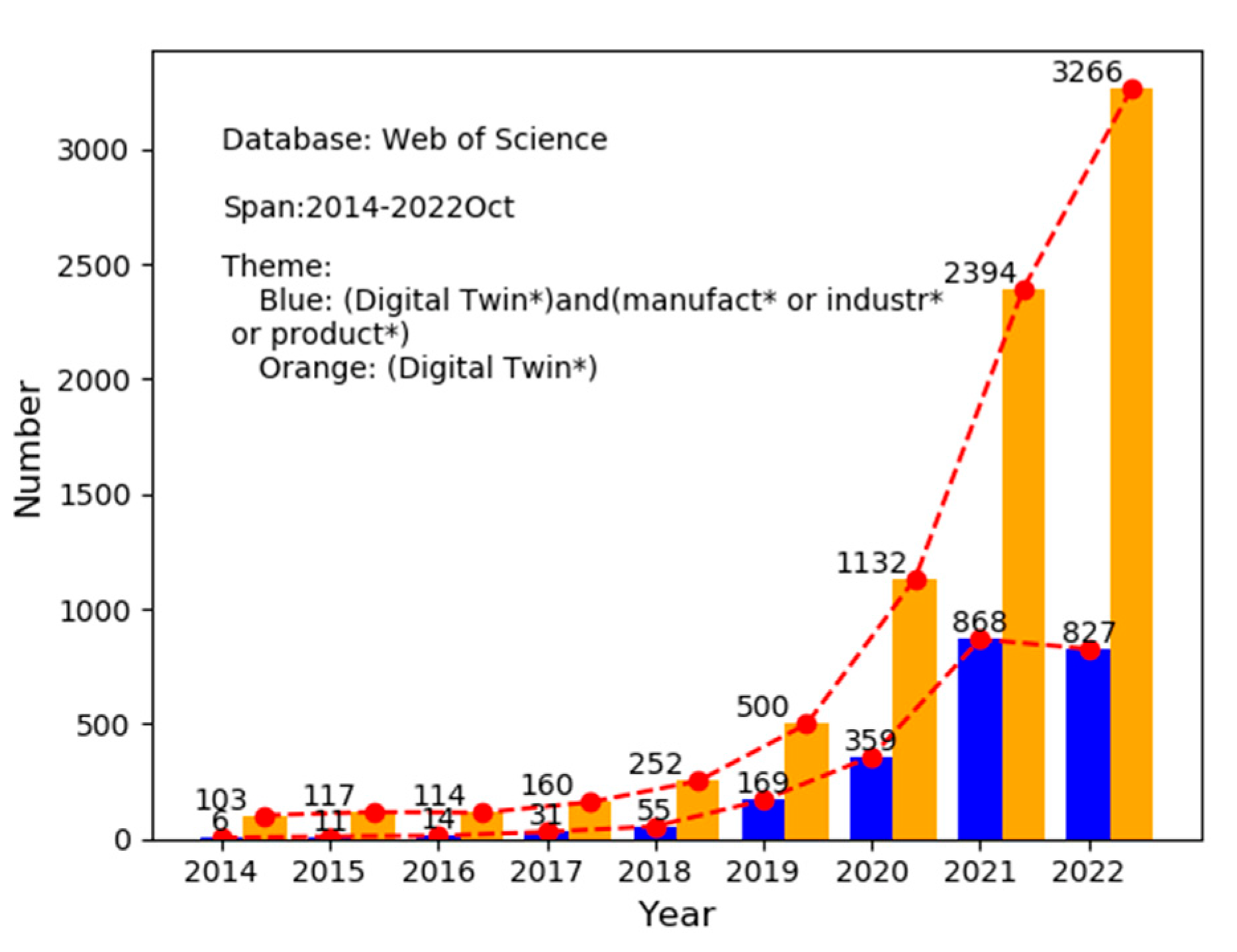
In 2017, Tao Fei [3] elaborated on a new paradigm of a DT-enabled workshop and proposed that the conceptual model of DT is composed of five dimensions, including the physical workshop, virtual workshop, data, service, and connection. The proposal of this five-dimensional model has played a great role in the rapid development of DT in the manufacturing process. As can be seen from Figure 1, DT has attracted wide attention from scholars and developed rapidly after 2017. Moreover, in recent years, scholars have focused on the concept and definition of DT research, gradually more in-depth, to help practical manufacturing research, such as the manufacturing process of maintenance management [4], health monitoring [5], and intelligent control [6].

However, there are two challenges in the management and control of the digital-twin-enabled manufacturing process. (1) The first is the universal characterization of manufacturing process management and control. Due to the individuation and diversity of manufacturing products, the states of various manufacturing equipment in the manufacturing process are also diverse and complex. Universal, flexible, and extensible models are needed to characterize manufacturing processes. (2) The second is mining and the application of manufacturing process flow data. Manufacturing process data present streaming, real-time, and continuous characteristics. It is necessary to mine the flow data in real time and use the flow data to describe the real-time state of the manufacturing process.

Therefore, our major contribution is to propose a general recognition method for digital twin device operation state and incremental recognition based on a real-time streaming data drive. The hierarchical finite state machine is used to express the general operation state of manufacturing equipment in detail and has certain extensibility. In the state machine’s state-change mechanism, an incremental recognition method based on real-time stream data is proposed for anomaly detection.

The remainder of this paper is structured as follows. Section 2 reviews DT-related modeling theory and anomaly detection methods. Section 3 introduces a framework of real-time stream data-driven manufacturing process state modeling and incremental recognition based on DT. The equipment operation state expression based on the hierarchical finite state machine and the incremental anomaly detection method based on real-time stream data in state transformation are introduced in detail in Section 4 and Section 5, respectively. In Section 6, the automatic welding process of a large structural part is taken as an example to introduce the above research method and verify the effectiveness, rationality, and flexibility of the method. Section 7 outlines the summary and prospects of this paper.

2. Literature Review

2.1. Digital Twin Modeling Theory

In 2003, Grieves proposed a prototype of the digital twin named the “Mirror Space Model” [7]. In 2011, Grievous [8] cited the term “Digital twin” in a paper describing product lifecycle management (PLM). In a later paper, he indicated that the conceptual model of DT consists of three dimensions [9], including the entity of the physical space, the virtual entity of the virtual space, and the connection between the physical space and the virtual space.

The National Aeronautics and Space Administration (NASA) collaborated with the U.S. Air Force Laboratory to devise an example of a digital twin vehicle and illustrate the concept of a digital twin vehicle [10]. A digital twin was described as “an integrated multi-physics, multiscale, probabilistic simulation of an as-built vehicle or system that uses the best available physical models, sensor updates, fleet history, etc., to mirror the life of its corresponding flying twin.” Then DT was introduced in “Modeling, simulation, information technology & processing roadmap” released by NASA [11].

From NASA’s definition and the virtual entity of the three-dimensional model proposed by Grieves, it can be seen that DT modeling technology is the core to accurately describing a physical entity and ensuring accurate mapping between the virtual world and the real world [12]. In the process of manufacturing, the premise of real-time monitoring, prediction, and optimization of the manufacturing process is to accurately depict the physical state.

In the process of modeling the physical state, the virtual model of DT is classified into four dimensions: Geometry, physics, behavior, and rules [13]. Among them, the geometric model describes the geometric shape and assembly relationship of the physical entity. The physical model reflects the physical attributes, characteristics, and constraints of the physical entity. The behavior model represents the dynamic behavior of the corresponding internal and external mechanisms of the physical entity. The rule model combines historical data and can use tacit knowledge to make the digital twin more intelligent.

In order to complete the physical representation of the manufacturing process in the information world, the establishment of a high-fidelity digital twin model is very important. Duan [14] proposed a test bed for turbine rotor blades based on a DT. Ma [15] proposed a DT-based workshop management system and Zhuang [16] proposed a DT-based assembly workshop. During the development of a digital twin system (DTS), the mapping between the information world and the physical world is completed. However, the DT model in the above study is relatively static because the model-building process mentioned is only the initial construction of the geometric model.

Schleich [17] proposed a comprehensive reference model based on the skin model shape concept and applied it to the management of geometric variation. This model has certain scalability, interoperability, scalability, and fidelity. Liu [18] proposed a digital twin modeling method based on the bionic principle, which can adaptively construct the dynamic, complex geometric and physical properties of the digital twin model of the machining process. However, while the above digital twin model is adaptive and updatable, it has some defects in speed and accuracy, and the model updating lags behind.

At the same time, scholars have used semantic or knowledge-based methods to build digital twin models. For example, Wang [19] proposed an assembly accuracy analysis method based on the digital twin model of universal parts. The model integrates multi-source heterogeneous geometric models and maps assembly information from assembly semantics to geometric elements. This method realizes the automatic positioning of parts assembly and improves the efficiency of assembly simulation. Gregorio [20] proposed a hybrid virtual product geometry representation method to update the state of the product assembly process. First, they adjusted the geometry of the unassembled component based on knowledge of the geometry of the built component. Bao [21] proposed a method for digital twin modeling of assembly parts. In this method, the ontology is used to define and identify the machining features in advance and obtain the assembly constraint relations, so as to complete the deviation transfer analysis. Liu [22] proposed using the Unified Modeling Language (UML) to build a twin semantic model, which can be used to describe the physical model and behavior model of the physical entity of a large, complex, equipment component test system. Wu [23] proposed a multidisciplinary collaborative design method for complex engineering products based on a digital twin model. A multidisciplinary collaborative design information model of mechanical, electrical, control, and structural complex products based on ontology was established. However, in the above studies, the state mechanism of the manufacturing process was not described in terms of the physical position and geometric shape.

In order to describe the state mechanism of CNC machine tools in detail, Luo [24] established the multi-domain unified modeling method of DT and used the model to diagnose and predict the machine tools’ faults. Wang [25] proposed a digital twin reference model to rotate machinery fault diagnosis and constructed a prototype rotor system to verify the effectiveness of the digital twin model in unbalanced quantification and the fault diagnosis location. Lin [26] used the finite element model as the digital twin model of the full-sized material-compliant wing and used the convolutional neural network to monitor its health. In the above reference, multi-field unified modeling [27], a numerical simulation model [28], etc., were used to construct a digital twin model for specific equipment. However, it was limited to specific devices and specific domains, and cannot be described by state.

2.2. Data Stream Mining Technology

At present, digital twin technology has been applied to solve many problems of intelligent manufacturing, and the artificial intelligence model particularly is used to find defects and identify process anomalies [29].

In the manufacturing process, the anomaly of manufacturing equipment will have a great impact on production and workers. Therefore, many data mining techniques are used for anomaly detection, such as statistics, distance, clustering, or density-based methods [30].

In order to complete the anomaly detection of the process state of manufacturing equipment, the first step is to collect data. The collected data are in an orderly sequence in the form of data or a data block that arrives continuously and rapidly according to the sampling frequency. This sequence is the data stream [31]. Because data streams arrive continuously, the processing times must be as short as possible to provide a real-time response and avoid data queues. In addition to speed, variability is also an important factor in the state transition and real-time decision making of DTs. Variability refers to the non-stationary nature of data, which may change over time, resulting in “conceptual drift”. For example, the non-fault loss of manufacturing equipment in the process of use will make certain changes in the collected data. This requires the model to be updated to offset inaccurate predictions over time.

Kamat [32] proposed a framework composed of an automatic encoder and short-and long-term memory networks for anomaly detection and remaining useful life (RUL) prediction. Calvo [33] proposed an anomaly detection method for an industrial system based on a digital twin ecosystem. Li [34] proposed a DT framework for the analysis of products to be designed based on operational data. Based on this framework, the data are processed and applied to the fault diagnosis of a tunnel excavator. These methods have certain advantages and robustness. However, before the test process, it is necessary to screen the main characteristics and components of multi-source heterogeneous data.

Ensemble learning is a popular method to adapt to the dynamic nature of stream data. The classifier integrates the processing of stream data and helps to adapt to the changes in data characteristics. With respect to data stream mining, ensemble learning can improve predictive ability and flexibly deal with drift problems. Online bagging and boosting [35] is an improvement in the popular ensemble learning method. Bartosz [36] proposed a method to enhance popular online sets by adding waiver options, and to improve the robustness of drift and noise recognition by introducing dynamic and adaptive thresholds to adapt to changes in data streams. Svetlana [37] proposed a TDD-Awareness anomaly detection algorithm that considered the correlation between the sensor data stream and the attributes of each sensor and divided the anomaly detection process into point anomaly and context anomaly, but it had the limitation of time-series prediction.

Tree-based models are suitable for online and incremental learning and have low complexity, low CPU, and low time consumption [38], so they have received extensive attention. The current most popular one is Isolation Forest Algorithms (IForest). Isolating forests is an isolation-based approach that isolates observations by splitting datasets [39]. It consists of two stages, one is the training stage, which builds a forest of random numbers, and the other is the scoring stage, in which the forest provides an abnormal score for each observation in the dataset.

In the early stages, the isolated forest was primarily used for anomaly detection of static data. The Isolation Forest Adapting Stream Data (IForestASD) [40] proposed by Ding was the first to adopt the isolated forest for stream data. In this method, a fixed-length sliding window is used to obtain the stream data, and IForest is used to judge the anomalies of the data in the sliding window. The data for building the tree geometry is sampled, and the changes within the window can be detected based on a predefined threshold for the anomaly rate of all the data within the sliding window. Based on whether the anomaly rate exceeds the predefined threshold, one can determine whether concept drift occurs. Furthermore, in the case of conceptual drift, this results in the retraining of the entire collection based on information on the contents of the current sliding window. IForestASD can be implemented in Scikit-multiflow [41], an open-source ML framework for data streams, and improved in [42]. It is extended by using various drift detection methods, so as to better handle concept drift. Michael Heigl [43] proposed a new pcb-forest framework that can integrate any integrity-based online outlier detection (OD) method to process stream data.

However, the above-mentioned studies all relate to unified flow data without interruption detection and cannot describe changes in the state of manufacturing equipment in real time. In order to describe the state of the manufacturing process, an incremental anomaly detection method based on real-time stream data is proposed.

3. Framework of Incremental Learning Digital Twin System Driven by Streaming Data

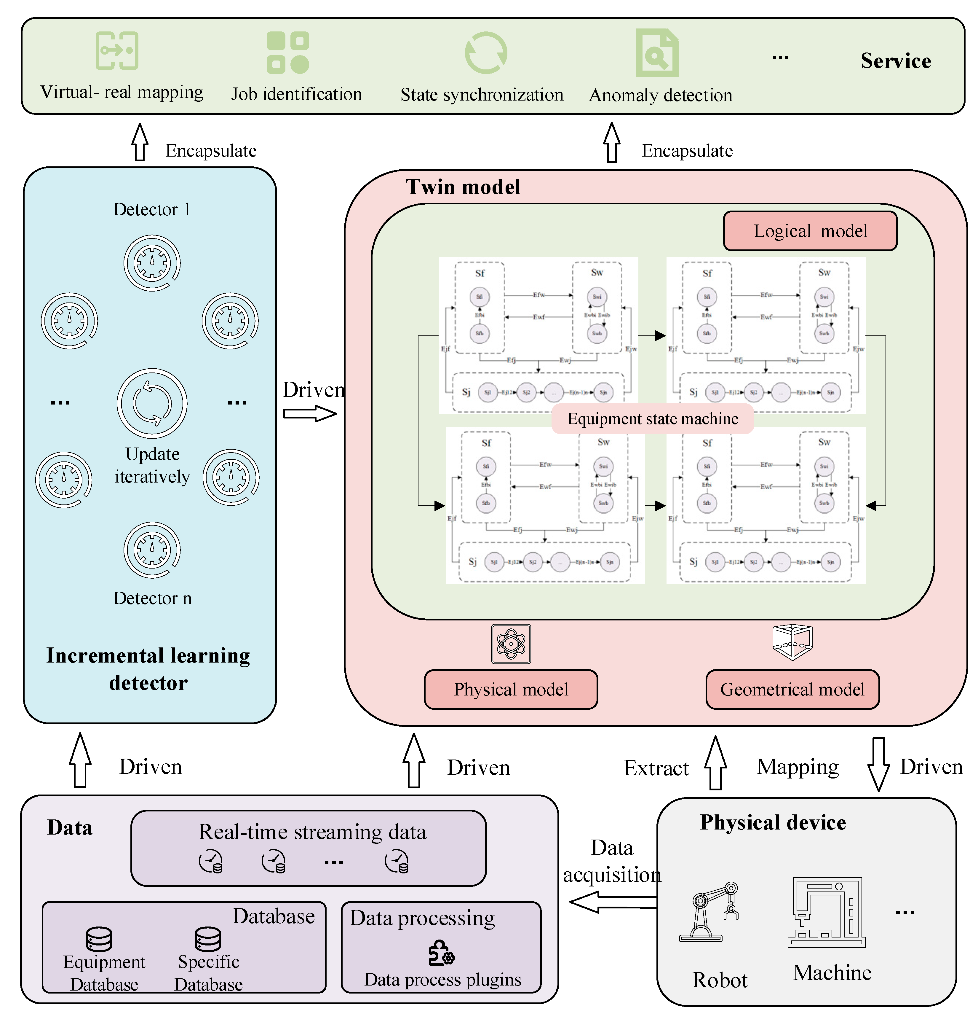
Based on the five-dimensional model established by Tao [3], the framework of an incremental learning digital twin system (IL-DTS) driven by stream data is established, as shown in Figure 2. The framework includes the physical device (Pd), data (D), the twin model (Tm), incremental learning detection (Ild), and service (S).

IL-DTs = {Pd, D, Tm, Ild, S}

(1)

Pd is the sum of the physical hardware of the manufacturing process. Pd includes manufacturing process automation equipment, such as robots, machine tools, and automatic logistics equipment. Pd also includes equipment that supports data acquisition, such as high-precision sensors and a programmable logic controller (PLC). Meanwhile, Pd includes tools used for production fixtures.

D, which can describe the manufacturing process, can be collected through the data-acquisition device contained in the physical device. D includes real-time streaming data, databases, and plugins that contain data processing capabilities. Real-time stream data are data that are continuously input during the manufacturing process. The database includes the device database and other databases, such as the database that records working exceptions and fault types. The data processing plugins include the functions of transmission, cleaning, screening, and dimension reduction of multi-source heterogeneous data, and provide the required data for the database and other DT modules.

Ild is an integrated detector driven by real-time stream data, with the ability to self-update, self-adapt, and self-iterate. It consists of several independent detectors. Each detector should have the ability to process and calculate real-time stream data. In addition, when the characteristics and attributes of stream data change, the detector has the ability to change accordingly. Multiple detectors are integrated to characterize the real state more accurately.

Tm is the mapping model of physical devices in the virtual space, including the logical model, physical model, and geometric model. Geometric and physical models have been described above. The logical model primarily describes the dynamic behavior of physical devices under a specific mechanism and uses Ild to mine the data, and then adaptively updates and drives the dynamic behavior. Finally, the mapping of physical devices will be achieved more intelligently.

S is a set of functions produced by a DTS for manufacturing processes. It is directly oriented to the needs of production and manufacturing. It encapsulates Ild and Tm to realize state synchronization, virtual–real mapping, job identification, and anomaly detection of physical equipment and the manufacturing process.

In summary, the establishment of IL-DTS can be described as follows.

One must process the plugins of D, collect the data of Pd, process the data, and store the data in the database. Ild conducts the initial training of the detector through the database of D, and updates and iterates through real-time stream data. The real-time stream data directly drives the action of the Tm, and Ild drives the state change of the logical model of Tm to complete the state synchronization of Pd. The emergency braking of Pd can also be carried out through anomaly detection and control of the logical model of Tm.

The logical model construction method based on the hierarchical finite state machine (HFSM) method will be introduced in the next section.

4. Logical Model Construction Based on Hierarchical Finite State Machine

The logical model primarily describes the dynamic behavior and state transition of the corresponding elements in the manufacturing process and can cover the required tacit knowledge. Therefore, we construct the logical model through hierarchical finite state machines (HFSMs).

Generally speaking, the manufacturing process (S) can be divided into four states, namely, the waiting state (Sw), blocking state (Sb), fault state (Sf), and job state (Sj). Thus, S can be expressed as S = {Sw, Sb, Sf, Sj}.

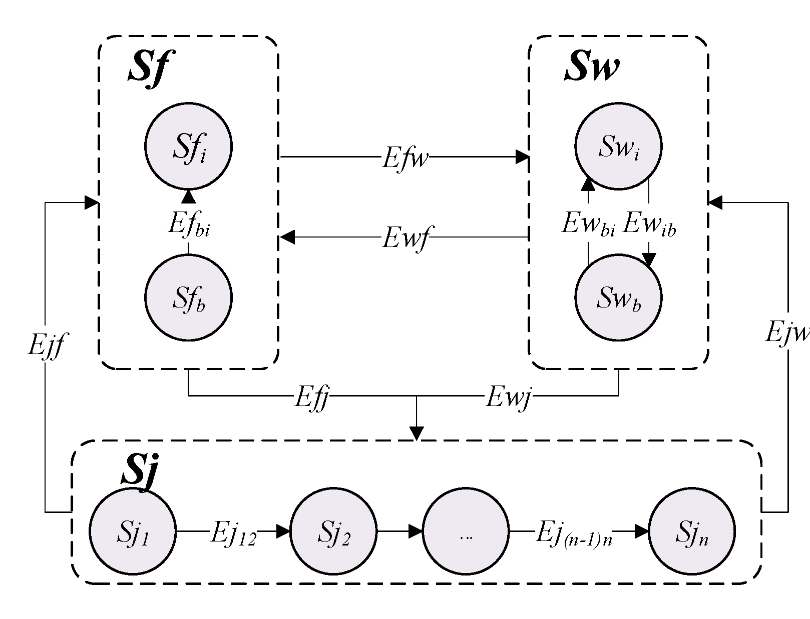
However, the four states cannot express the manufacturing process entirely and in detail. The blocking state is also a type of waiting state. Therefore, the waiting state can be divided into two states, namely, idle waiting (Sw_i) and blocking waiting (Sw_b). Similarly, the fault states can be divided into idle faults (Sf_i) and blocking faults (Sf_b). A blocking fault indicates that the product is in a device and an idle fault indicates that the product is not in a device. In addition to wait states and fault states, the device also contains job states. Job states can be divided into multiple sub-states according to the working procedure. For example, the machine tool needs to process different surfaces in turn. Then the job state of the machine tool can be divided into multiple sub-states according to different surfaces.

Therefore, the operation status of a single device can be described as inner and outer layers, as shown in Figure 3. The state of the outer layer is S = {Sw, Sf, Sj}. Each element of S has its inner layer. Sw = {Sw_i, Sw_b}, Sf = {Sf_i, Sf_b}, and Sj = {Sj₁, Sj₂, …, Sj_n}.

In Figure 3, E_mn represents the job state transition function. E represents the job state transition event, m represents the pre-state, and n represents the post-state.

Table 1. Job state transition event table.

Hierarchy	Job State Transition Function	Specific Meaning
Outer layer	Ejw	Job completion or termination by factors other than failure
	Ewj	The equipment runs properly and meets operating conditions
	Efw	The fault has been removed and no product is in place
	Ewf	An exception occurred
	Ejf	An exception occurred during the job process
	Efj	Exceptions have been removed and the job conditions have been met
Inner layer	Ewbi	The material is released and the device can receive the material normally
	Ewib	The material enters the device and the device has reached its maximum capacity
	Ejpq	The equipment has completed the operation labeled p and met the conditions for starting the operation labeled q.
	Efbi	The material is removed and the fault is not removed

describes the meanings of job state transition.

Based on the Mealy-type finite state machine [44], the equipment operation state model can be represented by six tuples, that is, M = {S, I, O, f, g, S₀} where S is the set of states; I is the finite input set, which represents the state transition event set; O is a finite set of outputs; f is the state transition function, that is, f:S×I→S (for example, f(Sw×E_wj) = Sj indicates that the job status changes from Sw to Sj when the E_wj event is triggered); g is the output function, that is, g:S×I→O (for example, g(S_jm,E_jw)= “Operation m completed”); and S₀ indicates the initial state of the device.

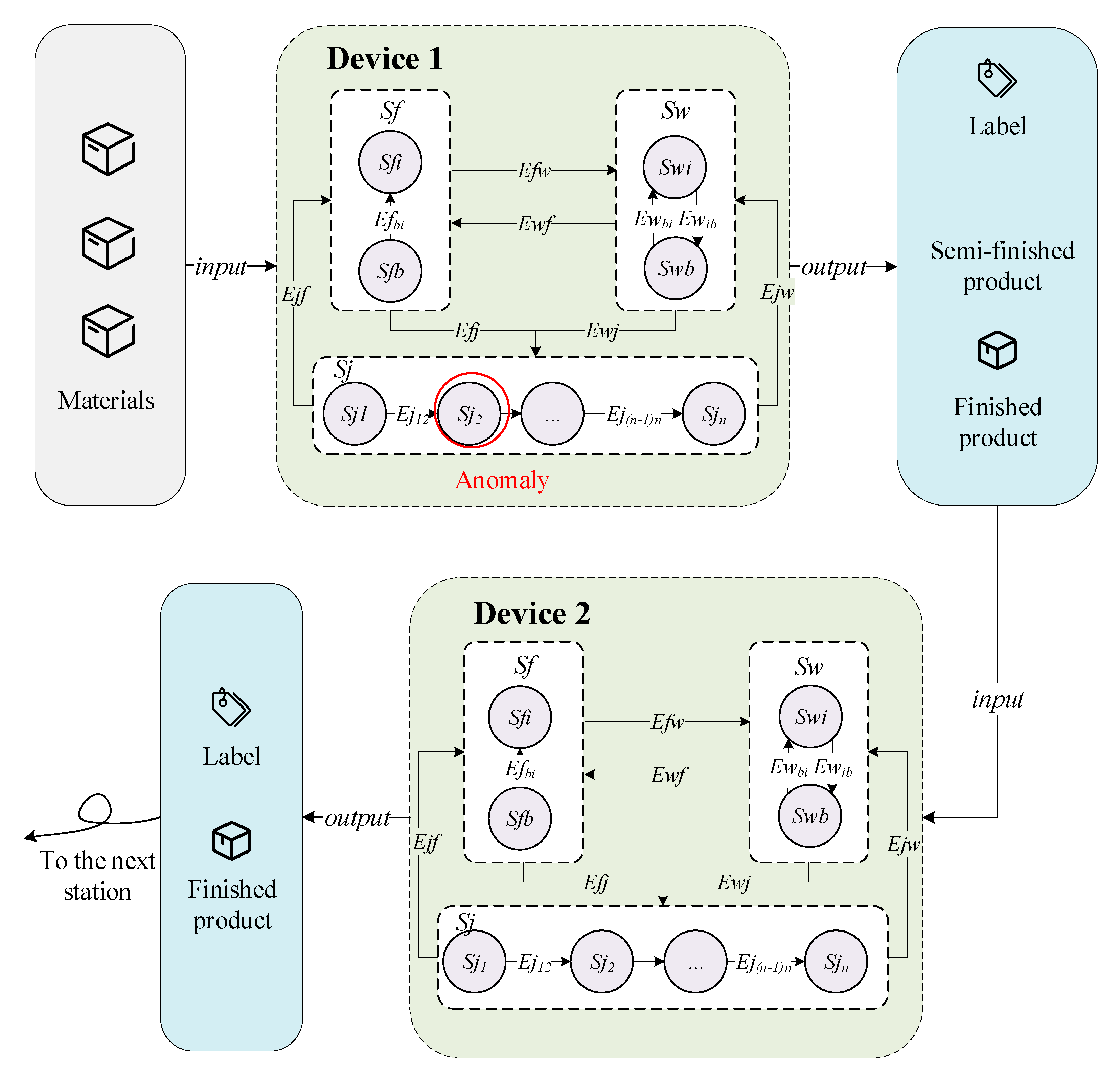
In the initial state, the individual job state of each device can be represented by an HFSM. The device waits for the material to arrive. When Ew_ib is triggered, the device status changes from Sw_i to Sw_b. When E_wj is triggered, the device starts working. In the joint operation of multiple devices, the operation of two devices can be simplified, as shown in Figure 4.

Under normal circumstances, the output of the product after the work state of device 1 is completed with the label “Product completed at device 1”. The label is sent with the product to the required device 2, where the normal operation status is transferred.

However, state machine transitions are slightly different when an anomaly occurs in one of the devices, or when work is transferred to another device for an urgent task adjustment. In Figure 4, E_jf is triggered when an exception for Sj₂ is detected. The state changes to Sf_b and outputs “Sj₂ job interruption of product on device 1”. When the product is removed from device 1, device 1 triggers Ef_bi, and the device state changes from Sf_b to Sf_i. The product is transformed to idle waiting device 2 along with the output label. When the E_wj event is satisfied, device 2 continues the Sj₂ job and the subsequent job process according to the device label. Device replacement may be carried out in accordance with the foregoing in the event of an abnormal or emergency adjustment in the subsequent operation. When the work at this station is completed, that is, Sj_n is completed, the output is “Product completed at device 2”. E_jw transfers to Sw_b. When the product is output in device 2, the state transfers to Sw_i. The product is transferred to the next station with the label.

It can be seen that the state machine can provide an information reference for the device utilization rate, device completion, device failure rate, and can effectively trace the historical information of the product in the manufacturing process. The key to state machine state transformation is to determine whether the working state is abnormal. A method of incremental real-time anomaly detection based on stream data will be introduced in the next section.

5. Incremental Real-Time Anomaly Detection Based on Stream Data

5.1. Algorithm Introduction

Due to the large quantity, rapid, and continuous arrival of manufacturing process data, a digital twinning system needs to adopt a real-time updating anomaly detector to ensure the rapid change of state. 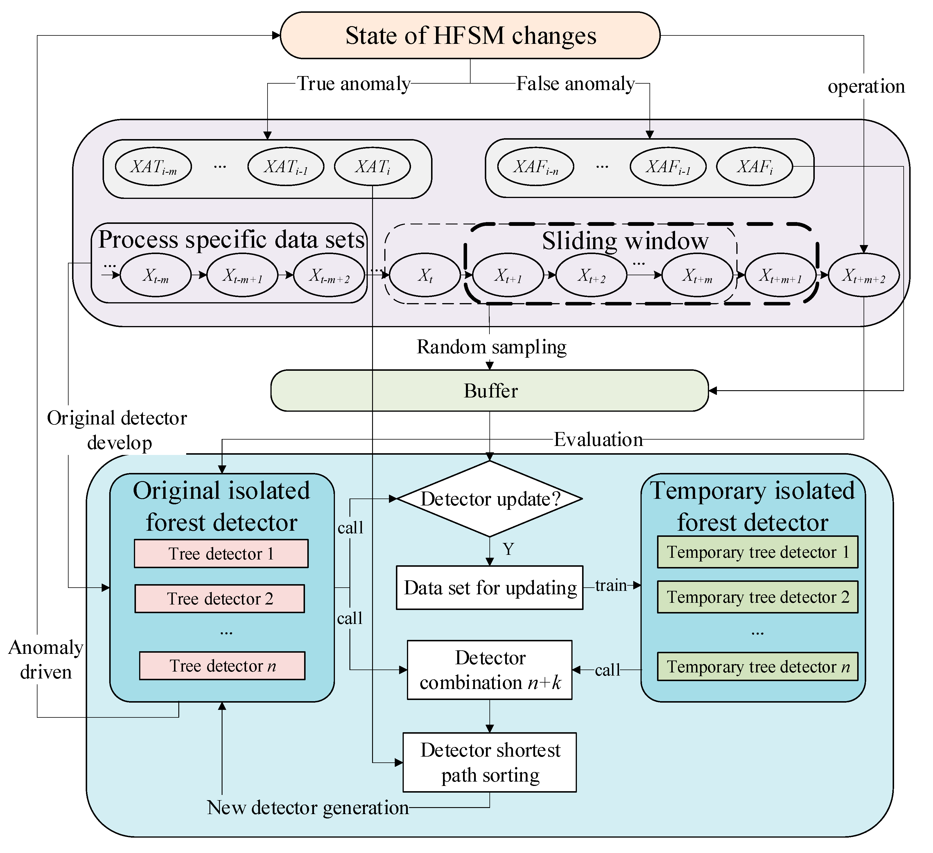Combined with the characteristics of the low complexity and high efficiency of the isolation forest algorithm (IForest) [39], this paper introduces the incremental learning isolation forest real-time anomaly detection method in the state machine, as shown in Figure 5.

Commonly, a working process consists of multiple processes. Therefore, the dataset is also divided into several process datasets according to the process. In a specific process dataset, a detector, including n trees, is built based on IForest. When the operation state enters the specific process, the specific process dataset is selected, and the original IForest detector, sliding window, and buffer are activated.

The newly generated data fill the sliding window in sequence. When the maximum capacity of the sliding window is satisfied, the new data header and tail data are removed. When the job is running, the Bernoulli distribution is used to randomly sample the incoming stream data into the buffer. The original IForest detector was used to detect the anomalies of the incoming stream data. When the data are determined to be an anomaly, the drive state machine changes. The device switches to standby mode and the device state changes to Sf_b. At this time, manual or other intelligent algorithms are used to check the fault. After normal troubleshooting, if it is a real anomaly, the data are regarded as a true anomaly to update the detector. If it is a false anomaly, the data are regarded as a false anomaly (Xaf). Meanwhile, these data are forced to be kept in the buffer.

When the anomaly rate of the sliding window (Rsw) is greater than the anomaly threshold (Rset), it proves that drift may have occurred, so the detector update strategy is triggered. When the buffer is full, the detector is forced to update. However, the above update strategy is different.

When the abnormal rate of the sliding window is greater than the set threshold, the union set comprised of buffer data and sliding window data is used as the training dataset (X) of the update detector. When the buffer is full, the buffer data are used as the training dataset of the update detector, and then the buffer is released. The dataset of the updated detector is used to construct k trees as the new anomaly detector.

The value of k can be obtained using the following equation:

$$k=Rsw\times n$$

(2)

At present, there are n + k new anomaly detectors and original anomaly detectors. The latest true anomaly data (Xat) are extracted and then tested with all current detectors. The shortest paths of the data in all the detectors are calculated and sorted. k detectors with a longer path are eliminated, and n detectors with a shorter path are retained as new detectors.

The pseudocode of the incremental learning isolation forest anomaly detection algorithm in HFSM (ILIForest-HFSM) is as follows (Algorithm 1).

Algorithm 1: ILIForest-HFSM (w, b, n, Rset)

Input: w—sliding window size, b—buffer capacity, n—detector number, Rset—sliding window anomaly threshold Output: new detector W ← W, B ← B ∪ Xaf // Initialize the sliding window and buffer original IForest ← IForest (X, n) // Establish the original IForest detector (n trees) using specific process data X While data comes do Obtain new Xt from the stream W = Update (W, Xt) // Update the sliding window Rsw = Calculate (W,Xlabel) //Calculate the anomaly rate of sliding window Determines whether Xt is added to B based on Bernoulli distribution If Xt is anomaly then Sji changes to Sfb Break If size of B ≥ b then X’ ← B Generate k randomly new IForest ← IForest (X’, k) new IForest ← Update (Xat, new IForest, original IForest) //Among all the detectors, n detectors with the larger shortest path of Xat serve as the new detector end if If Rsw ≥ Rset then X’ ← B ∪ W Generate k randomly new IForest ← IForest (X’, k) original IForest ← Update (Xat, new IForest, original IForest) end if t = t + 1 End while return original IForest

5.2. Experimental Evaluation

In this paper, Smtp, Shuttle, and Forest Cover are the three standard datasets selected to carry out experimental research on ILIforest-HFSM. Basic characteristics of the dataset are shown in

Table 2. Basic characteristics of the data.

Name	Instances	Normal Instances	Anomaly Instances	Attributes	Anomaly Rate
Smtp	95,156	95,126	30	3	0.03%
Forest Cover	286,048	283,301	2747	10	0.96%
Shuttle	49,097	45,586	3511	9	7.15%

.

In this paper, the F value (representing F1 and, running time are used to evaluate the algorithm. The selected sample is not balanced with the actual running process data. The F1 value takes into account both the accuracy rate and the recall rate, so the F1 value is used as an evaluation metric. The F1 value can be calculated as,

$$F1=\frac{2\times precision\times recall}{precision+recall}$$

(3)

A DTS requires real-time performance, so the program’s running time is used as the evaluation metric. In the algorithm proposed in this paper, the variable parameters are the size of the sliding window (W) and the number of detectors (D).

As can be seen from

Table 3. Test result of IForest-HFSM Algorithm.

		ForestCover				Shuttle				Smtp
W	D	F	F’	T	T’	F	F’	T	T’	F	F’	T	T’
50	30	0.12	0.02	67,057	75,470	0.81	0.29	1715	2270	0.13	0.00	3567	5400
50	50	0.12	0.02	79,236	86,357	0.83	0.29	2735	3498	0.13	0.00	5493	7520
50	100	0.12	0.02	101,232	107,919	0.82	0.28	5338	6430	0.13	0.00	10,319	12,328
100	30	0.14	0.02	84,932	91,133	0.83	0.61	3793	3855	0.16	0.00	14,219	14,203
100	50	0.14	0.02	101,126	109,116	0.83	0.60	6037	6249	0.16	0.00	21,432	20,941
100	100	0.15	0.02	148,724	153,292	0.86	0.60	12,136	12,327	0.17	0.00	38,937	36,438
200	30	0.17	0.02	95,306	104,963	0.85	0.71	16,952	16,892	0.18	0.00	20,884	19,679
200	50	0.17	0.02	130,900	140,474	0.89	0.71	25,899	25,724	0.18	0.00	27,841	24,184
200	100	0.17	0.02	212,904	222,475	0.90	0.72	45,056	45,338	0.18	0.00	50,582	43,864

Note. W represents the sliding window size and buffer size, and D represents the number of detectors. F represents the F1 value of ILIForest-HFSM; F’ represents the F1 value of IForest without the state machine. T represents the time consumption of ILIForest-HFSM (second). T’ represents the time consumption of IForest without the state machine (second).

, when the W and D of the two algorithms are the same concurrently, the difference between T and T’ is not large, and the difference primarily comes from the different number of integrator updates and the different total time of training. We will analyze the time later. In ForestCover and Smtp datasets, the improvement effect of F is not obvious compared with that of F’. This is primarily because the sample is extremely unbalanced and there are few anomalies. In addition, the anomaly type of ForestCover is a multi-point continuous anomaly. This causes the sliding window to update the detector at the continuous outlier. As a result, the update of the detector will inevitably lead to the misjudgment of the following normal data. However, in Shuttle data, the F1 value increases significantly, which can prove that the algorithm has certain effectiveness.

When W and D of an algorithm change, it can be seen that F and T increase as W and D increase. It has been proven that when W and D increase, the effect of anomaly detection will also increase. However, it would also lead to a dramatic increase in time consumption. Therefore, we conducted experiments on the original training time and test time of individual data.

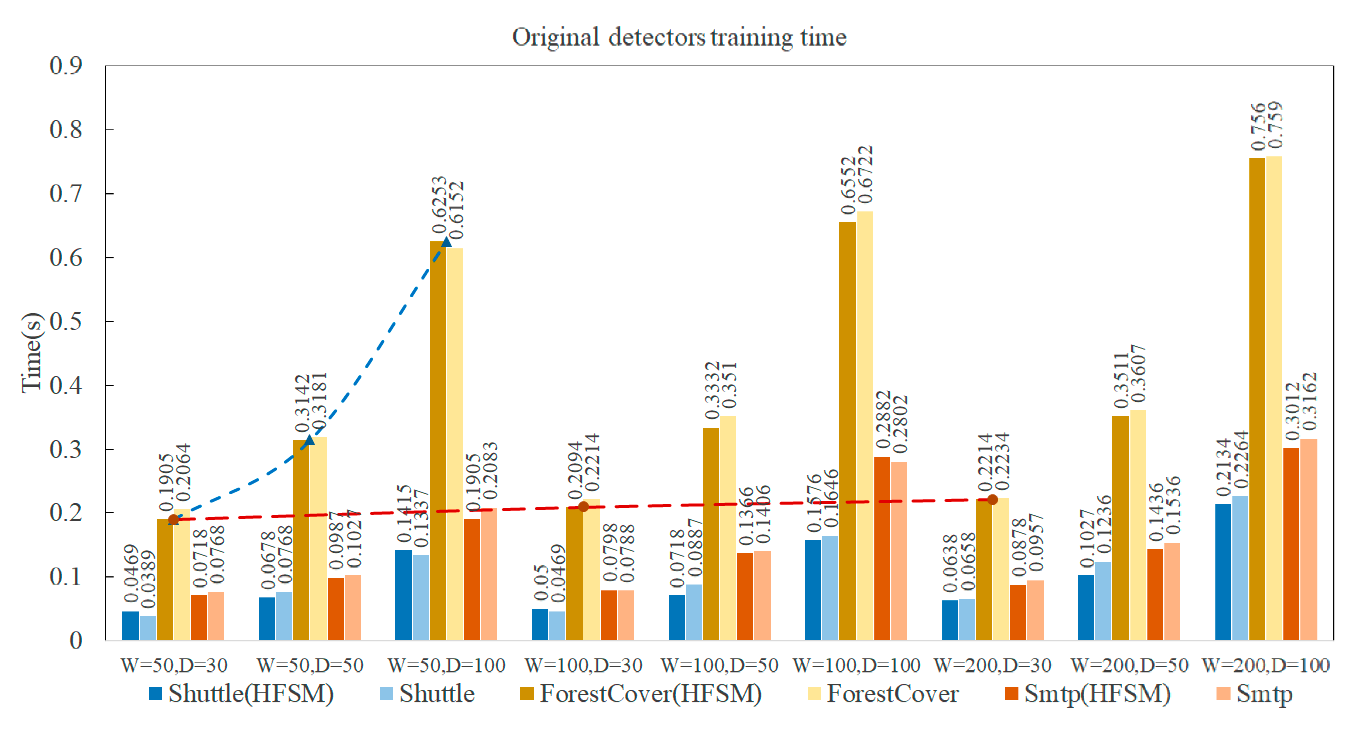
As shown in Figure 6, the dark bars represent the initial detector training time with the IForest-HFSM algorithm, while the light bars represent the initial detector training time without HFSM. When the same training dataset is used, the results are essentially the same when W and D are the same. When W is the same, as D increases, the time becomes longer and longer. When D is the same, as W increases, time increases. However, the broken line in Figure 6 shows that the trend is different. The growth trend when D is the variable is obviously higher than when W is the variable.

When different training datasets are used, the original training time of ForestCover is significantly higher than that of other datasets. The original training time for Smtp is slightly higher than for the Shuttle dataset. This means that the number of original datasets affects the training time of the original detector.

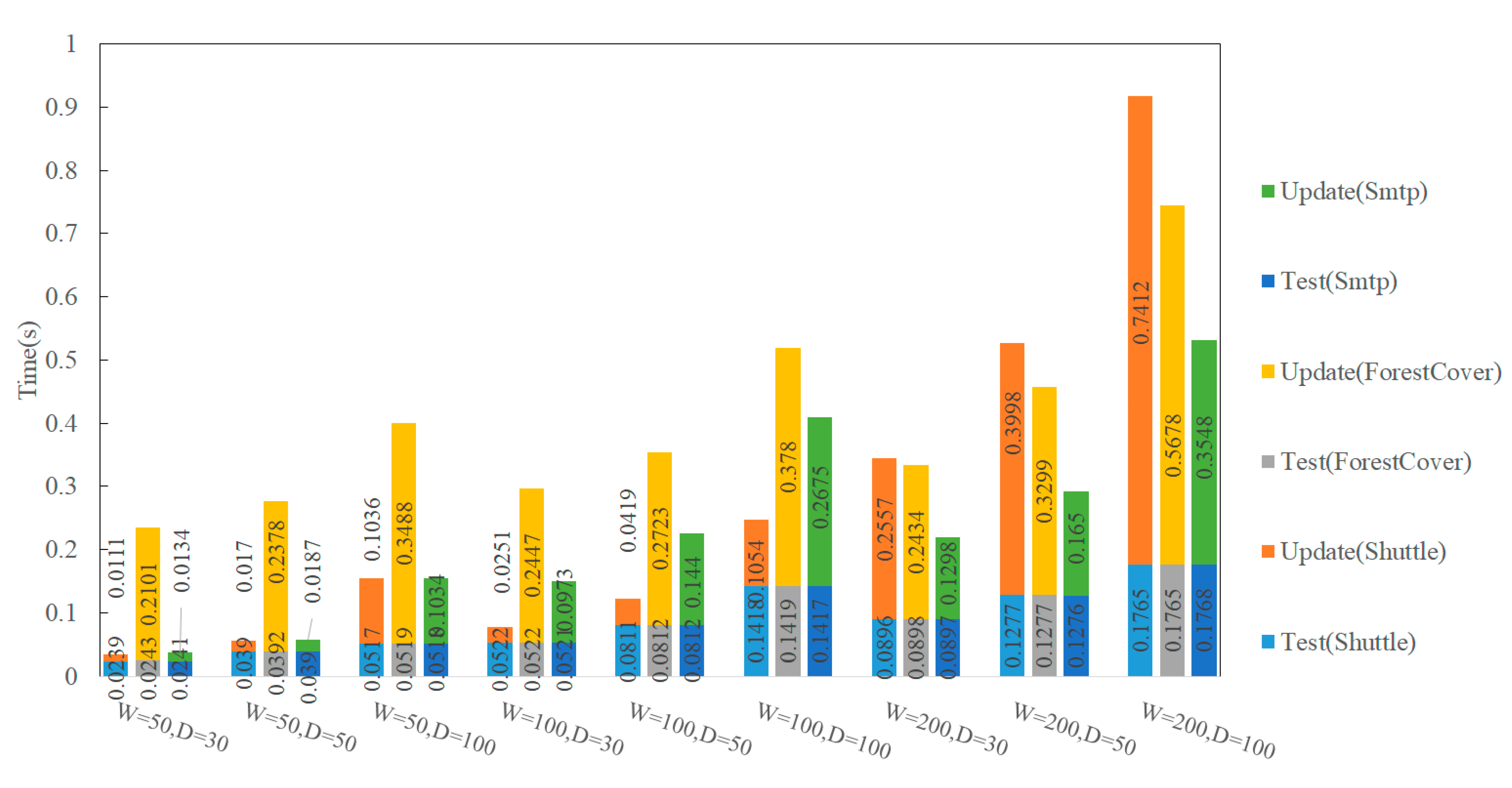
The number of detector updates is different, resulting in different update times for each detector. Therefore, the average update time of each dataset is used to evaluate the algorithm. The total test time for a single dataset is shown in Figure 7.

First, we analyzed the bottom half of the bar chart. In different datasets, when W and D are the same, the time spent on the individual dataset is almost the same. This proves that the test time of an individual dataset is only related to the size of W and D and has nothing to do with the data volume. When W and D increase, the test time increases. When W = 100 and D = 100, the test time of a single dataset exceeds 0.1 s. The test time of W = 200 and D = 30 is close to that of W = 100 and D = 50.

Secondly, we analyzed the top half of the bar chart. In different datasets, when W and D are the same, the average update time of individual datasets varies greatly. This is the result of the proportion of anomalies, data characteristics, and algorithms caused by misjudgment. A too-large proportion of anomalies, continuous anomalies of test data, and excessive misjudgment of the algorithm will force the detector to update, which increases the time and resource consumption of the algorithm update. When W and D increase, the average update time of individual datasets also increases. This is because updated data of the detector comes from the sliding window. The number of detector updates is related to the number of detectors and the update rate.

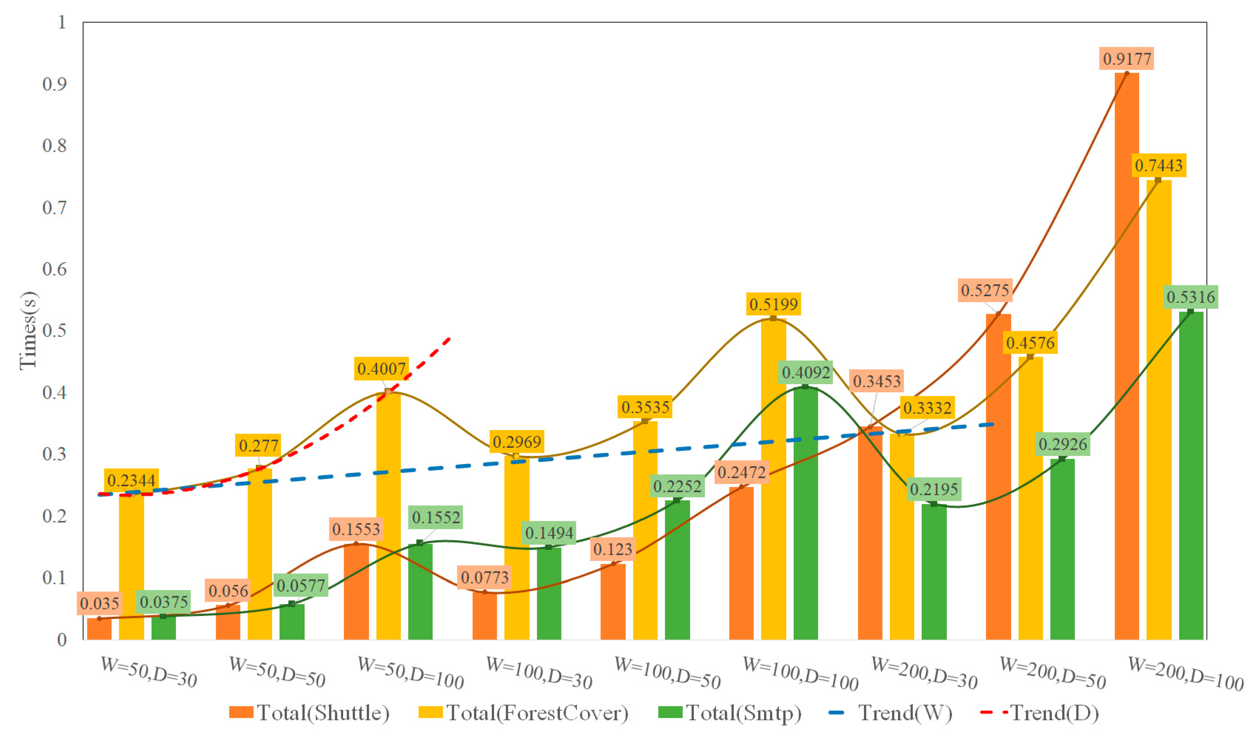
To further illustrate the time consumption of each dataset, we compare the trend when W changes with that when D changes, as shown in Figure 8.

The lines in Figure 8 indicate that when D = 30, the total time is at the bottom, and the minimum value is taken. When D is constant, the total time of an individual dataset increases linearly as W increases, as shown by the blue dashed line in Figure 8. When W is constant, the total time of individual datasets grows exponentially as D increases, as shown by the red dotted line in Figure 8. Time resource consumption increases significantly with the increase in D. With W = 200 and D = 100, the total test time of an individual dataset reaches 0.9177 s. This is obviously not sufficient for real-time effects. Combined with Table 3, when W is the same, the F1 value does not increase significantly with the increase in D. Therefore, it is recommended to use W = 100 and D = 30. The results of the test in the three datasets are the best.

6. Case Study

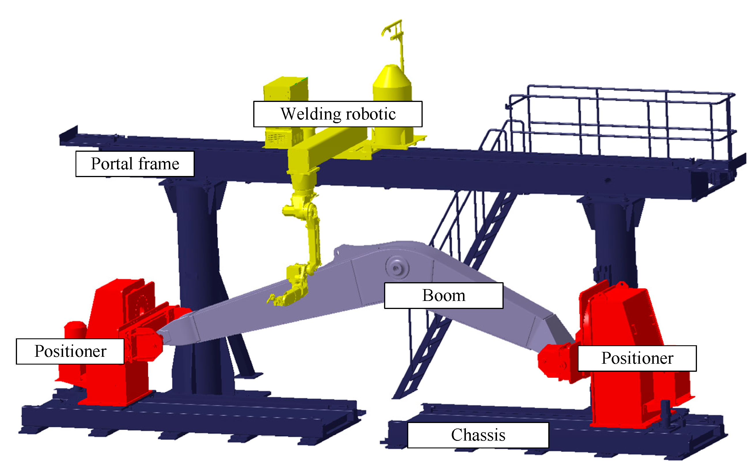
Taking a robot welding workstation of a large equipment manufacturer as an example, this paper introduces DTs based on the aforementioned method. The welding workstation is composed of a welding robot, gantry frame, positioner, and chassis, as shown in Figure 9. Its main task is to weld the boom body of large excavating machinery.

The equal-scale geometric model of the robot workstation is constructed using Catia. The calibration of the initial position, constraint relationship, and parent–child hierarchical relationship of the device is completed in Catia. 3DsMax software imported the stp file generated by Catia, carried out coloring, material addition, and environment construction of the model, and completed the property construction of the physical model. Finally, the exported FBX file was imported into Unity3D to carry out the main development process.

Because the automatic welding process can be divided into multiple tasks according to the weld seam, the tasks can be represented as J1, J2,…, J16. Therefore, according to the above state machine, the hierarchical finite state machine of a single station of robot work is implemented in Unity.

The real-time IOT platform of the enterprise is selected for data collection, and JSON data are accessed through the API interface, as shown in

Table 4. Data acquisition table of robot welding workstation.

Category	Specific Data (Type)
Process data	Welding current (float)
	Welding voltage (float)
	Wire feed speed (float)
Automatic data	Robot joint J1-J6 Angle (float)
	Truss position of robot (float)
	Angle of positioner (float)

.

The sampling frequency of the data obtained through API is 0.5. Linear interpolation is used to interpolate the data and complete the mapping of the twin model in the virtual space. During the test, approximately 2% of the training data were abnormal compared to normal. The initial parameters of the anomaly detector are set as follows. The sliding window size was set to 100, the number of integrators was set to 30, the time for integrator testing of each dataset was approximately 0.08 s, which met the updating frequency, and the accuracy rate reached more than 95%.

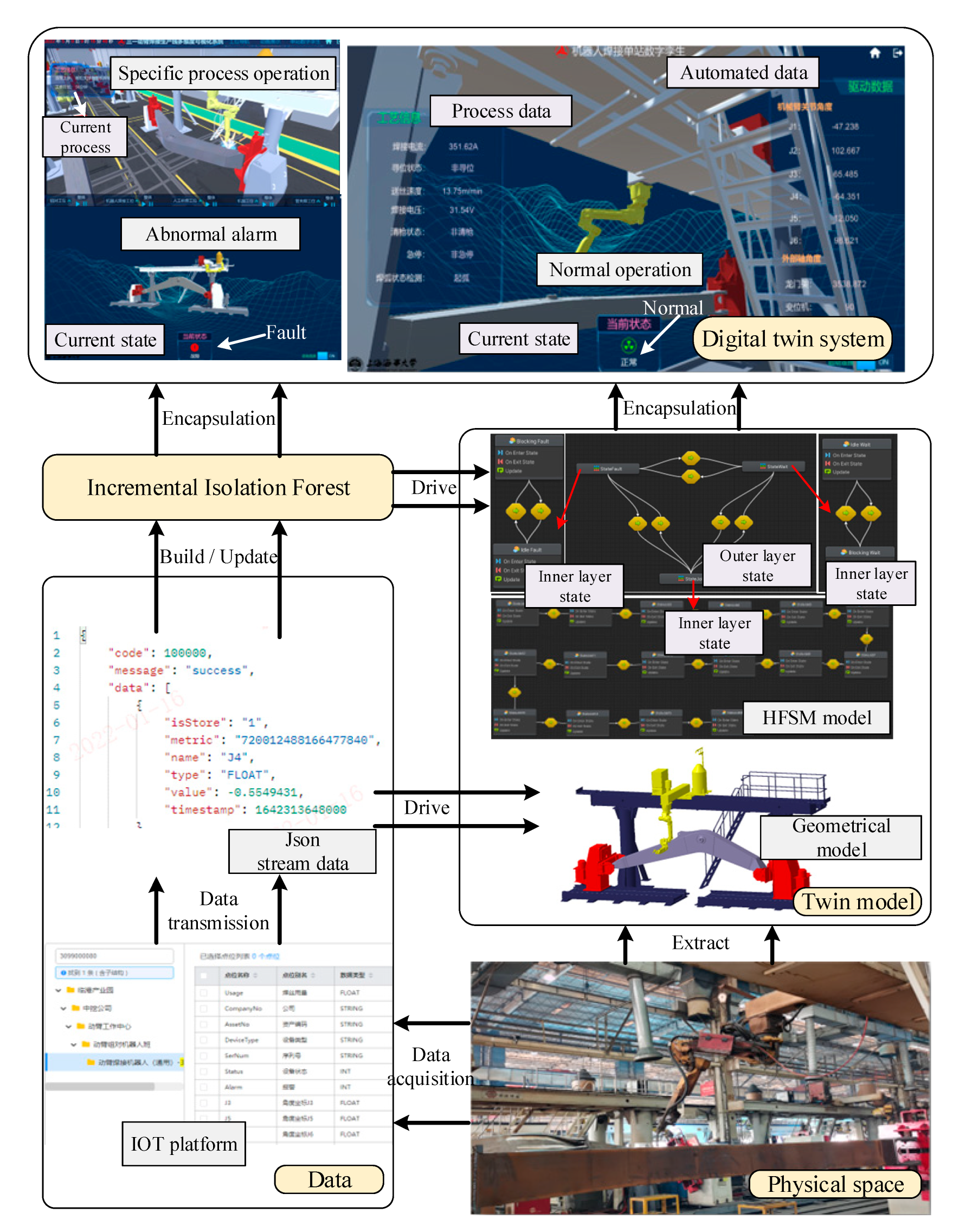
The specific implementation of the digital twin system is shown in Figure 10.

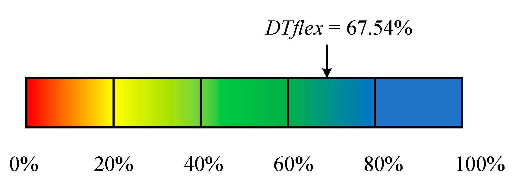
In order to quantitatively evaluate the proposed DT model, we used the method for measuring flexibility proposed by Psarommatis [45] to evaluate the flexibility of the DT model. The flexibility of the model proposed in this paper (DTflex) can be derived from

Table 5. DTflex measurement with method proposed by Psarommatis [39].

QNo.	Answer	Explanation
Q1	Yes: +0.8	The method can be used unchanged under any circumstances. There are six input parameters: Slide window size, buffer size, number of detector trees, number of nodes per tree, update threshold, and input stream data.
Q2	Specific: −0.5	The method is based on experimental design, so it needs to perform specific experiments to obtain the data necessary to train the DT model.
Q3	Yes: +0.6	When using different datasets, the method can increase the dataset or increase the characteristic parameters.
Q3.1	Yes: −0.2	Although datasets or characteristic parameters are available, the data selected depend on the number of integrator trees.
Q3.2	No: +0.1	Data original training depends on the number of detector trees and the number of forests. The number of training sessions does not change as a result.
Q3.3	No: +0.2	Similarly, the model does not change.
Q3.4	No: +0.2	The output parameters are not affected by changes in the input parameters.
Q4	Yes: +0.4	Input datasets or characteristic parameters can be decreased.
Q4.1	No: +0.2	Decreasing the input does not affect the DT model. The only issue is that with fewer input parameters, the accuracy of the model will be lower.
Q4.2	No: +0.2	Some parameters can be set to default values, with reduced accuracy.
Q5	Yes: −0.6	The method can update the detectors in the process of outputting anomaly detection.
Q6	Yes: +0.5	The output results of multiple detector trees can be processed in other forms to generate new output parameters.
Q6.1	No: +0.2	No limitations on increasing the number of output parameters.
Q7	Yes: +0.8	When the external data change, the DT model can adapt to change.
Q8	Yes: +0.3	The DT model is a simple mathematical model that can be run on any computer.
Q9	Yes: −0.3	This method requires training at the beginning, but the training time is acceptable.
$\mathrm{Total} \mathrm{flexibility} \mathrm{of} \mathrm{the} \mathrm{DT} \mathrm{methodology} DTflex=4.8+\sum Q_j=7.7$$, 0<DTflex\le 11.4$

.

We converted DTflex to a percentage and were able to obtain DTflex = 67.54%. Figure 11 illustrates this result. It can be seen that the algorithm has good flexibility.

Over the course of the experiments and the case study, the mentioned hierarchical finite state machine represented the state of each manufacturing device very quickly, and it could be rapidly reconstructed and extended according to the manufacturing task.

In the mentioned algorithm, when W = 128 is used, the maximum number of nodes is 255. The maximum length of nodes is b bytes, and D is the number of trees. Therefore, the working model for real-time anomaly detection is less than 255Db bytes. This is trivial for the loading of 3D models of manufacturing processes. The time complexity in the original training phase is O(nDlogW). The time complexity of the individual dataset test evaluation process is O(DlogW) and the time complexity of the model update process is O(WDlogW + D²). It can be seen that the proposed digital twin method has a fast convergence speed and a small integration scale, and can monitor anomalies efficiently and quickly in real time.

In addition, when W = 100 and D = 30, the average test time of an individual dataset is lower than 0.1 s under the Shuttle dataset and the current case dataset. It is possible to service the current digital twin system, and it can be effectively and flexibly deployed in the digital twin system of the manufacturing process.

7. Conclusions

This paper proposed a method of digital-twin-based manufacturing process state modeling and incremental anomaly detection. (1) A framework of incremental learning digital twin system was proposed, and the incremental learning detector was added as a new layer to the existing digital twinning framework. (2) A manufacturing process modeling method based on a hierarchical finite state machine was introduced. By introducing a single-device running state model and a multi-device running state model, the universality of the manufacturing process running state model was realized. (3) An incremental isolation forest detector driven by stream data was introduced. The algorithm can quickly and effectively identify anomalies within the manufacturing process and make changes to the manufacturing process. (4) The incremental learning digital twinning system driven by stream data was introduced via the boom welding workstation.

The paper is primarily concerned with the anomaly detection of the state machine from the working state of a process to the fault state and does not involve the classification of the fault state. However, the description of fault states in the proposed state model is extensible. In addition, the real-time performance of the current algorithm does not reach the optimal state. To be exact, the current algorithm only achieves quasi-real-time performance. In order to further improve the accuracy, greater time loss reduces the real-time performance. According to the characteristics and changing trends of current stream data, it is very necessary to reduce the time for anomaly detection or to predict the anomalies that will occur. Therefore, future work will primarily focus on the improvement of the state machine model, the enhancement of anomaly detection efficiency of the algorithm, and the early warning of real-time stream data.