Wear of Abrasive Tools during CMC Machining

Abstract

Machining CMCs under productivity conditions while limiting tool wear and material damage is a challenge for applications such as jet aircraft engines and industrial turbines. This contribution focused on developing a method to characterize the wear of abrasive tools based on fractal dimensions. This solution allows characterization of the state of the tool after each machining and identification of the type of damage to the tool (regular wear of the diamond grains, cleavage, or breakage) and its influence on the cutting forces, in addition to damage to the machined material and the quality of the machined surface. Thus, the chipped area and the maximum chipping are directly associated with the fractal dimension of the tool surface and the metal removal rate of the process. The quality of the surface (Sa, Sz, and Sq) is associated with the fractal dimension of the surface of the tool characterizing the state of the grinding wheel and the radial depth of cut ae characterizing the engagement of the tool in the CMC material. Moreover, the results also demonstrated that the use of an abrasive tool associated with cutting conditions close to milling and not grinding is a viable solution.

1. Introduction

Machining ceramic matrix composites (CMCs) with abrasive tools involves conventional processes such as grinding, abrasive milling (trimming, facing, complex milling, helical milling, etc.), or non-conventional methods such as ultrasonic machining or abrasive waterjet. These materials are known for their extreme hardness, high brittleness, anisotropy, heterogeneity, and wear resistance, making machining a challenging task.

Machining using cutting tools (carbides or PCD) is quite difficult because of the fast wear of the tool due to the material hardness (>2500 Knoop) and abrasion. The risk of damaging the material is very high and the pieces to be produced are of complex and thin shapes. Abrasive machining using diamond grinders is then an interesting alternative, although the process and the tools have to be optimized and the wear behavior of the abrasive tool understood. The industrial practice is to employ these tools in grinding conditions (high cutting speed, high feed rate, low cutting depth) in order to avoid any damage of the CMC (delamination and in-depth cracking, surface cracking and splintering, edge breaking, etc.). This approach leads to low productivity and high machining cost.

The purpose of this contribution is to understand the behavior of the abrasive tool in milling conditions in order to decrease and control the tool wear and to improve productivity while controlling the CMC damage. For that, an approach based on fractal dimension is used to characterize the tool wear and to relate the evolution of the tool surface fractal dimension to cutting loads, machining parameters, material damage, and machined surface roughness.

2. State of the Art

2.1. CMC Materials

CMCs are ceramic matrix composite materials that associate a reinforcement, usually ceramic fiber or particles, with a ceramic matrix.

The graphs below show how CMCs outperform current aero engine materials such as Inconel superalloys. SiC or carbon fiber-reinforced silicon carbide composites (SiCf/SiC or Cf/SiC) produced by GE Aviation (Evendale, OH, USA) or Safran (Bordeaux, France) operate at 1316 °C. Figure 1 shows a view of where future CMCs are directed in terms of temperature [1].

The global ceramic matrix composites market exceeded USD 8.6 billion in 2021 and according to international experts and available data [2] is expected to reach around USD 25 billion by 2035, growing at 6.5% from 2022 to 2035 (Figure 2).

The use of ceramic matrix composites (CMCs) is growing in applications such as jet aircraft engines and industrial turbines for the following reasons:

-

CMCs are 1/3 the weight of the nickel superalloys currently used.

-

CMCs can operate at temperatures up to 260 °C higher than Ni superalloys.

-

Higher service temperatures mean less thrust cooling air is diverted, allowing engines to run at higher thrust and/or more efficiently.

-

Engines also run at higher temperatures, burning fuel completely, reducing fuel consumption and emissions.

-

Similarly, CMCs in industrial power generation turbines could reduce environmental pollution and the cost of electricity.

It should be noted that although CMC materials are not new in the aviation, automotive, or other applications that have recently opened up for this type of materials, due to the aforementioned reasons, studies of the use of these materials in specific applications are very scarce and knowing their behavior is still very uncertain, especially with abrasive machining.

2.2. CMC Abrasive Machining

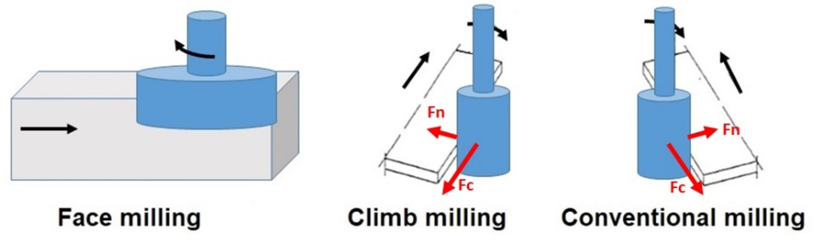
The first studies on machining of CMCs, and in particular of Cf/SiC (Sepcarb-Inox^®), were carried out in the 1990s by Danglot, J. [3] and Girot, F. [4], in collaboration with diamond tool manufacturers. Sepcarb-Inox^® (45 vol% of woven carbon fiber, 50 vol% CVI silicon carbide matrix, and 5 vol% of porosity) contour milling or trimming is the least known machining method. Planning or face-milling operations are quite limited (Figure 3).

Edging/trimming is the mandatory operation that can be carried out several times during the production cycle of the material to open the pores and continue the infiltration process, eliminate excess lengths, and obtain the final dimensions. It can be compared to a deep pass grinding operation since the radial passes can be several mm.

A priori, there is no difference between climb or conventional machining, since, in grinding, the advance of the table changes direction with each pass. This point has been confirmed by Danglot [3]. In conclusion, the works of Danglot and Girot demonstrated the following:

(1) The grinding wheel is a fundamental factor for machining. The quality of machining depends on its characteristics and its reproducibility. The choice of grains should be limited to ranges with little grain size disparity. Making the tool with electrolytic binder with a normal crimp (50%) should allow the useful life of the tool to be increased by at least 30% for an equivalent purchase cost. This new embedment height should improve the tool’s cutting ability, with clearer cutting edges and better chip evacuation. During the first machining operations with this type of tool, it will be necessary to check that the diamond grains are not expelled from the bond under the cutting force, which would reduce the useful life of the tool. If we limit the shear stress, this phenomenon should not occur.

(2) Analysis of the material before machining reveals multiple porosities and cracks in the matrix. Machining generates new cracks as well as chipping of the material throughout and at the end of machining. This can be detrimental to the mechanical characteristics of the material. Measurement of the specific longitudinal Young’s modulus before and after machining indicates a decrease in this characteristic when the cutting force exceeds 50 N. The surface finish does not change with increasing cutting depth. It improves noticeably if the rotation speed is high. The dimensions of the chipping on the surface of the material increase if the depth of cut is increased and if the rotation speed is decreased. No delamination was observed. This is explained by the fact that there are no forces in the interlaminar direction.

(3) Cutting forces change depending on parameters. They increase linearly with cutting depth and feed speed. They decrease exponentially depending on the rotation speed of the tool. The range of forces recorded is very wide, from 1 N to 320 N. The radial force is mainly related to the rotation speed. The other parameters—feed, depth of cut, and their interactions with rotation speed—have much less influence. Tangential force is a function of speed, depth of cut, and their interactions. These variables have the same weight in increasing the tangential force for consistent work. In the case of conventional milling, the tangential force is multiplied by 2 to 4. Climb milling should be used systematically to limit cutting forces.

(4) Machining in grinding conditions (very high rotation speed, very fast feed, and low cutting depth), as recommended by tool manufacturers to limit the cutting force, is not the right solution. Machining with the milling conditions (moderate rotation speed, limited feed, and high depth of cut) allows a high material removal rate with moderate cutting forces.

Recently, An et al. [5] provided a detailed literature survey on the machining of C-SiC. The material removal mechanism, defect form, and interfacial mechanical properties were summarized. Preliminary experiments have proved that ultrasonic-assisted machining has shown unique advantages in reducing force and tool wear, improving machining quality and machining efficiency.

Diaz et al. [6] provided an informative literature survey of the research undertaken in the field of conventional and non-conventional machining of CMCs with a main focus on critically evaluating how different machining techniques affect the machined surfaces.

Wang et al. [7] observed and analyzed the failure modes of the SiC matrix and carbon fiber under ordinary cutting and ultrasound cutting conditions. With the help of ultrasonic energy, the grinding force is reduced up to 60%, which means that ultrasonic vibration is beneficial to reduce the grinding force.

Luna et al. [8] evaluated the influence of grit geometry and fiber orientation on the abrasive material removal mechanisms of SiC/SiC ceramic matrix composites (CMCs). They demonstrated that the shape of the abrasive grits has a stronger influence on the measured process forces. As the size of grit is decreased, less resistance to penetration is encountered by the grit to engage the workpiece in matrix-rich areas. The scratch tests with arrangements of multiple grains demonstrated the ability of SiC/SiC CMCs to arrest the lateral cracks governing the material removal in brittle mode.

2.3. Abrasive Tools

The tools used for this type of machining are of two categories: concretion wheels, and abrasive wheels with electrolytic binder (Figure 4).

Concretion wheels are wheels whose diamonds are completely covered by the binder, sintering the active zone of the tool on the metal support. The binder can be metallic (bronze, etc.) or resinoid (bakelite). The advantages of these tools are their longevity (several layers of diamond) and the good condition of the machined surfaces. Their disadvantages are cost and low removal rate.

Electrolytic bond grinding wheels have only one or two layers of diamond. The diamond is attached to the metal frame of the tool, thanks to an electrolytic (nickel) deposit. This tool has a much lower unit cost and its known drawback is a random and shorter useful life than that of concretion wheels. However, it has an affordable price and an excellent cutting power.

The diamond is natural, with a maximum diamond concentration (volume of diamond deposited on the tool), meaning that the grains touch each other around the entire periphery. A so-called aerated concentration can be requested from the tool manufacturer to limit the so-called “jamming” or dulling problem of the tool, although it is not usually used to machine this type of material due to a limited number of diamond grains. The crimping corresponds to the embedding height of the diamond grains in the electrolytic deposit. There are three heights: (i) D or low (30% embedding), (ii) N or normal (50% embedding), and (iii) S or super (75% embedding) [9].

Usually, the tools used are those with S embedding, as they resist better during the machining of Cf/SiC and SiCf/SiC. Concerning grain size, grinders with grit D427 (roughing) to D151 (finishing) are used. The grain size influences the machined surface. A large grit allows an interesting material removal rate in a short time, but leaves very marked scratches on the piece that will have to be removed with a fine-grain grinding wheel. A D252 grain was chosen, which is a medium grain size with good cutting power, to machine with large cutting depths. Additionally, this grit size is often used for grinding wheels where the dimensional accuracy of the tool is not essential.

2.4. Wear of Abrasive Tools

Determining the wear of an abrasive tool in the machining of ceramic matrix composites (CMCs) is crucial for maintaining the quality of machined parts and optimizing tool life. The wear of abrasive tools in CMC machining can be assessed using various methods and observations:

➢

Visual inspection: Start with a visual inspection of the abrasive tool. Look for signs of wear on the tool’s surface, such as (i) loss of sharpness on abrasive grains or edges; (ii) formation of chips, cracks, or fractures on the abrasive material; or (iii) change in color or surface texture due to wear. Early signs of wear may not be immediately obvious, so regular inspections are important.

➢

Measurement of tool dimensions: Measure the key dimensions of the abrasive tool before and after machining CMCs. These dimensions can include diameter, thickness, mass, and any relevant geometrical features. A reduction in these dimensions can indicate wear.

➢

Tool wear rate calculation: Calculate the tool wear rate using the following formula:

$$Tool Wear Rate \left(Vw\right)=\frac{\left(Initial Tool Dimension-Final Tool Dimension\right)}{Total material removed}$$

This calculation provides a quantitative measure of how much material the tool has lost due to wear.

➢

Surface finish analysis: Evaluate the surface finish of the machined CMC parts. As the tool wears, it may produce surface defects such as chattering, scratches, or poor finish quality. A noticeable deterioration in surface finish can be an indicator of tool wear.

➢

Cutting forces monitoring: Monitor the cutting forces during machining. A sudden increase in cutting forces or abnormal fluctuations can suggest tool wear. You can use force sensors or dynamometers to accurately measure cutting forces.

➢

Acoustic emission analysis: Acoustic emission monitoring can detect subtle changes in tool wear by analyzing the sound emitted during machining. Abrupt changes or unusual patterns in acoustic emission signals can indicate tool wear [10].

Regularly assessing and managing abrasive tool wear is essential to maintain machining efficiency, product quality, and tool life when working with ceramic matrix composites. The machining parameters, tool selection, and maintenance practices should be adjusted based on the wear analysis findings to optimize the process.

Apart from dimensional or mass measurements, there is therefore no quantification of the wear of the abrasive tool. Furthermore, this dimensional or mass measurement does not provide additional information on the wear process of the abrasive tool (grain wear or cleavage) nor on the abrasive power of the tool at a given time for the machining operation.

3. Fractals for Wear Modeling and Control

3.1. The Importance of Wear of Diamond Tools for Machining CMCs

Tool wear prediction is one of the most important topics in the field of machining. The prediction of tool wear is mainly related to the integrity of the surfaces, and it directly affects the quality of the part and is important at the level of production logistics and manufacturing costs [11].

There is some information on the wear of diamond-coated tools for applications other than machining with CMCs, for example, methodologies for measuring tool wear in rock machining [12], or mathematical models for calculating the Blunting Area, taking into account different wear mechanisms [13]. There is abundant information on predicting the wear of conventional tools when machining metals, and with very diverse approaches: (i) the use of analytical models and neural networks in turning [14], (ii) signal analysis with treatment using neural networks for milling [15], (iii) use of linear regressions in combination with design of experiments in finishing operations [16], or (iv) use of algorithms in combination with “Machine Learning” [17].

3.2. The Use of Fractals for Machining Analysis

Topology, as a geometry, is extended to the definition of fractal structures by characterizing equivalences in different levels of detail. In the investigation of Sahoo et al. [18], an exhaustive examination is conducted of the use of fractals to characterize the surface quality of various machining processes. It is mentioned that one of the main advantages of this approach is the independence of the sample size. For example, height variations in roughness depend on the size of the section being analyzed. Using a measure that is scale invariant [19] suggests the use of fractals in the case of surfaces that are rough (such as those of diamond abrasive tools).

For this research, a plate of silicon carbide CMCs was machined by edging. The useful height of the abrasive tool was 10 mm, and the thickness of the composite plate was 6.5 mm. The tool was centered symmetrically with respect to the composite plate, such that approximately 1.75 mm on each side of the tool remained unused, which served as a sample to determine the difference in the fractal dimension of the tool in “new” condition.

A convenient way of characterizing the roughness of a surface (or to characterize a diamond abrasive-type tool) is Hausdorff or fractal dimension. A fractal geometry is a measure of the complexity of the surface, and the value of the fractal dimension can take a non-integer value between 2 and 3. In general, when the value of the fractal dimension increased, the greater the complexity of the surface. For smooth surfaces, the value of fractal dimension is near to 2, which gradually increases with an increment in roughness of the surface. For drastically rough surfaces, the fractal dimension comes close to 3.

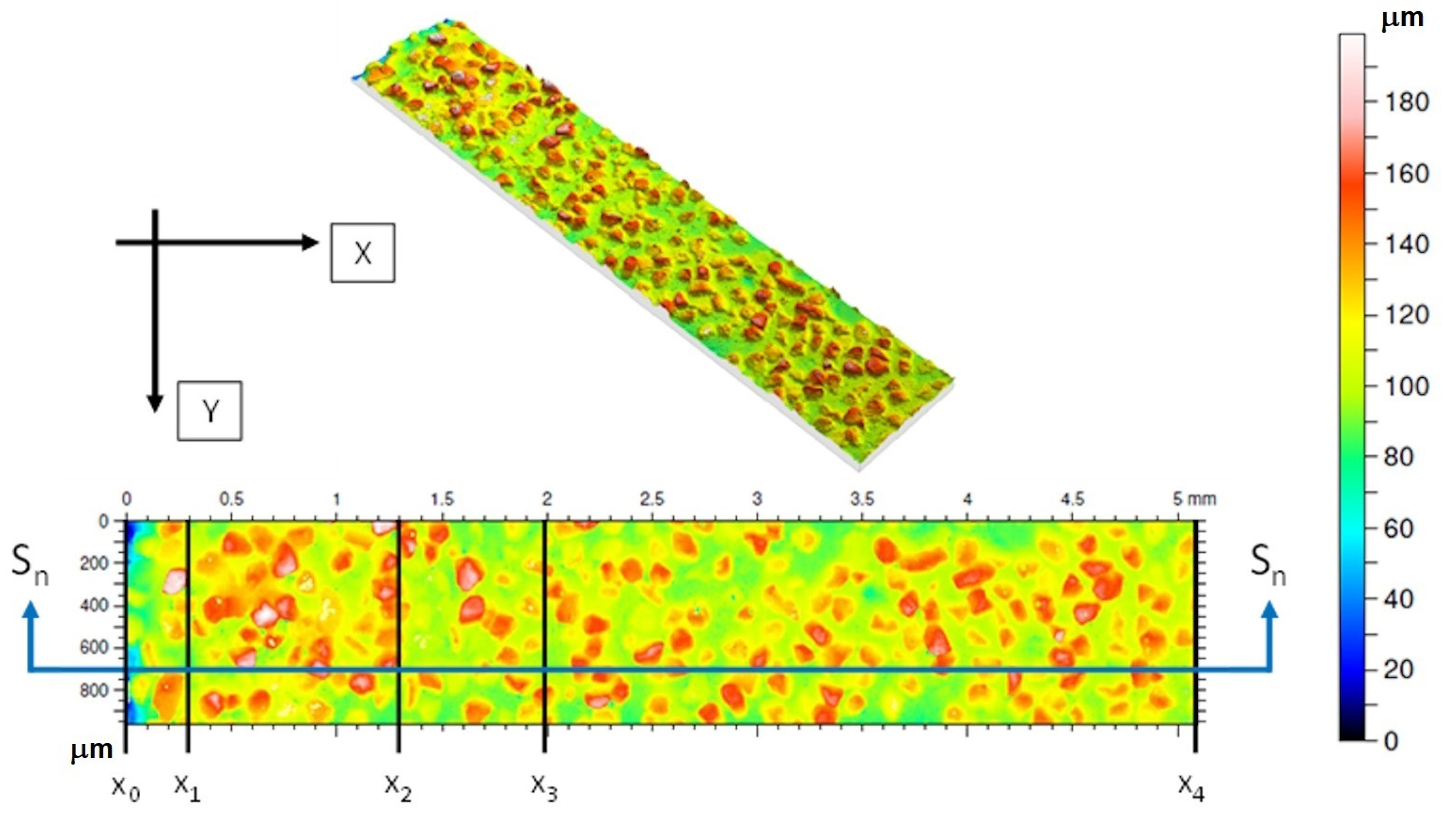
There is a variety of proposals to calculate the fractal dimension of a surface: using triangular prisms [20], the variation method [19,21], box counting [22], the three-dimensional root mean square (3D-RMS) [23], the regional residual root mean square (3R method) [24], the cubic covering method, or the surface area method [25,26]. All of the above methods have advantages and disadvantages and greater or lesser precision. However, they all have a limitation regarding the shape of the area that is sampled to determine the fractal dimension (the measured section must be square), or the number of sample points on the map at each coordinate of the XY plane (it must be a number close to a power of 2). An example of a “problematic” data map is shown in Figure 5.

For a topographic map such as the one in Figure 5, it is difficult to calculate the fractal dimension, since the entire section of the tool has not been worn. The tool edge will not be taken into account, from the dimension x₀ = 0 to x₁ = 0.3 mm. The data between the coordinates x₁ = 0.3 to x₂ = 1.3 mm correspond to the area where the abrasive tool has not machined CMC. The area from x₃ = 2 to x₄ = 5.1 mm is where machining has occurred. Between x₂ = 1.3 and x₃ = 2 mm there is uncertainty regarding the location of the tool with respect to the CMC plate during machining, and that is why it was not analyzed.

3.3. Proposed Method to Determine the Fractal Dimension

The surface must meet certain minimum requirements to be able to be analyzed according to the method that will be proposed later. The requirements are:

-

The roughness must be isotropic: the surface must not present directionality in its fractal pattern. The isotropy of the surface is important since it allows the dimension reduction method to be used to calculate the surface fractal (D_surf) as the fractal dimension value along a certain direction of a profile (D_prof) + 1 [20,24]. An example of isotropic and anisotropic roughness is shown in Figure 6.

-

The section (map) from which the fractal dimension will be calculated must be square or rectangular in shape, and must be aligned along a convenient coordinate system, as shown in Figure 2.

The proposed method consists of the following steps:

-

Divide the surface into sections along the direction containing the greatest quantity of data, and obtain roughness profiles perpendicular to the direction containing the least quantity of data. In the case of Figure 5, the largest quantity of data is along the X coordinate (columns) and the direction with the least quantity of data is along the Y direction (rows).

-

The selection of the roughness profile will depend on the area of the surface to be analyzed. For example, Figure 7 shows a roughness profile from x₃ = 2 to x₄ = 5.1 mm, in the area where the tool has machined CMC.

-

The number of roughness profiles will be equal to the smallest number of data along that direction; in the case of Figure 5, from n_row = 1 (y = 0 mm) to n_row = 96 (y = 0.95 mm).

-

Calculate the fractal dimension for the section of each roughness profile as shown in Figure 5. To calculate the fractal dimension, the power spectral density (PSD) method is recommended [27]. Each coordinate on the X axis represents time in a wave, and the amplitude of the same wave is represented by the roughness height on the Z coordinate.

-

Power spectral density requires the selection of a way to estimate the energy of the wave (in this case the roughness profile). One can use the classic methods: “method of autocorrelation method, periodogram method, Bartlett method, and Welch method”. According to Shen et al. [28], the Bartlett and Welch methods are the most precise, and that is why the latter (Welch) has been selected.

-

For each profile, the slope (β) is calculated on a log–log scale of the fit line for the power spectral density data [29], as shown in Figure 8 for the roughness profile in Figure 7.

-

The slopes are calculated for all surface roughness profiles in the study area of interest from n_row = 1 to n_row (as in the case of Figure 5), and the value of the Hurst coefficient (H) is calculated, with 0 ≤ H ≤ 1 [27], from Equation (1).

$$\left|\beta \right|=2H_{n_{row}}-1$$

(1)

For a self-affine surface [19], the fractal dimension of the surface (2D) from its roughness profiles (1D) will be calculated using Equation (2).

$$D_{{surf n}_{row}}=E+1-H_{n_{row}}$$

(2)

where E is the dimension of the Euclidean space (in this case E = 2 for a surface).

-

The estimated values $D_{{surf n}_{row}}$ of each roughness profile are adjusted to a logistic type distribution [30]. The logistic distribution was chosen due to its relative simplicity and because it adapts very well to the way in which the $D_{{surf n}_{row}}$ data obtained from each roughness profile are distributed (Figure 9).

-

The value of $D_{surf}$ for the entire fractal surface is given by Equation (3).

$$D_{surf}=\mu \left[PDF\left(D_{{surf n}_{row}}\right)\right]$$

(3)

where µ is the value of the location parameter of the probability density function (PDF).

4. CMC Abrasive Machining Experiments

4.1. Material Used in the Abrasive Machining Tests

The material was supplied by SGL CARBON GmbH (Wiesbaden, Germany). This company offers both Cf/C (SIGRABOND^® Standard) and Cf/SiC (SIGRASIC^®) CMCs. This last material can be adapted to the required application with a behavior controlled by the matrix (matrix dominated with milled fibers (MFs)), mixed (short fibers (SFs)), or controlled by the reinforcement (fiber-dominated with long fibers (LFs)). SIGRASIC^® LF was selected because it is the type of material used in aircraft engine applications [31].

Cf/SiC is manufactured by infiltrating a carbon fiber-reinforced carbon body with silicon (Figure 10). Due to near net shape processing, complex machining can be performed cost-effectively early in the process. Final ceramic grinding can be used locally when tight tolerances are required. By suitable adjustment of the material and process parameters, the product characteristics can be matched to the intended use of the CMC component (Figure 10). The mechanical properties are shown in Figure 11. The test pieces are 100 × 100 × 6.5 mm³ plates.

4.2. Tools and Machining Equipment

The diamond wheels were supplied by the PFERD company [9], and had the characteristics defined in

Table 1. Characteristics of the abrasive grinder used in the study.

Abrasive Tool Reference	Type	Vc	Feed	Pass
DZY-N 25.0 10/12 D126	Diamond 106–125 μm	15–25 m/s wet	0.01–0.05 mm/rev	≤6 mm

.

The machining center used for the tests was a KONDIA A6 vertical axis, mobile table machine, with a spindle rotation capacity of 15,000 rpm. External lubrication based on coolant was used.

For these preliminary tests, a 25 mm diameter tool with diamond grains was used because it offers a range of wet cutting speed compatible with the limitations of the equipment (15,000 rpm, but limited to 13,000 rpm).

In order to compare the results with other research works, the cutting speed was 2, 7, 12, and 17 m/s. The feed speed was 100, 500, and 1000 mm/min (

Table 2. Design of experiments performed.

Ref.	Vc (m/s)	N (rpm)	Feed Vf (mm/min)	Pass ae (mm)
[1]	2	1529	100	1
[2]	7	5350	100	1
[3]	12	9172	100	1
[4]	17	12.994	100	1
[5]	17	12.994	500	1
[6]	12	9172	500	1
[7]	7	5350	500	1
[8]	2	1529	500	1
[9]	17	12.994	1000	1
[10]	12	9172	1000	1
[11]	17	12.994	100	2.5
[12]	7	5350	1000	1

).

The tests were performed using a constant axial pass, corresponding to the thickness of the composite plate (6.5 mm), and a fixed radial pass of 1 mm, except for a test where it was increased to 2.5 mm in order to conduct a deep pass test and see its influence on the cutting forces.

A Kistler dynamometer was used to analyze the forces in the three orthogonal directions (Figure 12). The device follows ISO 376 [32] and ASTM E74 [33] standards for calibration and verification for force measuring, and is calibrated every 6 months.

The material was climb machined according to the results of Danglot’s study [3].

4.3. Damage Measurement Methodology

To determine the quality of the cut and its impact on the damage to the CMC material, two variables representative of the process for different cutting conditions were measured from pictures and using the image analysis software ImageJ [34]. ImageJ is public domain digital image processing software programmed in Java, developed at the National Institutes of Health. Those variables were the maximum depth of chipping (in μm) and the linear chipped area (in mm²/cm). To do this, the color picture was changed to a black and white one and digitized (Figure 13).

The magnification of the image is defined from a known measurement or an initial calibration and all black particles in the digitized photo are determined.

For each cutting condition, different pictures are taken along the 100 mm machined. These surfaces are averaged and a specific damage is determined for the measured surface corresponding to 10 mm in length (linear chipped area). The maximum width of the chipping along the 100 mm (maximum chipping) is also determined.

5. Wear Results

5.1. Tool Wear Evolution

The evolution of tool wear was carried out by determining the fractal dimension of the tool surface of a worn area and comparing it with the fractal dimension of the part of the tool that was not machined by the CMC.

The values obtained following the methodology described above are reflected in

Table 3. Values of the fractal dimension of the tool surface as a function of the test number and the cutting force applied to the tool.

Test Number	D_surf	R2	Fc (N)	ΔD_surf
0	2.1896	0.9889	0	0
1	2.1902	0.9524	20.65	0.0006
2	2.1132	0.9532	12.35	−0.077
3	2.0982	0.9488	13.77	−0.015
4	2.1731	0.8761	11.06	0.0749
5	2.0594	0.9649	27.92	−0.1137
6	2.1228	0.9534	28.56	0.0634
7	2.1403	0.9043	40.53	0.0175
8	2.0427	0.9743	52.15	−0.0976
9	2.1068	0.9634	25.23	0.0641
10	2.1916	0.8921	27.17	0.0848
11	2.0815	0.9627	20.54	−0.1101
12	2.1336	0.9278	55.86	0.0521

. The variation in the fractal dimension with respect to the previous test was also calculated; this variable that can explain how wear occurs and develops.

The corresponding images obtained with the Leica DCM 3D confocal microscope are given in Appendix A (top view and 3D view of the tool surface analyzed) and in Appendix B (optical view of corresponding zone), after each of the different tests 1 to 12.

As we are dealing with a 3D surface, the fractal dimension has a value between 2 and 3. If the wear is homogeneous, meaning the grains are worn away and lead to a flat surface, the fractal dimension should decrease and approach the value 2.

If, on the other hand, wear is produced by breaking the grains, or if other smaller grains appear on the surface, the surface of the tool will be rougher and its fractal dimension will increase to move away from the value 2.

Figure 14 details the evolution of the fractal dimension with the cutting force applied to the tool. A decreasing evolution of the fractal dimension with cutting force is highlighted, meaning that, for the higher the cutting load, the smaller the fractal dimension, resulting in greater wear.

However, the trend is that there is no clear relationship between the fractal dimension and the cutting force.

However, interesting things may appear when analyzing the variation of the fractal dimension with respect to the previous test (Figure 15). In this figure, one can notice positive or negative variations. Negative variations are associated with a decrease in the fractal dimension, which corresponds to a smoother surface or a regular wear of the grains. Positive variations are associated with the cleavage of diamond grains and the appearance of new underlying grains. These variations also depend on the level of the cutting or feed force acting on the tool, which have a particular influence on the diamond grain behavior.

The height of the diamond grains decreases with wear but is also dependent on the force applied to the abrasive tool. The higher the cutting load, the greater the wear or breakage of the grains (Figure 16). It has been proven that, during the wear of the grains, several of them cracked due to an inappropriate grain crystallographic orientation with respect to the cutting forces. These cracks lead to partial rupture of the grain by cleavage (which occurs in test 4) or due to excess of cutting force. Figure 17 highlights these different aspects. The new abrasive tool has some grains with cleavage (bright points in Figure 17a). When wear evolves, the quantity of grains presenting a smooth face increases (end of test 3, Figure 17b). If machining continues, grain cleavage is greater compared to worn grains (end of tests 4 and 12, Figure 17c,d).

Another interesting evolution concerns the diamond abrasive height as a function of the tool surface fractal dimension (Figure 18). This height decreases continuously from test 1 to test 12. Sequences of grain wear are followed by steps of grain cleavage or breaking, hence decreasing and increasing the fractal dimension of the tool surface. Smaller grains also surface in the cutting zone and participate in the abrasion machining of the CMC, contributing to an increase in the fractal dimension.

5.2. Multiple Linear Regression of Fractal Dimension

The analysis of variance (

Table 4. Analysis of variance of the fractal dimension D_surf.

Variable	Coefficient	Standard Deviation	t Student	Confidence %	Risk %
Fc	0.1055	0.0298	3.5441	99.47	0.53
ae	2.1531	0.4638	4.6423	99.91	0.09
Fc. ae	−0.1065	0.037	−2.8775	98.35	1.65
Source	Square sum	DoF	Mean squares	Fisher	Confidence %	Risk %
Regression	53.9936	3	17.9979	37.3736	100	0
Residues	4.8157	10	0.4816
Total	58.8093	13	4.5238		R = 0.9582

) was realized with LUMIERE 5.40 software and demonstrates that the fractal dimension of the surface can be explained by the variations in significant parameters such as the cutting load Fc, the radial pass ae, and the interaction of these two parameters. The regression coefficient of the model is also quite good (R = 0.9582).

On the other hand, it was not possible to define a model that explains the evolutions of the fractal dimension variation ΔD with respect to the previous test.

6. Relationships between Wear, Forces, Damage, and Roughness

The results of evolution of the machining loads, damage and roughness are given in

Table 5. Evolution of the machining loads, CMC damage, and roughness during the different tests performed. Sa (arithmetical mean height), Sz (maximum height), and Sq (root mean square height) are the surface texture parameters of the machined sample.

Test Number	Chipped Area mm2/cm	Maximum Chipping μm	Fc N	Fn N	Sq μm	Sz μm	Sa μm
1	0.1729	105	20.65	2.72	23.8	309	18.5
2	0.0809	63	12.35	3.76	40.2	223	33.3
3	0.0589	57	13.77	4.51	26.3	162	20.9
4	0.0189	48	11.06	4.66	21.4	170	16.6
5	0.0591	55	27.92	1.81	30.7	208	24.5
6	0.1296	61	28.56	1.5	21.4	187	16.7
7	0.2329	113	40.53	2.11	27.5	189	22.1
8	0.2838	193	52.15	2.34	18	153	14.1
9	0.1665	106	25.23	1.47	28.4	217	22.7
10	0.2109	158	27.17	1.48	30.9	241	24.9
11	0.0383	117	20.54	1.67	44	352	36.3
12	0.4097	302	55.86	2.46	35.7	225	28.6

.

6.1. Evolution of Cutting Forces

The cutting load decreases with the cutting speed regardless of the feed velocity (Figure 19). This result is in agreement with the conclusion of Danglot’s work [3]. From 15 m/s, the cutting force practically no longer changes, justifying that it is not necessary to work at higher speed to reduce the forces on the tool. This is interesting since it means that a conventional machining center working at 15,000 or 25,000 rpm can carry out this type of machining using a tool with a diameter of 20 or 10 mm.

The normal force Fn is in all cases very small (<5 N) and in the uncertainty of the measurement (±5 N).

The difference in results with Danglot’s work, i.e., the efforts obtained are double, can be attributed to the materials used in one case (SEPCARB-INOX) or in the other (SIGRASIC^®).

Concerning the evolution of the cutting force with the feed speed (Figure 20), it appears that the force increases continuously with the feed speed for low cutting speeds (2 and 7 m/s). For higher speeds (12 and 17 m/s), the forces are very similar with a non-monotonic behavior and reach their maximum around 700 mm/min (30 N). This demonstrates that it is possible to have high productivity while maintaining low cutting force.

6.2. Multiple Linear Regression of Cutting Forces

The analysis of variance (

Table 6. Analysis of variance of the cutting force.

Variable	Coefficient	Standard Deviation	t Student	Confidence %	Risk %
ae	10.2834	2.3217	4.4292	99.87	0.13
Vf	0.0748	0.01	7.4545	100	0
Vf × Vc	−0.0037	0.0008	−4.844	99.93	0.07
Source	Square sum	DoF	Mean squares	Fisher	Confidence %	Risk %
Regression	11,299.5072	3	3766.5024	73.6568	100	0
Residues	511.3586	10	51.1359
Total	11,810.8658	13	908.5281		R = 0.9781

) demonstrates that the variations in the cutting force can be explained by the variations in significant parameters such as the feed velocity Vf, the radial pass ae, and the interaction between the feed velocity Vf and the cutting speed Vc. The regression coefficient of the model is also quite good (r = 0.9781).

6.3. Evolution of the Damage to the Material

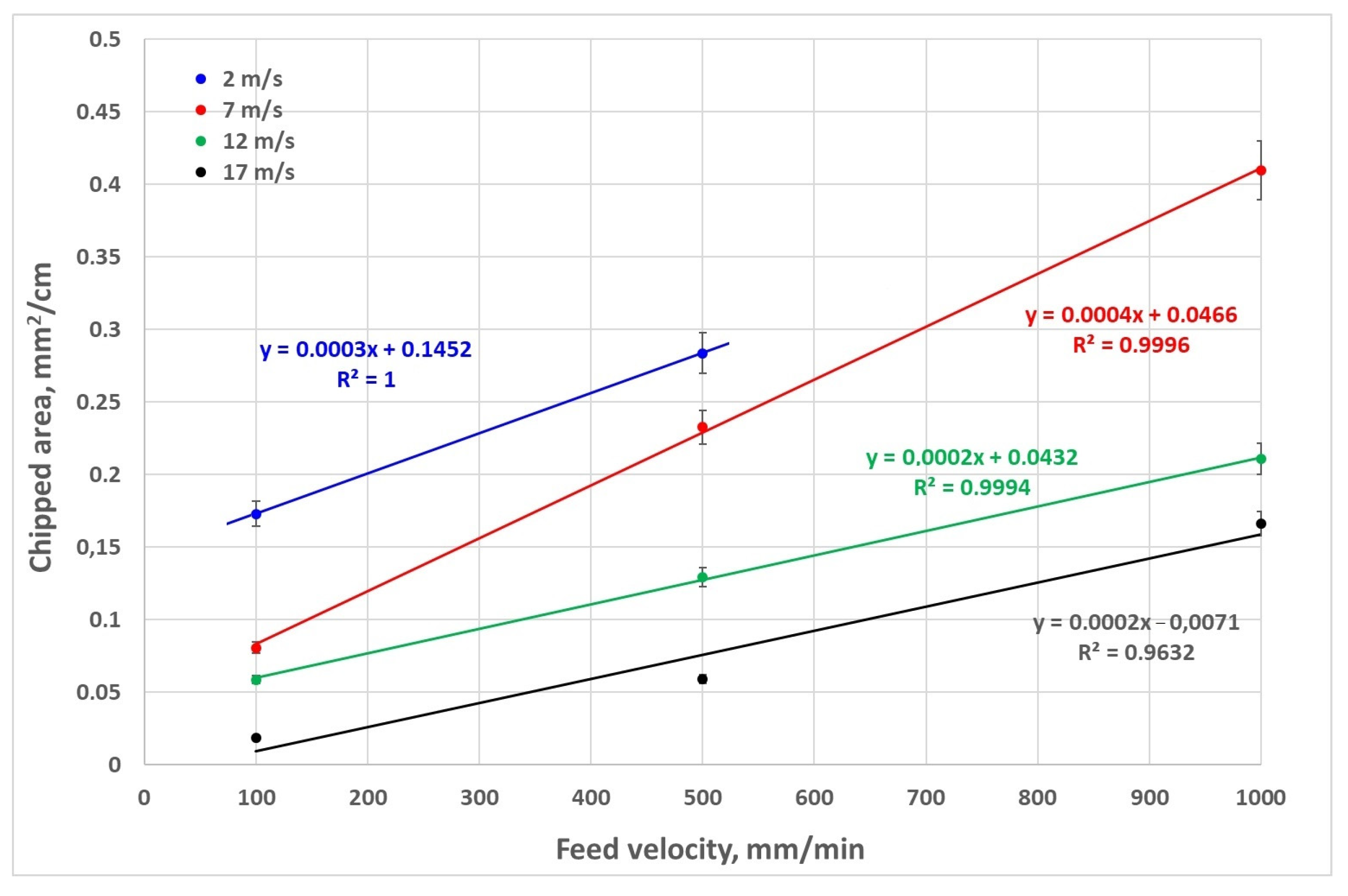
Concerning the evolution of the chipped area with the cutting speed, the higher the cutting speed, the lower the chipped area (Figure 21). Furthermore, in the case of the feed velocity, the higher the feed velocity, the higher the chipped area (Figure 22).

However, it should be noted that for cutting speeds of 12 and 17 m/s, this dependence of the chipped area on the feed speed is less significant than for cutting speeds of 2 and 7 m/s. The chipped area is therefore very dependent on the cutting speed.

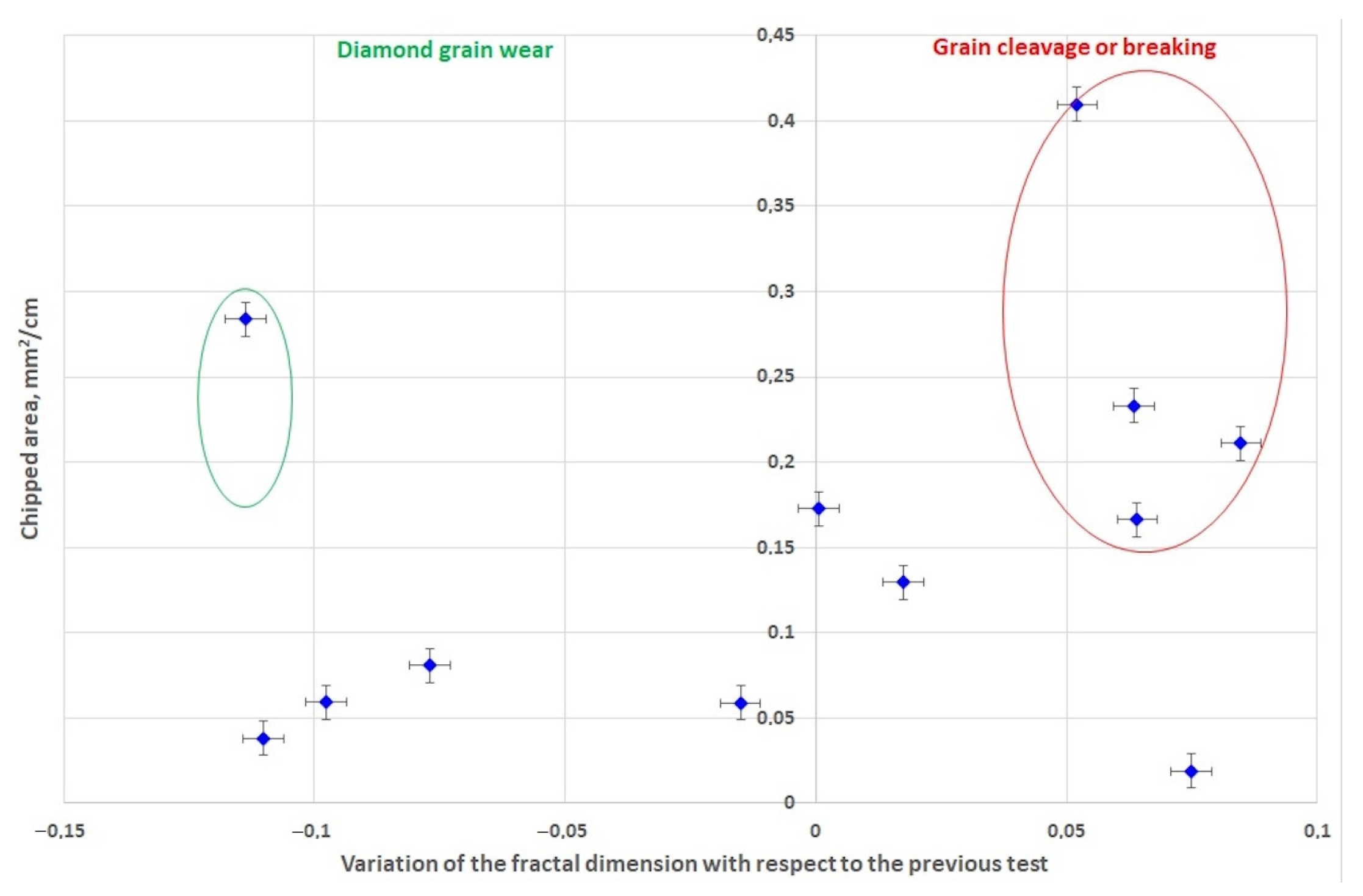
An interesting analysis concerns the evolution of the chipped area with the variation in the fractal dimension with respect to the previous test (Figure 23). This analysis highlights that the greater this variation (positive or negative), the greater the chipped area. However, this damage occurs more frequently when this variation is positive (associated with grain cleavage or rupture) than when it is negative (associated with diamond grain wear). So, this means that the damage mode of the tool has a strong influence on the chipped area of the CMC part.

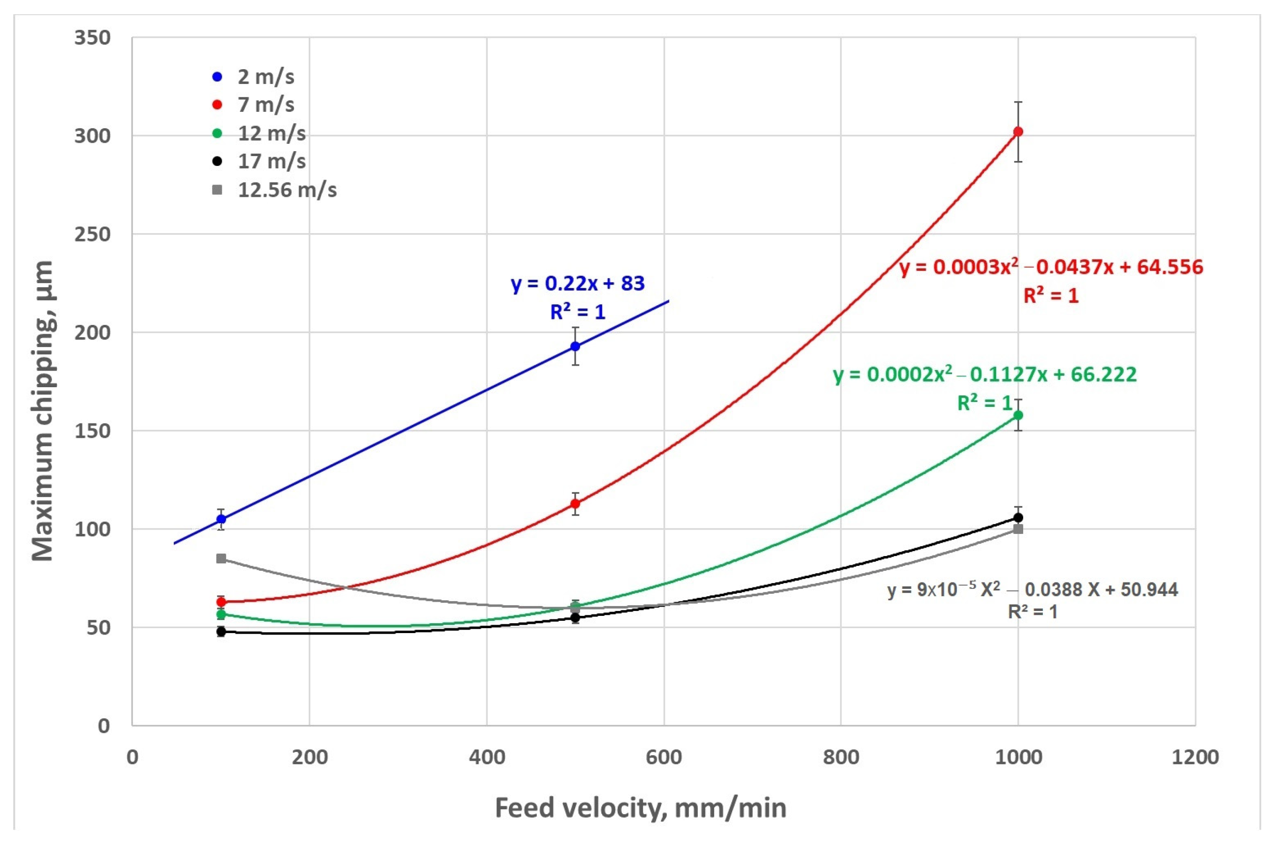
Concerning the maximum chipping, the evolution is similar. The higher the cutting speed or the lower the feed velocity, the lower the maximum chipping (Figure 24 and Figure 25). In this case, it should also be noted that for cutting speeds of 12 and 17 m/s, this dependence of the maximum chipping on the feed speed is less significant than for cutting speeds of 2 and 7 m/s.

Concerning the evolution of the maximum chipping with the variation in the fractal dimension with respect to the previous test (Figure 26), it is highlighted that the greater this variation (positive or negative), the higher the maximum chipping. However, unlike for the chipped area, the maximum chipping strongly depends on the variation in the fractal dimension compared to the previous test. For high variation values (worn diamond grain or cleavage), the maximum chipping is high. For variations in the fractal dimension less than −0.1 or greater than +0.05, the maximum pullout increases significantly, and is not conditioned by the type of damage to the tool.

6.4. Multiple Linear Regression of Chipped Area

The analysis of variance (

Table 7. Analysis of variance of the chipped area.

Variable	Coefficient	Standard Deviation	t Student	Confidence %	Risk %
Vc	−0.0092	0.0021	−4.3775	99.76	0.24
D_surf	0.0644	0.0127	5.0636	99.90	0.10
Vf × Vc	0.0000	0.0000	−3.1989	98.74	1.26
Vf × ae	0.0004	0.0001	7.1231	99.99	0.01
Source	Square sum	DoF	Mean squares	Fisher	Confidence %	Risk %
Regression	0.4305	4	0.1076	136.2415	100	0
Residues	0.0063	8	0.0008
Total	0.4369	12	0.0364		R = 0.9926

) demonstrates that the variations in the chipped area can be explained by the variations in significant parameters such as the cutting speed Vc, the fractal dimension D_surf, the interaction between the feed velocity Vf and the cutting speed Vc, and the interaction between the radial pass ae and the feed velocity Vf. The regression coefficient of the model is also very good (r = 0.9926). The interaction between the radial pass ae and the feed velocity Vf is representative of the metal removal rate (MRR) since, in our case, the axial depth ap is constant. The model points out that the higher the MRR, the higher the chipped area.

6.5. Multiple Linear Regression of Maximum Chipping

The analysis of variance (

Table 8. Analysis of variance of the maximum chipping.

Variable	Coefficient	Standard Deviation	t Student	Confidence %	Risk %
D_surface	19.0108	6.6851	2.8438	98.07	1.93
Vf × Vc	−0.0184	0.0031	−5.9483	99.98	0.02
Vf × ae	0.3552	0.0450	7.8854	100.00	0.00
Source	Square sum	DoF	Mean squares	Fisher	Confidence %	Risk %
Regression	210,992.6347	3	70,330.8782	85.4064	100.00	0.00
Residues	7411.3653	9	823.4850
Total	218,404.0000	12	18,200.3333		R = 0.9829

) demonstrates that the variations in the chipped area can be explained by the variations in significant parameters such as the fractal dimension D_surf, the interaction between the feed velocity Vf and the cutting speed Vc, and the interaction between the radial pass ae and the feed velocity Vf (interaction proportional to the MRR). The regression coefficient of the model is also very good (r = 0.9926).

6.6. Evolution of the Roughness of the CMC Sample

The surface texture parameters of the machined sample Sa (arithmetical mean height), Sz (maximum height), and Sq (root mean square height) in ISO25178 were measured using a Leica DCM 3D system with dual core technology that combines confocal and interferometry technology for high-speed and high-resolution measurements down to 0.1 nm.

There is no notable pattern that relates the roughness Sq, Sz, or Sa to the process parameters, cutting speed, or feed rate.

At a feed speed of 1000 mm/min, the roughness parameters appear constant.

The roughness values Sq and Sa evolve in a similar way. Up to a cutting speed of 14 m/s, the parameters Sq and Sa seem to decrease when the feed speed increases. Above that value, the result is the opposite.

The roughness Sz decreases with the cutting speed at low feed rates, but increases with a feed rate of 500 mm/min.

There is also no clear pattern of evolution of roughness with advance speed.

At 100 mm/min and 1000 mm/min, the best results are associated with a cutting speed of 17 m/s.

At 500 mm/min, roughness is minimized with a low cutting speed (2 m/s).

Since SIGRASIC-LF is a material manufactured by liquid and gas infiltration, there could be a relationship between the microstructure of the material, and especially the closed and reopened porosities during machining, and the results of roughness measurements. Figure 27 presents micrographs of the machined surface in the central part of the material where the porosities reopened during machining can be seen. There are no differences in porosity between the different cutting conditions that could explain the roughness results and that could be attributed to the quality and microstructure of the material.

6.7. Multiple Linear Regression of Roughness Sa

The analysis of variance (

Table 9. Analysis of variance of the roughness Sa.

Variable	Coefficient	Standard Deviation	t Student	Confidence %	Risk %
ae	9.6457	3.8650	2.4956	96.83	3.17
D_surf	5.8533	2.1842	2.6799	97.69	2.31
Source	Square sum	DoF	Mean squares	Fisher	Confidence %	Risk %
Regression	6682.2530	2	3341.1265	104.8799	100.00	0.00
Residues	318.5670	10	31.8567
Total	7000.8200	12	583.4017		R = 0.9770

) demonstrates that the variations in the roughness Sa can be explained by the variations in significant parameters such as the fractal dimension D_surf and the radial pass ae.

6.8. Multiple Linear Regression of Roughness Sz

The analysis of variance (

Table 10. Analysis of variance of the roughness Sz.

Variable	Coefficient	Standard Deviation	t Student	Confidence %	Risk %
ae	94.9904	29.0894	3.2655	99.15	0.85
D_surf	53.3817	16.4389	3.2473	99.12	0.88
Source	Square sum	DoF	Mean squares	Fisher	Confidence %	Risk %
Regression	599,370.4741	2	299,685.2370	166.0718	100.00	0.00
Residues	18,045.5259	10	1804.5526
Total	617,416.0000	12	51,451.3333		R = 0.9853

) demonstrates that the variations in the roughness Sz can be explained by the variations in significant parameters such as the fractal dimension D_surf and the radial pass ae.

6.9. Multiple Linear Regression of Roughness Sq

The analysis of variance (

Table 11. Analysis of variance of the roughness Sq.

Variable	Coefficient	Standard Deviation	t Student	Confidence %	Risk %
ae	11.1078	4.4838	2.4773	96.73	3.27
D_surf	7.7930	2.5339	3.0755	98.83	1.17
Source	Square sum	DoF	Mean squares	Fisher	Confidence %	Risk %
Regression	10,355.9493	2	5177.9746	120.7717	100.00	0.00
Residues	428.7407	10	42.8741
Total	10,784.6900	12	898.7242		R = 0.9799

) demonstrates that the variations in the roughness Sq can be explained by the variations in significant parameters such as the fractal dimension D_surf and the radial pass ae.

For all these regression analyses, the normality test of the residuals demonstrates that the distribution is normal. This means that the models defined for each of the responses studied (fractal dimension D_surf, cutting force, chipped area, maximum chipping, and roughness values Sq, Sz, or Sa) do not require the addition of other parameters. The variations in the parameters of each of the models are sufficient to explain the variations in each of the responses.

7. Conclusions

This contribution demonstrated that the use of fractal dimensions to evaluate the wear of abrasive tools is an interesting method that allows more information to be obtained about the behavior of the grinding wheel than a simple dimensional or mass measurement.

The cutting forces and the fractal dimension of the tool surface are directly linked, and changes in cutting conditions can be highlighted by variations in this fractal dimension. Likewise, the type of damage to the abrasive tool (wear of the diamond grains, cleavage, or breakage, etc.) has a direct impact on the values of the fractal dimension.

The proposed method is therefore interesting but requires (i) having a confocal microscope available, (ii) dismantling and indexing the abrasive tool to systematically analyze the same zone(s), and (iii) gathering results from additional measurement time and investment in measurement equipment. On the other hand, the method ensures a certain quality of machining and control of material damage while ensuring better productivity.

The study also showed that milling cutting conditions make it possible to machine CMC with good productivity, while minimizing cutting forces and damage to the CMC (chipped area, maximum chipping). A cutting speed from 15 m/s combined with a feed speed of 500 mm/min allows this material to be optimally machined for cutting depths ae of up to 2.5 mm.

In the models developed to predict damage to the CMC (chipped area, maximum chipping) or the roughness of machined surfaces, the fractal dimension appears systematically as a significant parameter.

The fractal dimension D_surf is directly proportional to the cutting force Fc and to the radial depth of cut, which a priori is logical since the damage to the diamond grains depends on the engagement of the tool (hence ae) and of the force Fc applied during machining.

The chipped area depends mainly on the product Vf*ae and the fractal dimension D_surf, characteristics of the metal removal rate, the state of damage of the abrasive tool, and then, to a lesser extent, the cutting speed.

The maximum pull-off also mainly depends on the product Vf*ae and the fractal dimension D_surf.

The roughness values Sa, Sz, and Sq depend on the radial pass ae and the fractal dimension D_surf, characteristics of the engagement of the tool in the CMC material, and the state of damage of the abrasive tool.

In conclusion, the fractal dimension D_surf is therefore a good indicator of the wear of the abrasive tool and makes it possible to characterize both the damage of the tool and that of the machined material. The method proposed for determining this fractal dimension seems suitable for this type of application (abrasive machining).

References

- Klocke, F.; Klink, A.; Veselovac, D.; Aspinwall, D.K.; Soo, S.L.; Schmidt, M.; Schilp, J.; Levy, G.; Kruth, J.-P. Turbomachinery component manufacture by application of electrochemical, electro-physical and photonic processes. CIRP Ann. 2014, 63, 703–726. [Google Scholar] [CrossRef]
- Available online: https://www.marketsandmarkets.com/Market-Reports/ceramic-matrix-composites-market-60146548.html; (accessed on 24 October 2023).
- Danglot, J. Usinage des Matériaux Composites Thermostructuraux à Matrice Céramique, Mémoire CNAM nº258. Industrial Mechanics Engineer, CNAM, Paris, France, 17 June 1993. Available online: https://www.cetim.fr/formation/formation/production/Procedes-de-production/decolletage-usinage/usinage-des-materiaux-composites-a-matrice-organique-s17 (accessed on 5 November 2023).
- Girot, F.; Lartigau, J.P.; Cat, P. High-speed abrasive milling of ceramic matrix composite materials. In Proceedings of the 1st French and German Conference on High Speed Machining, Metz, France, 24–27 June 1997; pp. 351–355. [Google Scholar]
- An, Q.; Chen, J.; Ming, W.; Chen, M. Machining of SiC ceramic matrix composites: A review. Chin. J. Aeronaut. 2021, 34, 540–567. [Google Scholar] [CrossRef]
- Diaz, O.G.; Luna, G.G.; Liao, Z.; Axinte, D. The new challenges of machining Ceramic Matrix Composites (CMCs): Review of surface integrity. Int. J. Mach. Tools Manuf. 2019, 139, 24–36. [Google Scholar] [CrossRef]
- Wang, D.; Lu, S.; Xu, D.; Zhang, Y. Research on Material Removal Mechanism of C/SiC Composites in Ultrasound Vibration-Assisted Grinding. Materials 2020, 13, 1918. [Google Scholar] [CrossRef]
- Luna, G.G.; Axinte, D.; Novovic, D. Influence of grit geometry and fibre orientation on the abrasive material removal mechanisms of SiC/SiC Ceramic Matrix Composites (CMCs). Int. J. Mach. Tools Manuf. 2020, 157, 103580. [Google Scholar] [CrossRef]
- Available online: https://es.pferd.com/en/service/downloads/ (accessed on 9 September 2023).
- Liu, C.-S.; Ou, Y.-J. Grinding Wheel Loading Evaluation by Using Acoustic Emission Signals and Digital Image Processing. Sensors 2020, 20, 4092. [Google Scholar] [CrossRef]
- Attanasio, A.; Ceretti, E.; Giardini, C. Analytical Models for Tool Wear Prediction During AISI 1045 Turning Operations. Procedia CIRP 2013, 8, 218–223. [Google Scholar] [CrossRef]
- Polini, W.; Turchetta, S. Evaluation of diamond tool wear. Int. J. Adv. Manuf. Technol. 2005, 26, 959–964. [Google Scholar] [CrossRef]
- Ardashev, D. Mathematic Model of the Blunting Area of an Abrasive Grain in Grinding Processes, with Account of Different Wear Mechanisms. Procedia Eng. 2015, 129, 500–504. [Google Scholar] [CrossRef]
- Twardowski, P.; Wiciak-Pikuła, M. Prediction of Tool Wear Using Artificial Neural Networks during Turning of Hardened Steel. Materials 2019, 12, 3091. [Google Scholar] [CrossRef]
- Huang, Z.; Zhu, J.; Lei, J.; Li, X.; Tian, F. Tool Wear Monitoring with Vibration Signals Based on Short-Time Fourier Transform and Deep Convolutional Neural Network in Milling. Math. Probl. Eng. 2021, 2021, e9976939. [Google Scholar] [CrossRef]
- Palanisamy, P.; Rajendran, I.; Shanmugasundaram, S. Prediction of tool wear using regression and ANN models in end-milling operation. Int. J. Adv. Manuf. Technol. 2008, 37, 29–41. [Google Scholar] [CrossRef]
- Alajmi, M.S.; Almeshal, A.M. Predicting the Tool Wear of a Drilling Process Using Novel Machine Learning XGBoost-SDA. Materials 2020, 13, 4952. [Google Scholar] [CrossRef] [PubMed]
- Sahoo, P.; Barman, T.; Davim, J.P. Fractal Analysis in Machining; Springer Science and Business Media LLC: Dordrecht, GX, The Netherlands, 2011. [Google Scholar] [CrossRef]
- Zahouani, H.; Vargiolu, R.; Loubet, J.-L. Fractal models of surface topography and contact mechanics. Math. Comput. Model. 1998, 28, 517–534. [Google Scholar] [CrossRef]
- Clarke, K.C. Computation of the fractal dimension of topographic surfaces using the triangular prism surface area method. Comput. Geosci. 1986, 12, 713–722. [Google Scholar] [CrossRef]
- Dubuc, B.; Zucker, S.W.; Tricot, C.; Quiniou, J.F.; Wehbi, D. Evaluating the fractal dimension of surfaces. Proc. R. Soc. London. Ser. A Math. Phys. Sci. 1989, 425, 113–127. [Google Scholar] [CrossRef]
- Luo, M.; Glover, P.W.; Zhao, P.; Li, D. 3D digital rock modeling of the fractal properties of pore structures. Mar. Pet. Geol. 2020, 122, 104706. [Google Scholar] [CrossRef]
- Zuo, X.; Zhu, H.; Zhou, Y.; Li, Y. A new method for calculating the fractal dimension of surface topography. Fractals 2015, 23, 1550022. [Google Scholar] [CrossRef]
- Li, H.; Qiu, L.; Zhang, S.; Tan, J.; Wang, Z.; Liu, X. A surface modeling method for product virtual assembly based on the root mean square of the regional residuals. Proc. Inst. Mech. Eng. Part B J. Eng. Manuf. 2020, 234, 229–242. [Google Scholar] [CrossRef]
- Li, B.; Zhang, W.; Xue, Y.; Li, Z.; Kong, F.; Kong, R.; Wang, G. Approach to characterize rock fracture surface: Insight from roughness and fractal dimension. Eng. Geol. 2023, 325, 107302. [Google Scholar] [CrossRef]
- Macek, W. Correlation between Fractal Dimension and Areal Surface Parameters for Fracture Analysis after Bending-Torsion Fatigue. Metals 2021, 11, 1790. [Google Scholar] [CrossRef]
- Schepers, H.E.; van Beek, J.H.G.M.; Bassingthwaighte, J.B. Four Methods to Estimate the Fractal Dimension from Self-Affine Signals. IEEE Eng. Med. Biol. Mag. Q. Mag. Eng. Med. Biol. Soc. 2002, 11, 57–64. [Google Scholar] [CrossRef] [PubMed]
- Shen, J.; Gong, Y.; Meng, H.; Yang, J. The Fractal Characterization of Mechanical Surface Profile Based on Power Spectral Density and Monte-Carlo Method. E3S Web Conf. 2018, 38, 04013. [Google Scholar] [CrossRef]
- Li, Y.; Zheng, G.; Chen, Y.; Hou, L.; Ye, C.; Chen, S.; Huang, X. Multi-objective optimization of surface morphology using fractal and multi-fractal analysis for dry milling of AISI 4340. Measurement 2023, 222, 113574. [Google Scholar] [CrossRef]
- Pareja, G. Fitting a Logistic Curve to Population Size Data. Diploma Thesis, Iowa State University, Ames, Iowa, 1984. [Google Scholar] [CrossRef]
- Available online: https://www.sglcarbon.com/pdf/SGL-Datasheet-SIGRASIC-EN.pdf (accessed on 4 October 2023).
- ISO 376:2011(en); Metallic Materials—Calibration of Force-Proving Instruments Used for the Verification of Uniaxial Testing Machines. Available online: https://www.iso.org/standard/44661.html (accessed on 5 November 2023).
- ASTM E74-18e1; Standard Practices for Calibration and Verification for Force-Measuring Instruments. Book of Standards Volume: 03.01, Pages: 19. [CrossRef]
- Available online: https://imagej.nih.gov/ij/download.html (accessed on 5 November 2023).
Figure 1.
CMCs offer higher temperature capability compared to metals such as titanium and nickel (top graph) and alloys such as Inconel (e.g., IN738, IN939, and IN792 DS in bottom graph).
Figure 2.
Growth of the CMC market worldwide from 2021 to 2030 (all types of CMC).
Figure 3.
Different milling possibilities (planning or facing and trimming) and examples of climb and conventional trimming or milling.
Figure 4.
Different types of diamond tool and detail of the diamond grain setting for electrolytic bond wheels.
Figure 5.
Topographic map of a diamond grinder. The map size is 1536 points in the X direction (columns) and 288 in the Y direction (rows).
Figure 6.
Topography of electrodeposited surface. On the anisotropic surface, the fractal behavior is in a defined direction. (left) Anisotropic surface, (right) isotropic surface.
Figure 7.
Roughness profile of a part of the section (Sn), of the tool surface as shown in
Figure 5. In this case, the profile has been selected from the area in which the tool has suffered wear from machining CMCs.
Figure 8.
Calculation of the slope β = −2.7497 for the estimation of the power spectral density of the roughness profile in
Figure 9.
Fit of logistic probability density function for data of .
Figure 10.
Manufacturing process of the SIGRASIC
® CMC and examples of application [
31].
Figure 11.
Different grades of SIGRASIC
® and associated physical and mechanical properties [
Figure 12.
Kistler dynamometer and assembly used for testing. Zone where fractal analysis is performed.
Figure 13.
Image of the machined surface of the CMC (top), the delimitation of the damage (center), and its binary equivalent (bottom) for measurement with ImageJ.
Figure 14.
Evolution of the fractal dimension of the tool surface with the cutting force on the tool.
Figure 15.
Evolution of the fractal dimension variation with respect to the previous test with the test number.
Figure 16.
Evolution of the tool grain height with the cutting force on the tool.
Figure 17.
Evolution of diamond grain damage with the different test. (a) New tool; (b) after test 3; (c) after test 4; (d) after test 12.
Figure 18.
Evolution of the tool grain height with the fractal dimension of the tool surface.
Figure 19.
Evolution of the cutting force with the cutting speed and comparison with data from Danglot’s work (grey squares) [
3].
Figure 20.
Evolution of the cutting force with the feed velocity.
Figure 21.
Evolution of the chipped area as a function of cutting speed for different feed rates.
Figure 22.
Evolution of the chipped area as a function of the feed velocity for different cutting speeds.
Figure 23.
Evolution of the chipped area as a function of the fractal dimension variation with respect to the previous test.
Figure 24.
Evolution of the maximum chipping as a function of cutting speed for different feed rates and comparison with data from Danglot’s work (grey squares) [
Figure 25.
Evolution of the maximum chipping as a function of the feed velocity for different cutting speeds and comparison with data from Danglot’s work (grey squares) [
Figure 26.
Evolution of the maximum chipping as a function of the fractal dimension variation with respect to the previous test.
Figure 27.
Aspect of the machined surface highlighting internal porosities for the following parameters: Vc = 2 m/s; Vf = 500 mm/min and ae = 1 mm.