1. Introduction
Today, a variety of rehabilitation systems can be found, as dedicated to human gait assistance, from simple solutions to complex ones. Most of them are especially designed for using in gait rehabilitation processes or assistance in case of adult persons. A few of them are dedicated to children with locomotion system problems.
In the case of children, it is well known that these are in a continuous growth and after some small time periods, these rehabilitation systems need to be reconfigured. In their cases, a few pathology cases can be found like congenital malformations, brittle bone disease, or neurological problems. For most of the cases in children, it is necessary to use special therapy in order to give them the ability to walk.
Thus, in recent decades, physicians developed collaborations for inserting and using modern systems for human gait assistance. In this category, exoskeletons especially designed to help children with special needs to walk again can be found.
Most of the existent exoskeleton solutions are complex ones [
1,
2,
3,
4,
5,
6,
7,
8,
9], but they can also be purchased at high prices. In addition, they have sensors, a large number of actuators controlled through electronic devices such as computer processors, making the device bulky and uncomfortable.
Those rehabilitation systems, which use an exoskeleton, use linear or rotational actuators placed directly on the desired joint and for command and control, there are sensors placed at the muscle group level in order to acquire signals transmitted to a sensor unit for motion correlations during human gait phases.
Generally referring to low-cost solutions, these often do not accomplish specific needs for walking activity, due to the fact that they cannot replicate a natural motion for all main locomotion system joints (hip, knee, and ankle joints)—e.g., [
10]. In this category, exoskeletons characterized by a single DoF linkage–based mechanisms can be found. These exoskeletons have a simple and fair structure, are lightweight, and these can replicate human gait patterns in the sagittal plane [
11]. Due to a single DoF, a suitable actuator can be used in their structure, and this can lower the price and simplify the control architecture.
Referring to these exoskeleton types, the targeted joints for developing the desired motions can be assured through mechanism linkages, and these can be found in several configurations like four-bar [
11], six-bar [
12,
13], seven-bar [
14], eight-bar [
15,
16], and ten-bar [
17] mechanisms for the purpose of hip, knee, and ankle joints trajectory generation.
In a previous work [
17], a leg exoskeleton solution was developed that combines two mechanisms, namely Chebyshev and a pantograph for actuating only the hip and knee joints. This can fulfill a partial motion of the human locomotion systems due to the fact that the ankle joint was neglected.
In [
18], the design was extended by inserting a cam mechanism in the leg exoskeleton structure in order to have a fully actuated system. After choosing this solution, in the end, major disadvantages occur and these were represented by wear, imprecise motions during overloads, a backlash between the cam follower and cam body, and these can lead to improper ankle joint motions during human gait phases.
The contribution herein is in the form of implementing a six-bar mechanism, namely the Stephenson II type mechanism, that can replace the cam mechanism from the previous solution [
18] and can accomplish the desired foot trajectory during human walking activity with respect to human motion laws developed for hip, knee, and ankle joints. The Stephenson II mechanism was also applied for designing exoskeletons in [
19,
20] with fully actuated joints by combining this mechanism type.
For validating the proposed solution, it can be performed an inverse or a direct kinematic analysis, dynamic analyses, and furthermore numerical simulations. Thus, the work core will be focused on a direct kinematic analysis and certify it through numerical simulations carried out on a parametrized model with MSC Adams software version R17 aid.
The paper is organized as follows:
Section 2 represents an experimental analysis of a human gait in a particular case (four years old child) for obtaining hip, knee, and ankle joint motion laws and foot trajectory.
Section 3 focused on a structural analysis of the proposed linkage mechanism, which will be necessary to obtain further kinematic schemes of the leg exoskeleton solution.
Section 4 presents a kinematic analysis that provides for numerical simulations of a parametrized model. A simplified CAD model elaborated for numerical simulations under the MSC Adams environment and numerical results are presented and discussed in
Section 5. Final conclusions of the proposed research are drawn and provided in the last section of this paper.
2. Experimental Analysis of a Child Gait
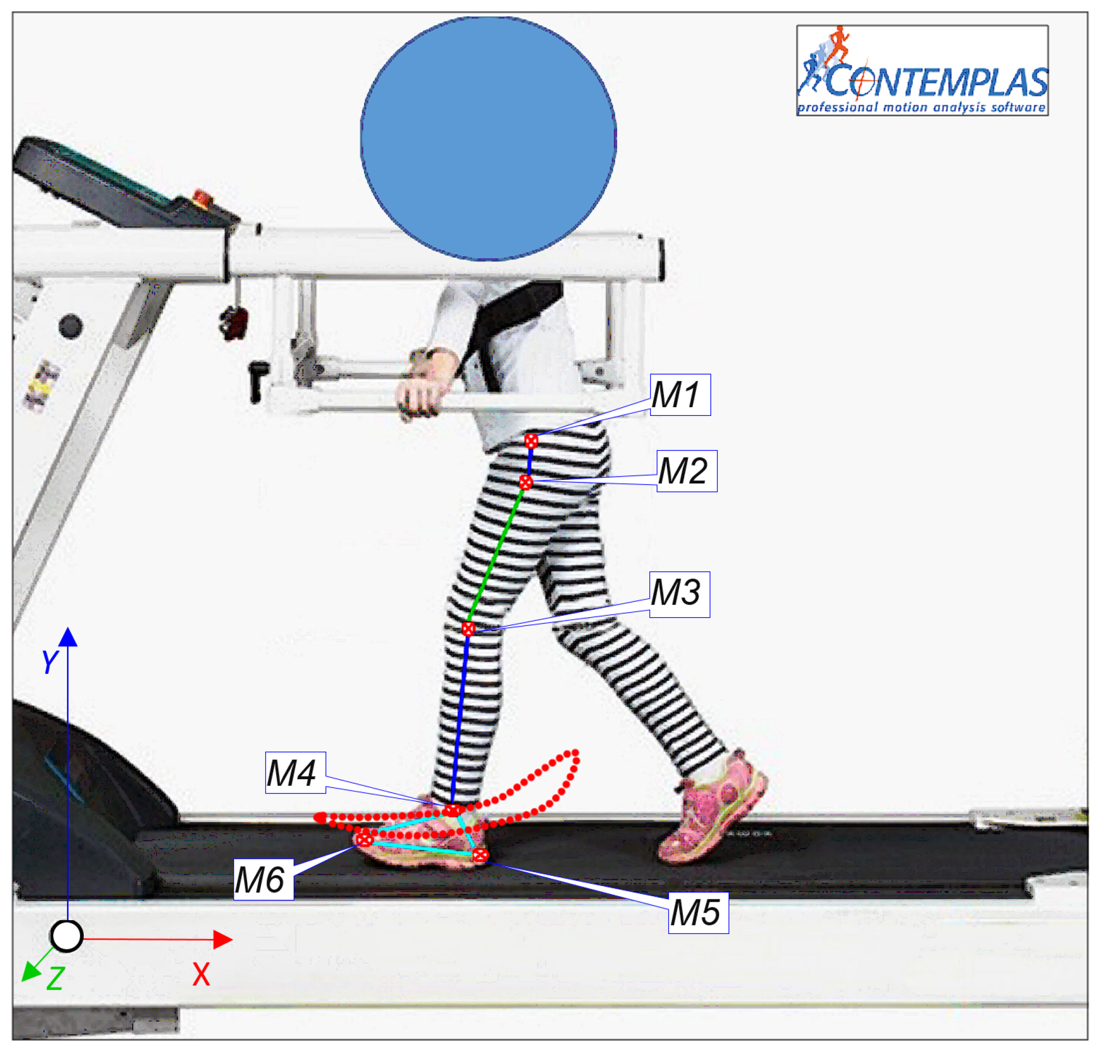
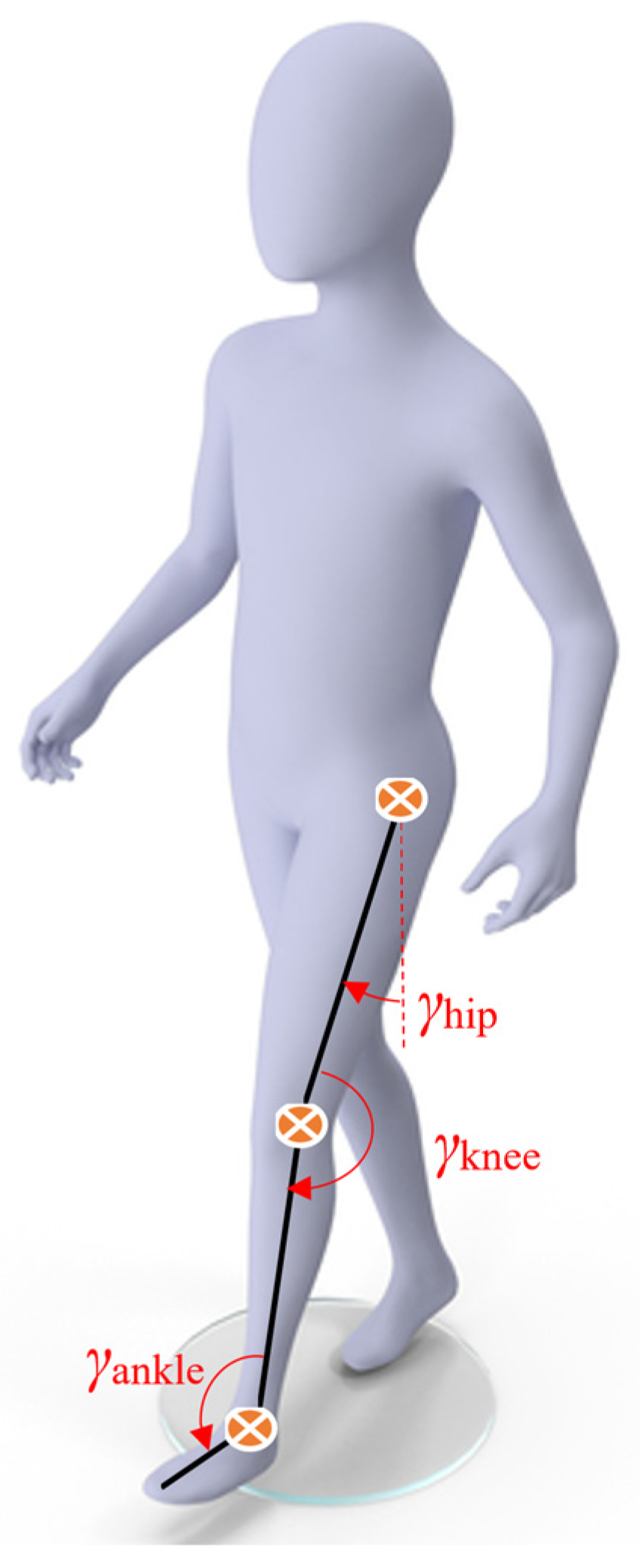
For the experimental analysis of walking activity, a four-year-old healthy child was chosen and the aim of this was to determine the hip, knee, and ankle joints motion laws and foot trajectory during a complete gait. For this analysis, a piece of equipment called CONTEMPLAS [
21] was used and the working principle of it was to track some specific markers attached to the human lower limb. These markers are reflective ones, and the software TEMPLO Motion 2016, associated with this equipment, has the ability to target and track these markers. The markers position was accomplished at the recommendations of a physician in order to identify each joint center position. The markers displacement can be seen in
Figure 1. According to
Figure 1, a set of 10 markers can be remarked and also a global coordinate reference system positioned on the treadmill frame. This position was also specified during equipment calibration to establish the correct values of the desired results.
In
Figure 1, the following notations can be identified: M1—pelvis mass center location; M2—hip joint; M3—knee joint; M4—ankle joint; M5—heel extreme point; M6—distal phalanges extreme point.
During a complete gait analysis, the child developed, at the level of the foot, a trajectory which is valuable for this research during experimental evaluation. This will be considered as a reference point for the desired trajectory of the designed leg exoskeleton. Also, this can be observed in
Figure 1. Two high-speed cameras with a speed of 350 frames/s recorded the human locomotion system motions. Both cameras were placed on the lateral side of the child in order to record each limb’s motion for a complete gait. Thus, the results developed by the left lower limb will be used for this experimental research. The interesting results are shown in
Figure 2,
Figure 3,
Figure 4 and
Figure 5.
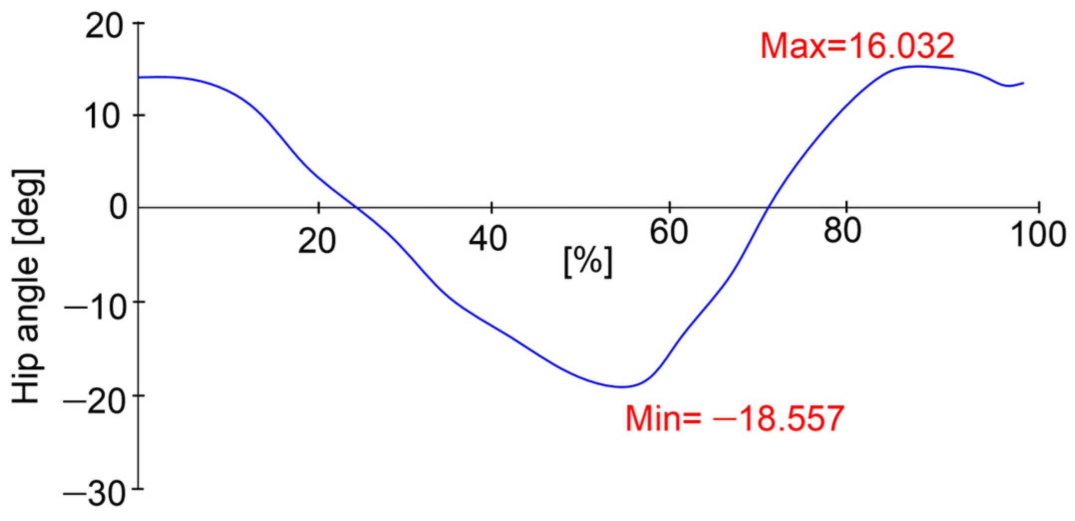
All experimental results were compared with the existing ones in the specific literature data, according to [
22], and the evaluated lower limb was the left one. By having in sight the reported plot from
Figure 2, it can be observed that the maximum value of the hip joint during a complete gait reached a maximum value of 16.03 degrees and a minimum value of −18.5 degrees. This means that the analyzed joint developed an angular amplitude of 34.5 degrees.
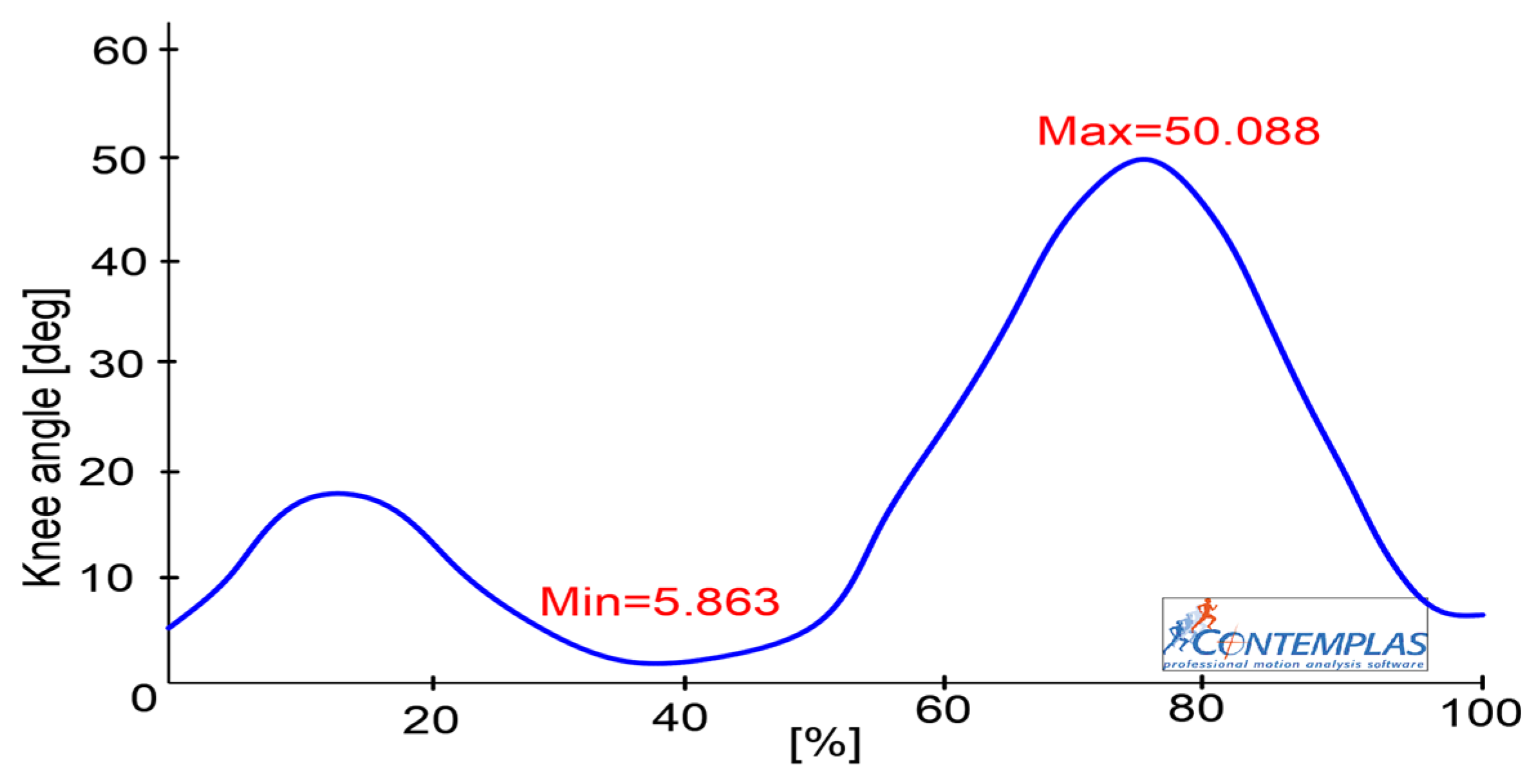
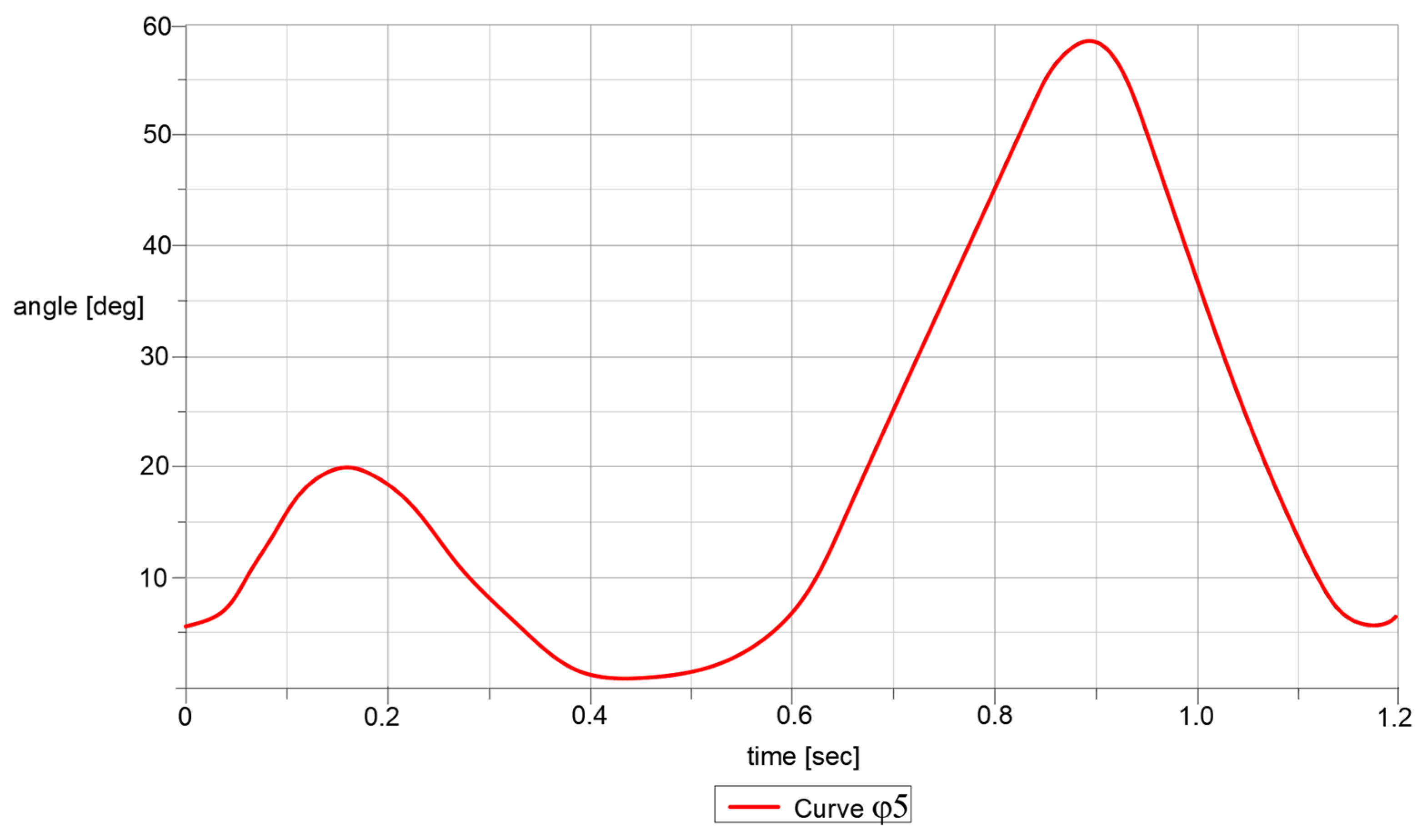
In the case of the knee joint, the obtained results are reported in the graph from
Figure 3. In the reported graph, it can be remarked that the maximum value of the knee joint flexion was equal to 50.08 degrees and a minimum one equal to 5.8 degrees. Thus, it resulted in an angular amplitude of the knee joint flexion equal to 44.2 degrees.
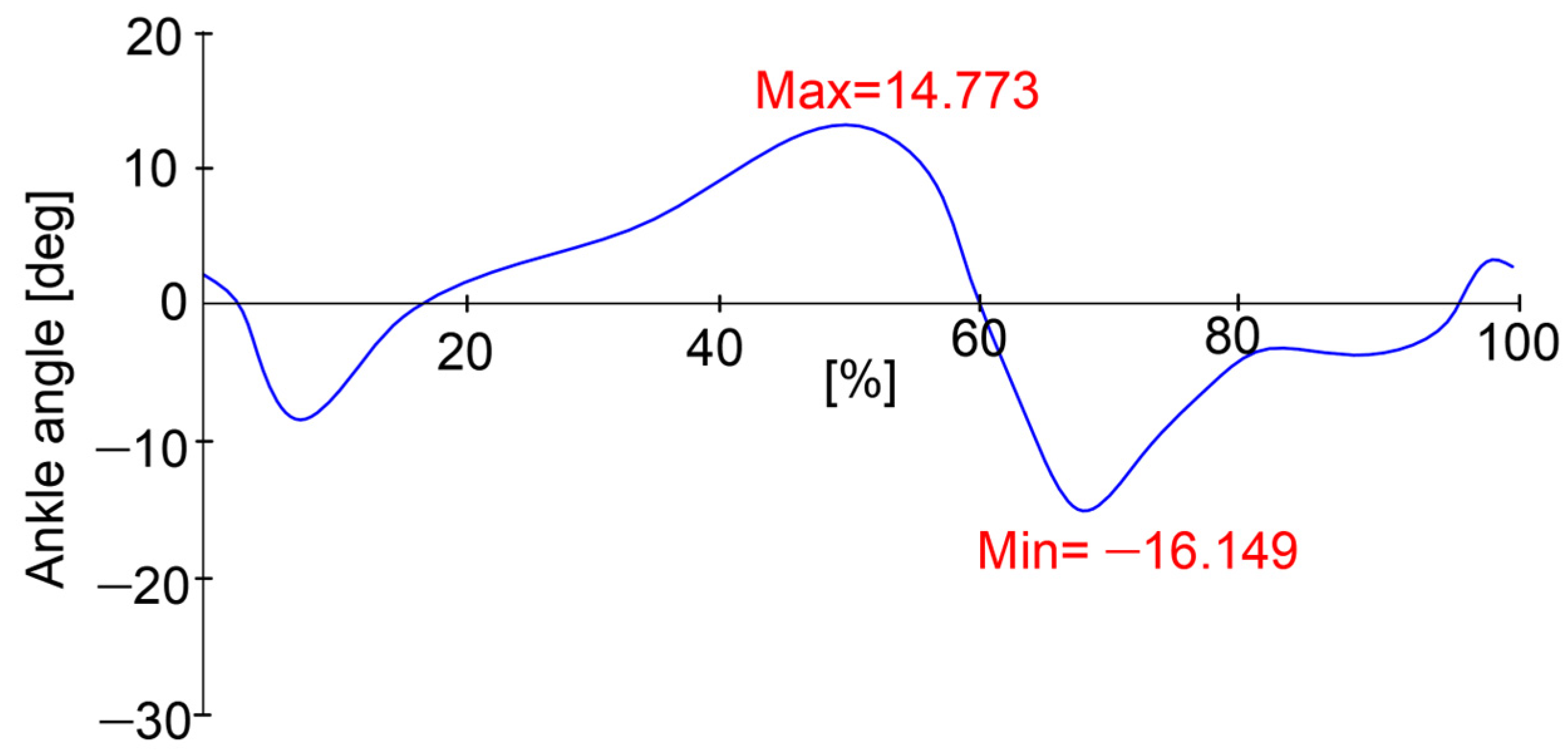
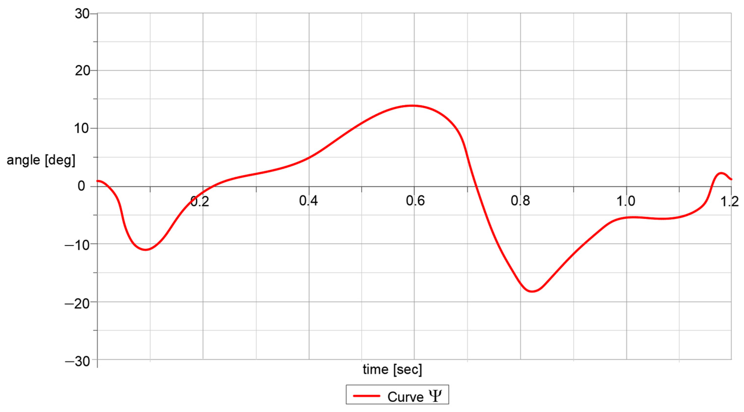
Simultaneously, the ankle joint was also analyzed and for dorsal/plantar flexions, a maximum value of 14.7 degrees, respectively, and a minimum one equal to −16.1 degrees, according to the reported plot in
Figure 4, were recorded. This means an angular amplitude equal to 30.9 degrees.
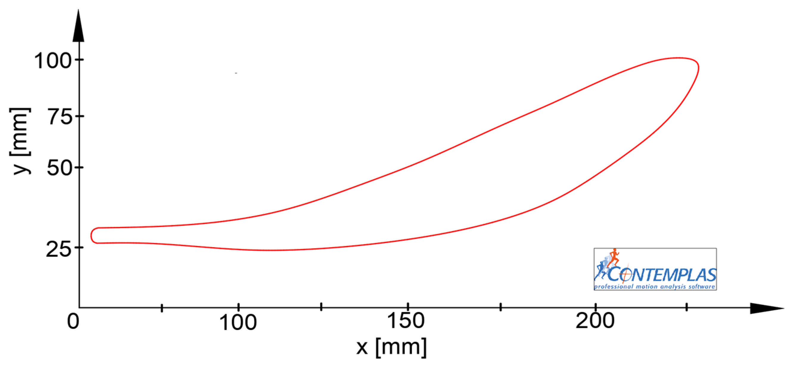
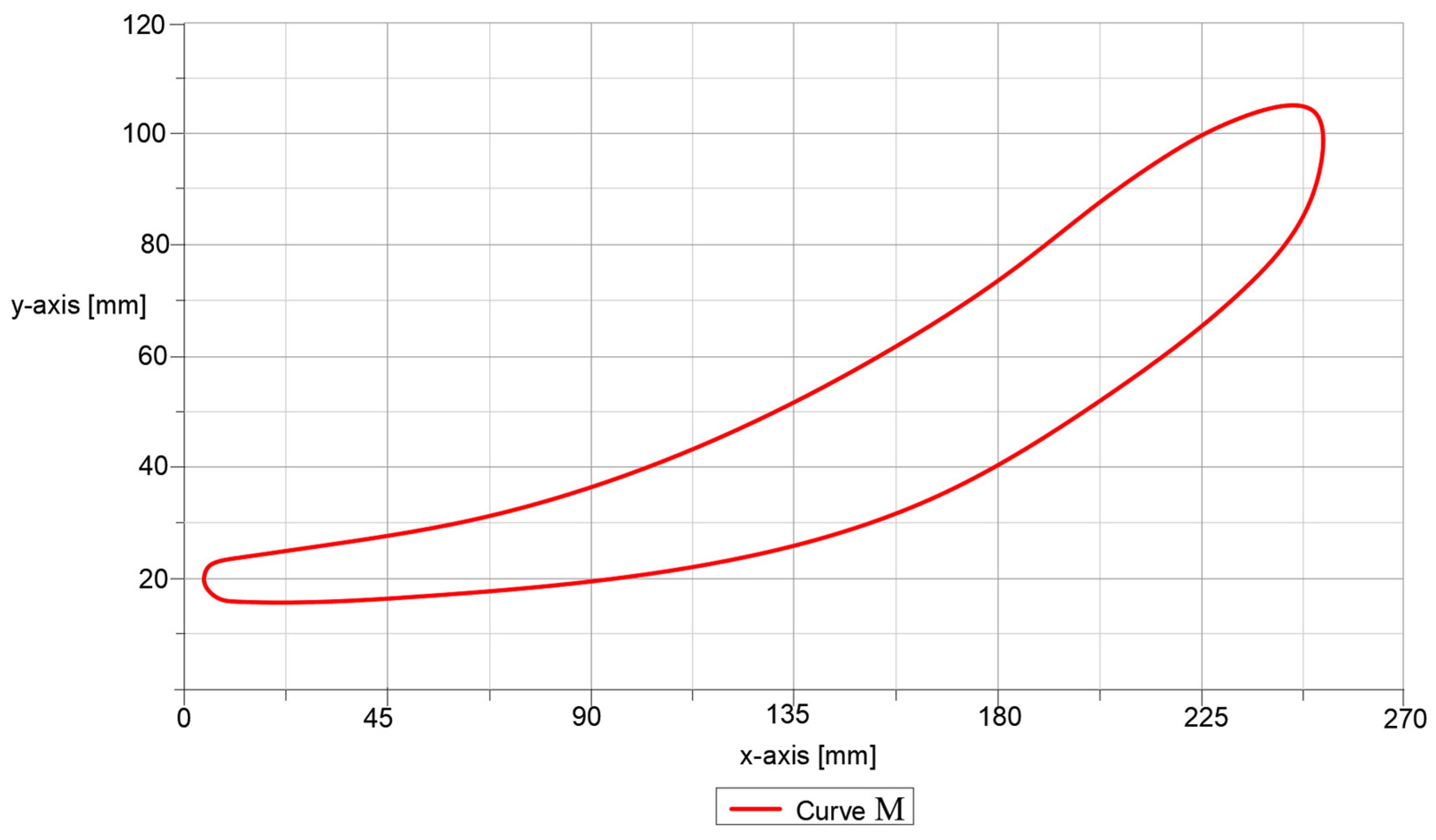
An essential experimental result was related to the M6—point foot trajectory, which is presented in
Figure 5. From this graph, the curve and the maximum and minimum values on x-y coordinates can be considered, in order to validate the proposed lower limb exoskeleton.
Furthermore, the experimental analysis gave the opportunity to evaluate the anthropometric data of the proposed human subject. Thus, the lower limb segment length was recorded, which will be used as input data for parametrizing the lower limb exoskeleton’s main dimensions. These dimensional parameters were Lfemur = 315 mm; Ltibia = 292 mm; Lfoot = 122 mm.
3. Conceptual Design of the Lower Limb Exoskeleton Mechanism
The design for a novel leg exoskeleton concept starts from previous solutions, namely a Chebyshev, pantograph, and cam mechanisms combination. The aim was to adapt a Stephenson III six-bar mechanism for ankle joint actuation extension. The reason for adapting this mechanism is given by the fact that this mechanism is an optimum solution that can assure lower limb trajectories required for gait rehabilitation purposes, as pointed out in [
19]. The mentioned mechanisms are represented in
Figure 7.
Some structural parameters of the solutions shown in
Figure 7 are listed in
Table 1, which are characterized by the mobility range.
Thus, the cam mechanism adapted for a leg exoskeleton design,
Figure 7b, gave a fair solution for elaborating a prototype, as reported in [
23]. The obtained leg exoskeleton solution from
Figure 7b was characterized by the cam-mechanism actuation for ankle joint motion and it had some disadvantages, like imprecise motions during overloads, a backlash between the cam follower and the cam body, and wear. This affected the gait phases through improper motions.
By considering the existent structural scheme from
Figure 7a and the general scheme of Stephenson III six-bar mechanism, from
Figure 7c, a new elaborated lower limb exoskeleton concept can be considered. From this, a structural scheme only to actuate the ankle joint, and to have a proper trajectory similar to the one reported in
Figure 5, was obtained. This adapted mechanism is shown through a structural scheme from
Figure 8.
The proposed solution combined the structural scheme of Stephenson III six-bar mechanism from
Figure 8 with the one presented in
Figure 7a. Thus, there will be two main parallel mechanisms, one for actuating hip and knee joints composed from Chebyshev and a pantograph mechanism combination, and the other only for actuating the ankle joint, namely Stephenson III six-bar mechanism, as can be seen in
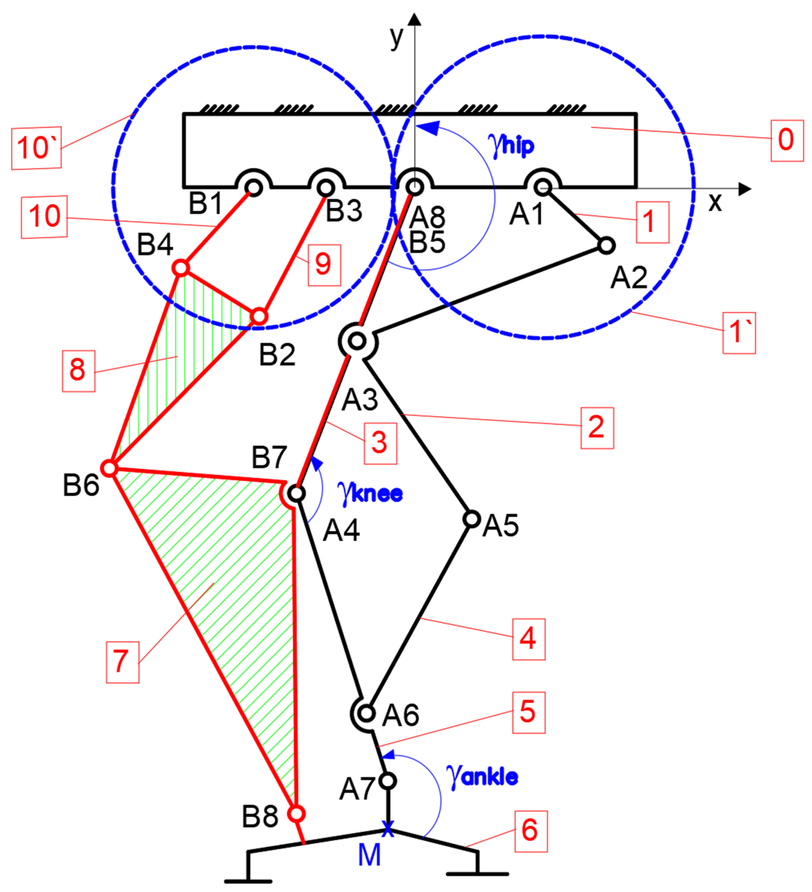
Figure 9.
From
Figure 9, it can be remarked that the drive link is no. 1 for actuating hip and knee joints under dictating angles γ
hip and γ
knee. Therefore, for the Stephenson III six-bar mechanism, the drive link was no. 1 according to the scheme from
Figure 8, but in the case of this parallel mechanism, the drive link will be substituted through the link no. 9 and will receive motion from a pair of gears, respectively, 10′ and 1′ with 1:1 ratio.
The mechanism functionality, based on the scheme in
Figure 9, was the following. The drive link 1 was fixed with the gear 1 and rotated through revolute joint A1 in accordance with the fixed frame 0. This actuated the Chebyshev mechanism through links no. 2 and 3 and the revolute joints A2, A8, and A3. In this way, link no. 3 equivalent to the femur will rotate with the angle γ
hip and the A8 revolute joint equivalent to the exoskeleton hip. On the other hand, the link no. 2 architecture is characterized by an angle of 90 degrees, which allows actuating the pantograph linkage made from links no. 2, 4, and 5, respectively, revolute joints A3, A4, A5, and A6. Thus, link no. 5 is equivalent to the tibia segment and it connects to link no. 3 through revolute joint A4, which is equivalent to the knee joint and this rotates with the angle γ
knee. For actuating the ankle joint, the Stephenson III six-bar mechanism placed in parallel with the other one will be used. For this, the motion is received from gear no. 10′ which is fixed with link no. 10. This link will actuate the first part of the mechanism linkage through the revolute joints B1, B4, B2, B3, and B6. The revolute joint B6 is common with the second part of the linkage, namely links no. 7, 6, and 3. This part is characterized by the revolute joints B6, B7, B8, and B5. One remark is that link no. 3 is common for both mechanism linkages and corresponds to the femur segment. Link no. 7 will actuate with a proper motion angle γ
ankle the revolute joint A7, and link no. 6, respectively, point M will describe an imposed trajectory as the one reported in
Figure 5.
Thus, the mobility range is equal to one due to 10 links, 28 revolute joints, and a pair of gears. The entire linkage from
Figure 9 will be considered as a starting point for further kinematic and dynamic analyses.
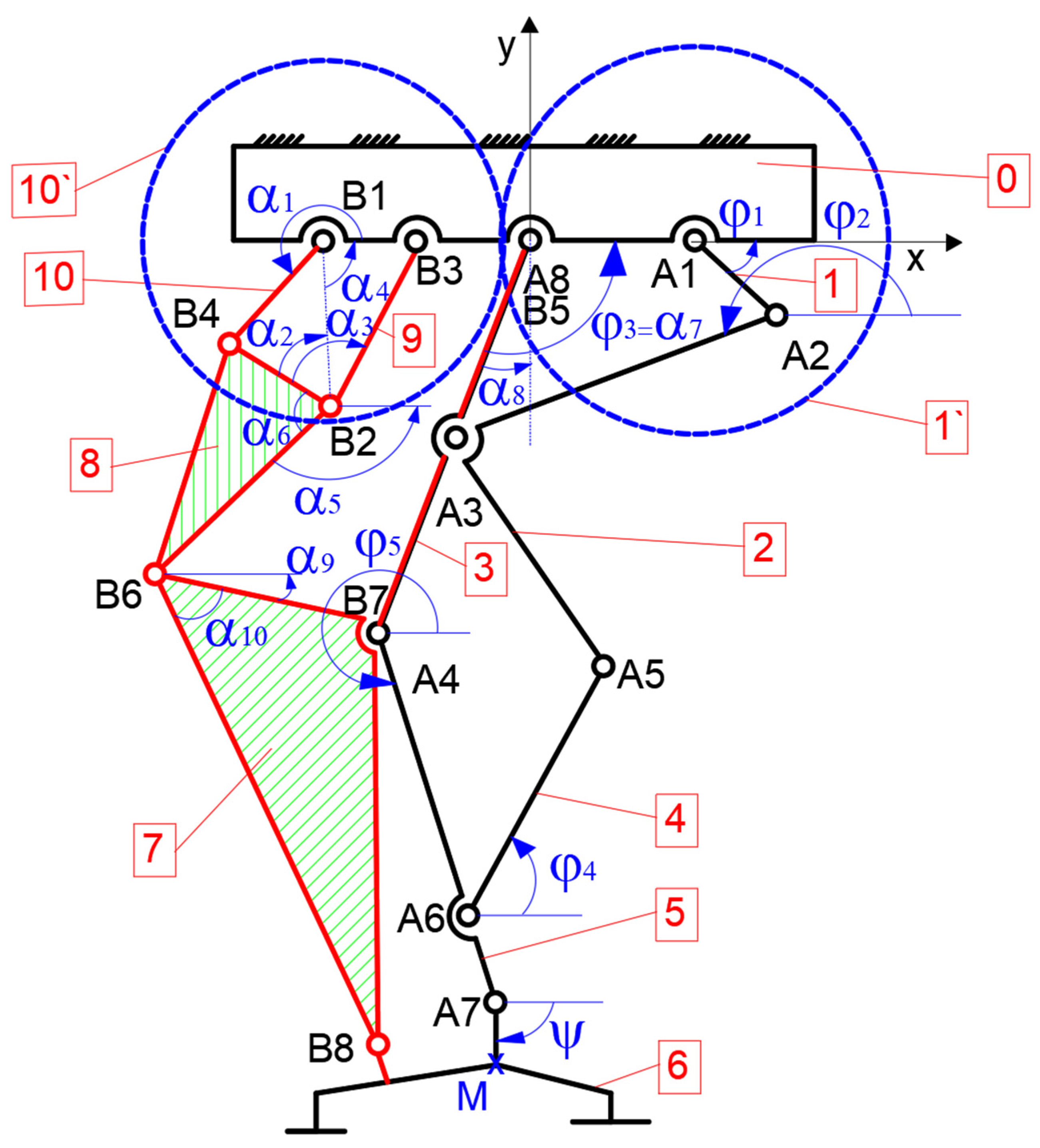
4. Kinematic Analysis
For the kinematic analysis of the novel lower limb exoskeleton, a kinematic scheme was elaborated, in accordance with the structural scheme presented in
Figure 9, as can be seen in
Figure 10.
The aim of this analysis was to determine the angular positions of the target equivalent joints, namely hip, knee, and ankle. Another objective was to obtain a proper M-point trajectory, similar to the one presented in
Figure 5.
The mathematical model elaborated in this section was a parametrized one, which allowed us to adjust the proper main dimensions similar to the ones of the child used in the experimental analyses frame.
From
Figure 10, two parallel mechanisms can be observed, namely an adapted Stephenson III six-bar mechanism for ankle joint actuation, and another one composed of a Chebyshev and a pantograph linkages for actuating hip and knee joints.
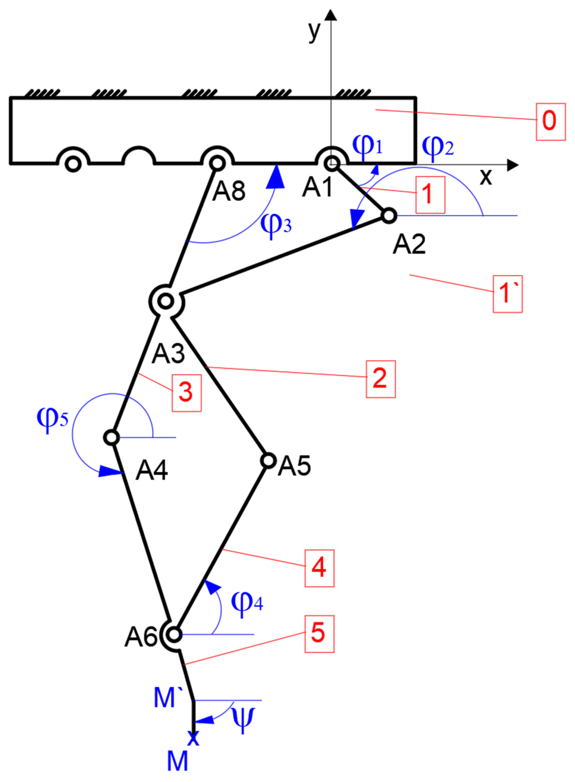
4.1. Chebyshev and Pantograph Mechanism Kinematic Analysis
The kinematic model of the proposed mechanism is shown in
Figure 11, and the obtained equations will demonstrate the performance and operations for hip and knee joints.
From
Figure 11, the local coordinate system is located in the A1 revolute joint. The following convention of the angle notation holds: φ
3 = γ
hip and φ
5 = γ
knee.
The point A4 position can be calculated as a function of the drive link angle φ1, in accordance with the XOY reference system, and the kinematic parameters of the Chebyshev linkage O, A2, A8, and A3.
Thus, the position of point A3 can be evaluated in accordance with the local coordinate system by
The position of
M′-point, according with the base frame 0 can be given as
In this way, point
M position can be calculated by
If it needs to evaluate velocities for points A8,
M′, and
M, Equations (1)–(3) and the angles
φi (with
i = 1 to 5) can be solved by considering the closure loops equations as a function of
φ1 =
ω·
t to give
where:
The M-point acceleration can be obtained the following mathematical expressions
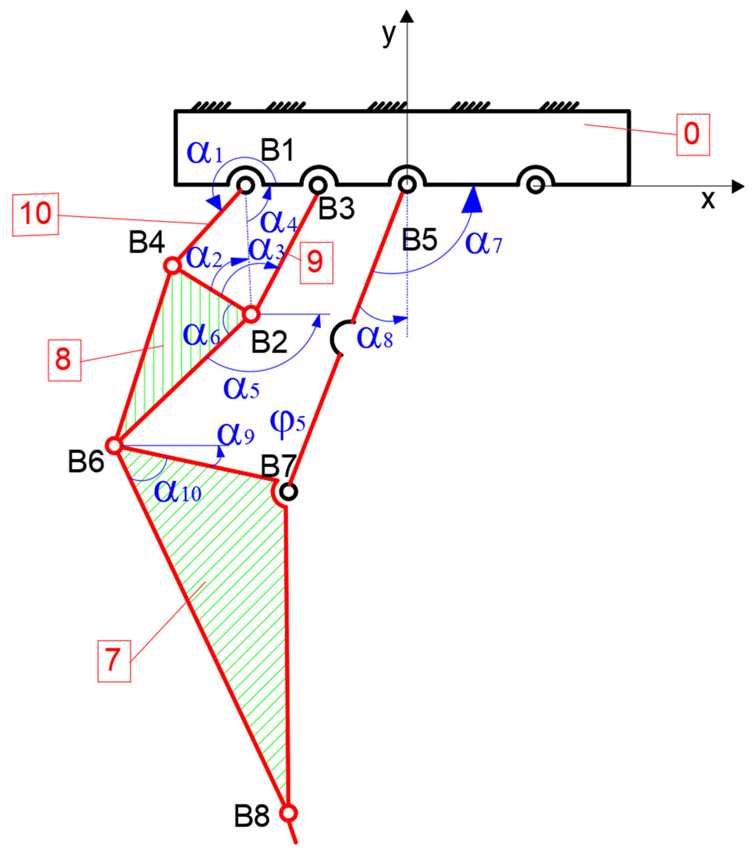
4.2. Stephenson III Six-Bar
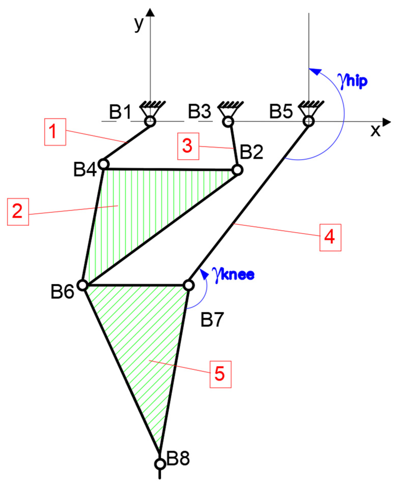
According to the kinematic scheme in
Figure 10, the second mechanism linkage which actuates the ankle joint is shown separately, in
Figure 12. A similar research was developed in [
19].
From
Figure 12, it can be seen that B1 was located at the level of the local coordinate system origin, B3 and B5 were revolute joints under the base frame.
Thus, the joints B5, B7, and B8 matched to the hip, knee, and ankle joints. This kinematic model had one actuator, namely the drive link no. 1 which will receive motion through a pair of gears namely 1 and 9′.
By calling at analytical geometry, it is necessary to differentiate each joint position based on the assumed angles (αk with k = 2 to 10) in accordance with the input angle α1.
These angles and the distances between the revolute joints can be differentiated and represented by Equations (10)–(15).
Thus, the positions of the mechanism characteristic points in accordance with the drive link angle α
1 can be computed by
To compute velocities or accelerations, these can be obtained from successive differentials of Equations (16)–(20).
4.3. Numerical Processing
A kinematic analysis can be carried out by creating an algorithm under MAPLE software R12 environment for computing the kinematic models, which were previously presented. For this, it is necessary to have the length links of the mechanism presented in
Figure 10 in numerical form. These values were obtained by taking into account the anthropometric data of the child, considered as reference positions.
Thus, for the first mechanism linkage, the following input data were considered: lA1A2 = 25 mm; lA2A3 = 222.5 mm; lA4A8 = 305 mm; lA3A5 = 225 mm; lA5A6 = 240 mm; lA4M = 292 mm.
For the second mechanism, the input data are lB1B4 = 25 mm; lB2B3 = 65 mm; lB4B2 = 85 mm; lB2B6 = 112.65 mm; lB5B7 = 305 mm; lB6B7 = 15.6 mm; lB6B8 = 243.54 mm; lB7B8 = 323.5 mm, lB4B6 = 115.15 mm.
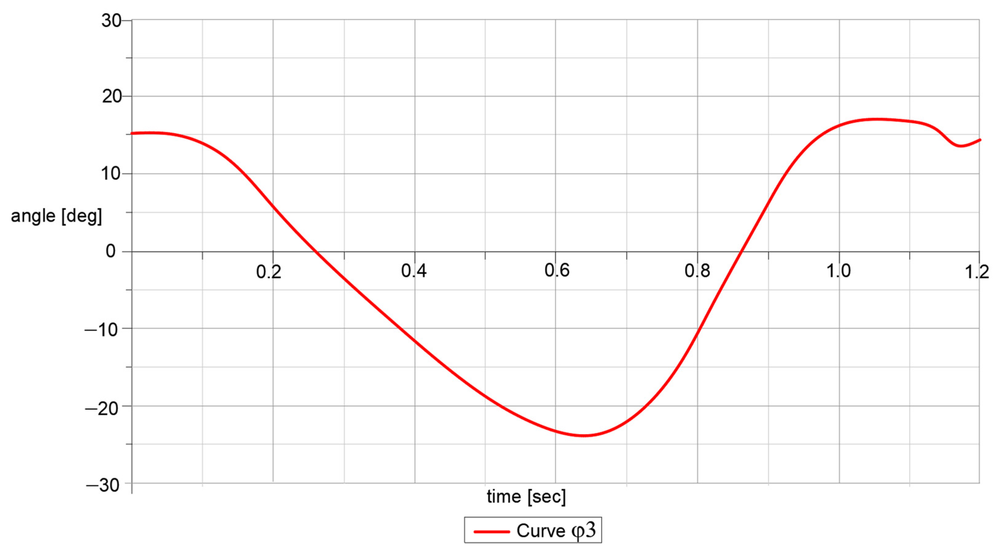
Thus, by processing the input data, numerical results have been obtained without considering the lower limb exoskeleton touching the ground. The targeted results are characterized by the angular positions of the hip, knee, and ankle joints. Also, the M-point trajectory under the x-y coordinate system represents an important result of performance characterization. These results are represented through the diagrams in
Figure 13,
Figure 14,
Figure 15,
Figure 16 and
Figure 17.
By having in sight these graphs reported in
Figure 13,
Figure 14,
Figure 15,
Figure 16 and
Figure 17, it can be observed that the obtained results are similar to the ones obtained throughout experimental tests, with a human participant. In addition the computational algorithm cannot be used in terms of a complete gait as 100%, and for this, the time function was chosen, which for a complete gait, the child used in experimental tests performs in 1.2 s. In the case of M point trajectory, this was computed from two components, namely
x-axis component and
y-axis component, as a function of time. After this, the numerical results were extracted and combined in another graph, i.e., the one in
Figure 16.
5. CAD Design and Numerical Simulations
5.1. Lower Limb Exoskeleton Virtual Simulations
By having in sight the structural and kinematic schemes in
Figure 9 and
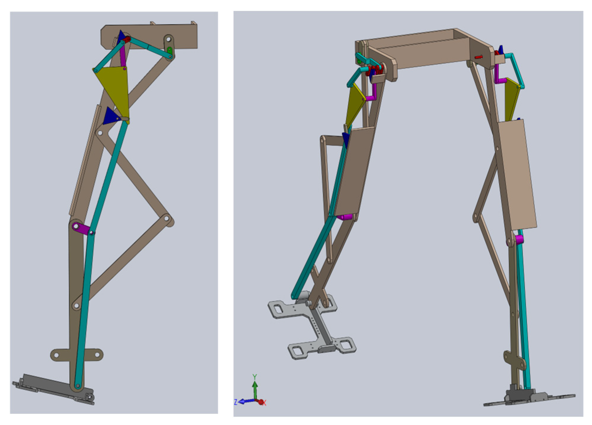
Figure 10, and considering the dimensions used during numerical processing, a CAD model was created in a simplified parametrized form with the aid of SolidWorks software 2016. This lower limb exoskeleton model is shown in
Figure 17, and it was created in a mirror position in order to have both legs. The aim of designing this was to better characterize the results from the kinematic analysis developed in the previous section.
An interface was created for exporting the CAD model, under the extension of a Para-solid file, to MSC ADAMS/Adams View software version R17 module. During virtual simulations, foot–ground contact was neglected. Also, the virtual model setup under the Adams View interface was made in accordance with data from [
24].
The whole linkage was considered as made from aluminum alloy type 1060, with the following main characteristics: Elastic modulus—69,000 N/mm2, Poisson ratio—0.33, Mass density: 2700 kg/m3, Tensile strength: 68.9356 N/mm2.
There were defined 59 revolute joints, by taking into account the friction with the following data: static coefficient—0.01, dynamic coefficient—0.0025, pin radius of the ball joints—0.95 mm, stiction transition velocity—0.1, maximum stiction deformation—0.01.
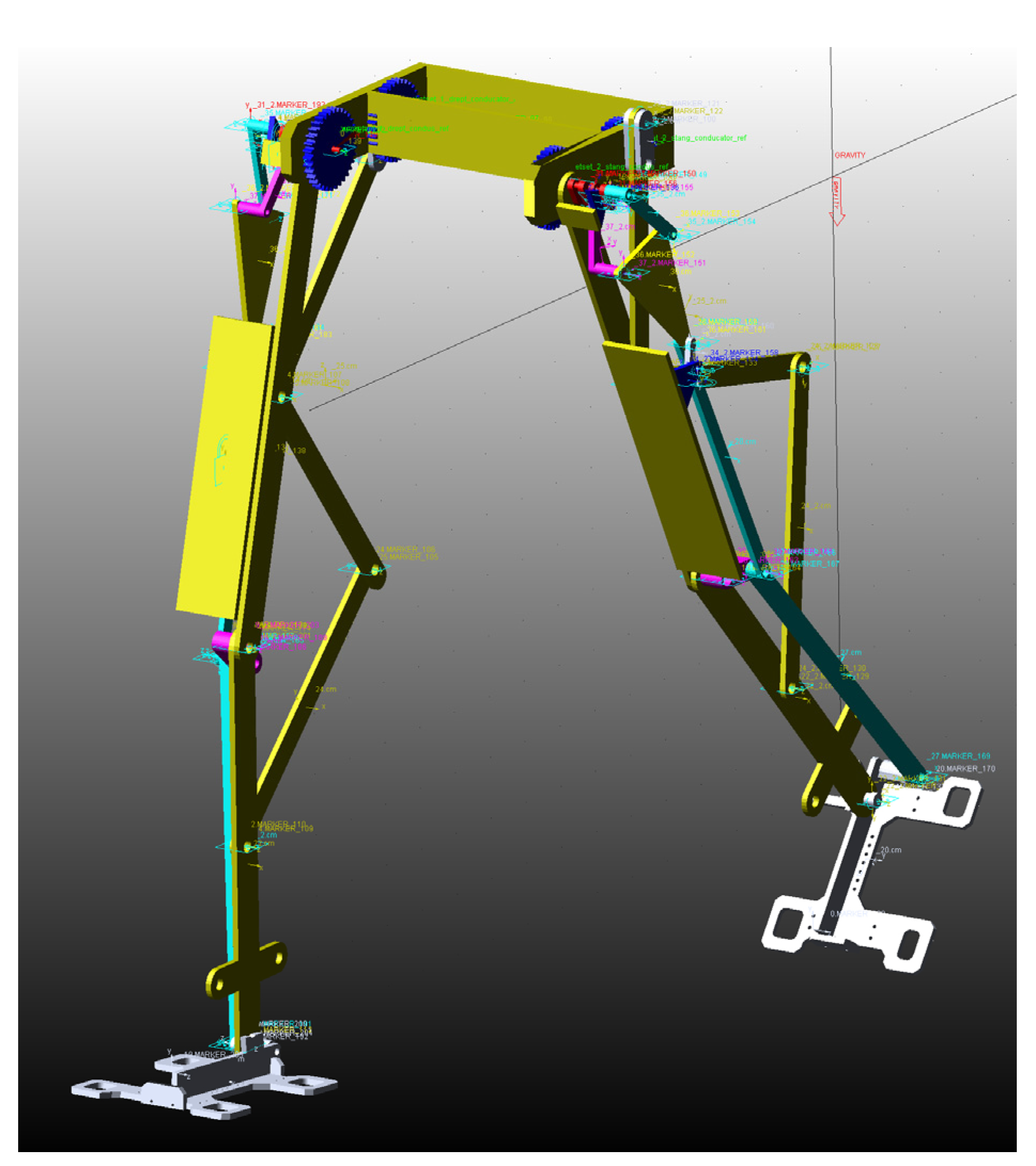
Figure 18 shows the imported exoskeleton model under MSC Adams environment, where the defined revolute joints and links identification can be seen.
For simulations, initial conditions were considered like the ones for the child used in the experimental analysis frame. Thus, the exoskeleton linkage was placed in a biped position when the left lower limb start the gait phases, and the right one finished the gait phases, and these were in a close-loop action. The time period used in simulations was also defined and this was equal to 1.2 s, which corresponds to a complete gait.
A proper actuator was defined under the drive link no. 1 (which corresponds to Chebyshev and pantograph mechanism), and for actuating the Stephenson III six-bar mechanism it was defined as a pair of gears with a 1:1 ratio.
The actuator will rotate under a motion function depending on time and angular displacement (30 degrees*time), and the gears, there were considered the following parameters: gear width—8 mm; teeth number—33; axis center—85 mm; tooth angle—15 degrees; material—steel.
For the simulations, a GSTIFF solver with a defined error of 0.001 was used.
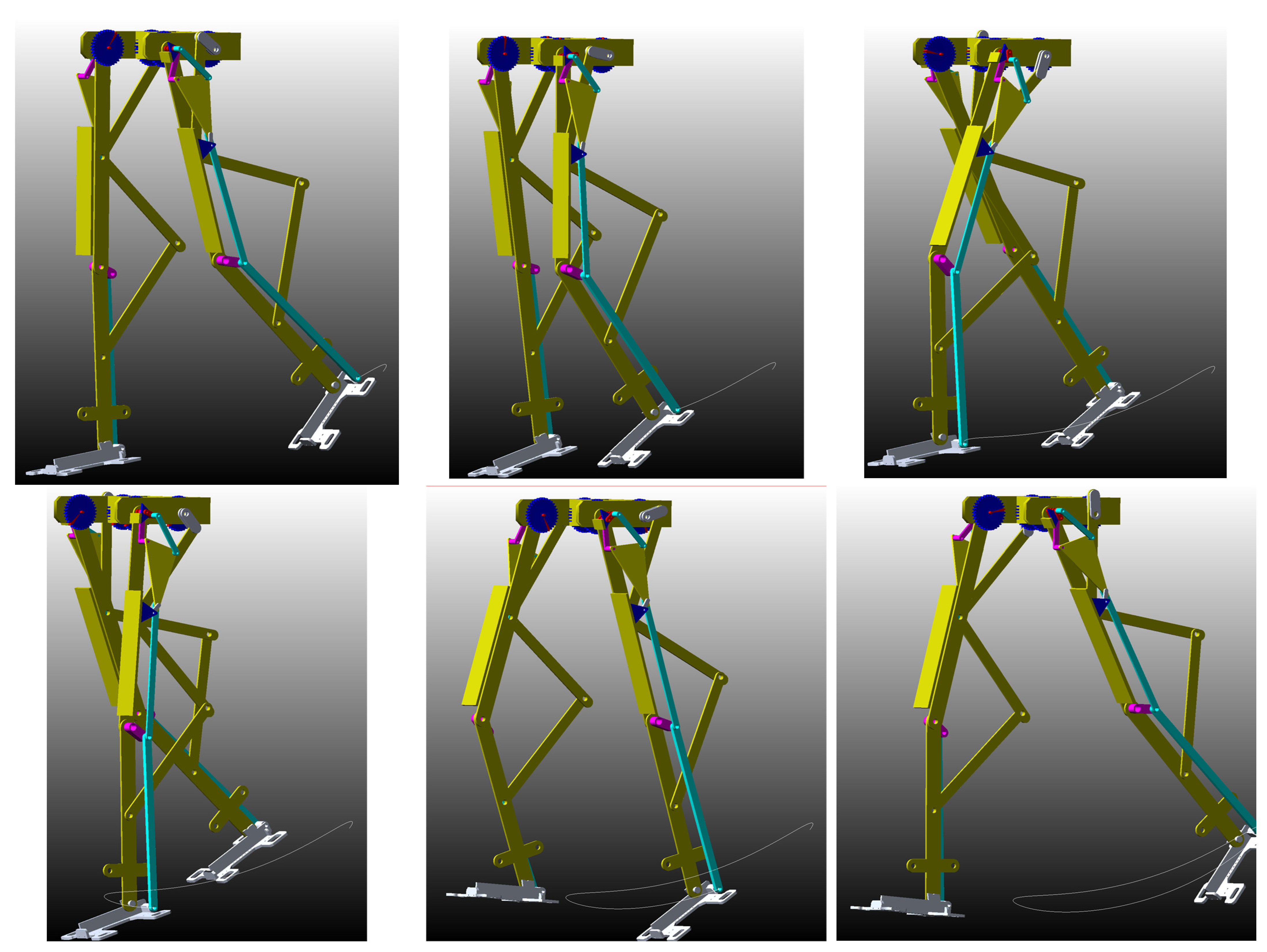
Thus,
Figure 19 shows snapshots during a complete gait, and the snapshots were characterized by M-point trace and generating the specific trajectory.
Simulations were processed in order to determine the feasibility of the lower limb exoskeleton design and to characterize its operation features. Thus, the obtained results were represented by motion laws for the left hip, knee, and ankle joints. Obviously, the M point trajectory data were also obtained. These results were obtained in a numerical form, in order to perform a comparative motion analysis, as discussed in the next section.
5.2. Results and Discussions
A comparative analysis was performed by using the numerical values of the obtained result, from experimental tests, kinematic model processing, and simulations under MSC Adams version R17 software.
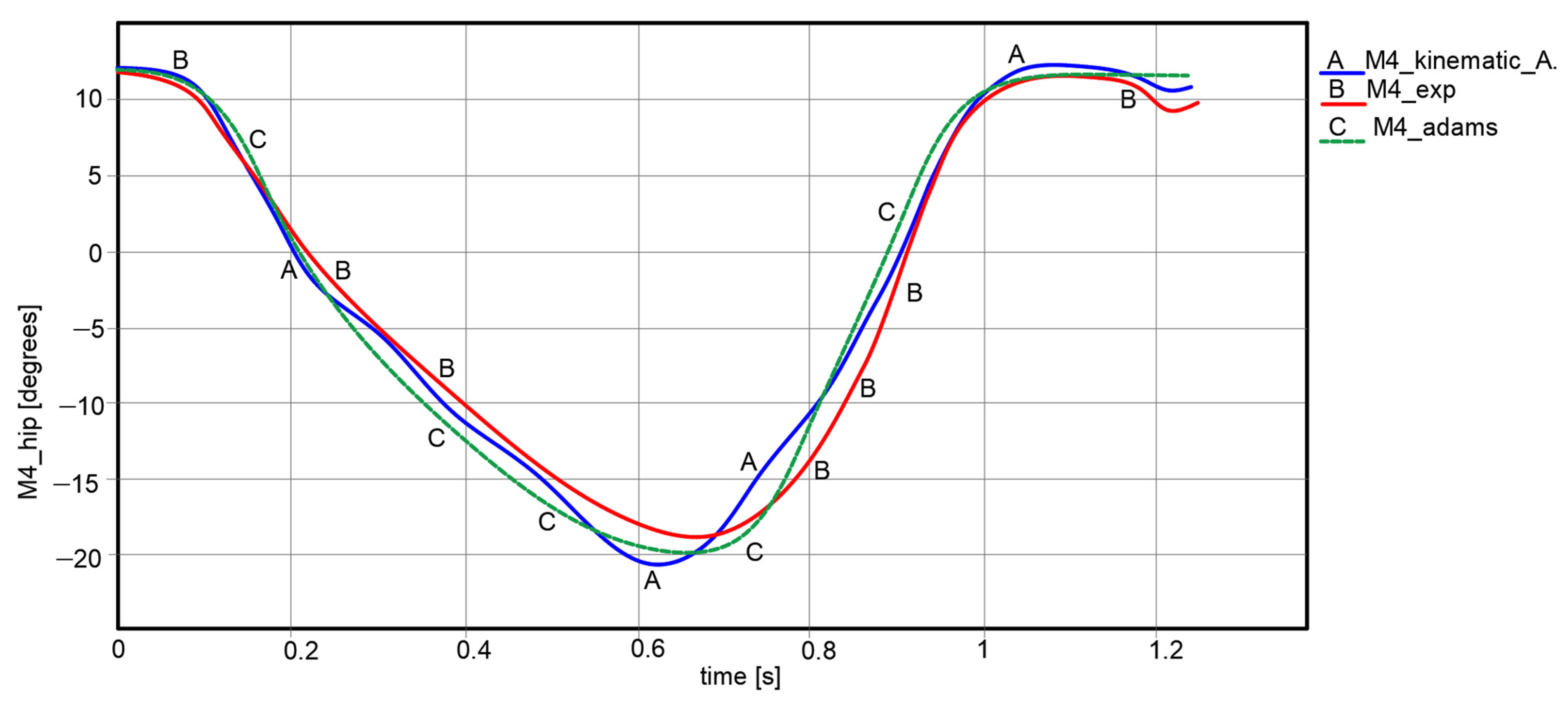
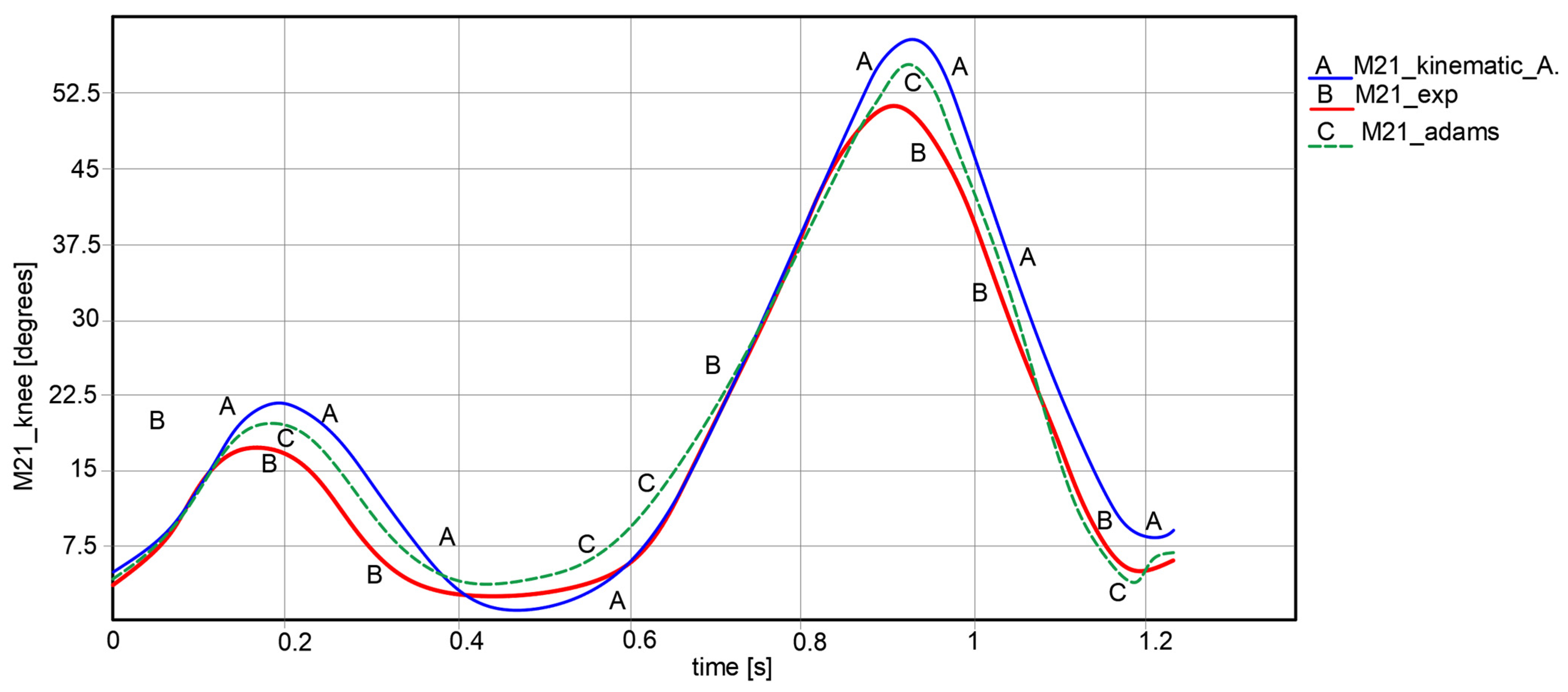
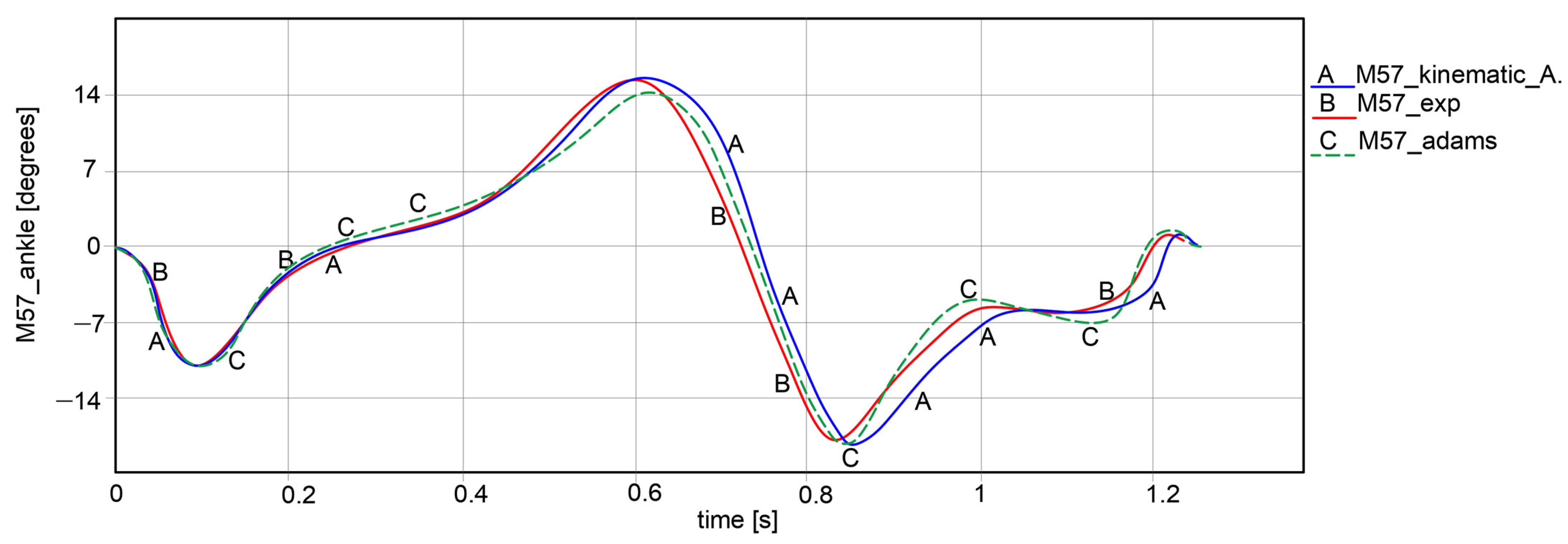
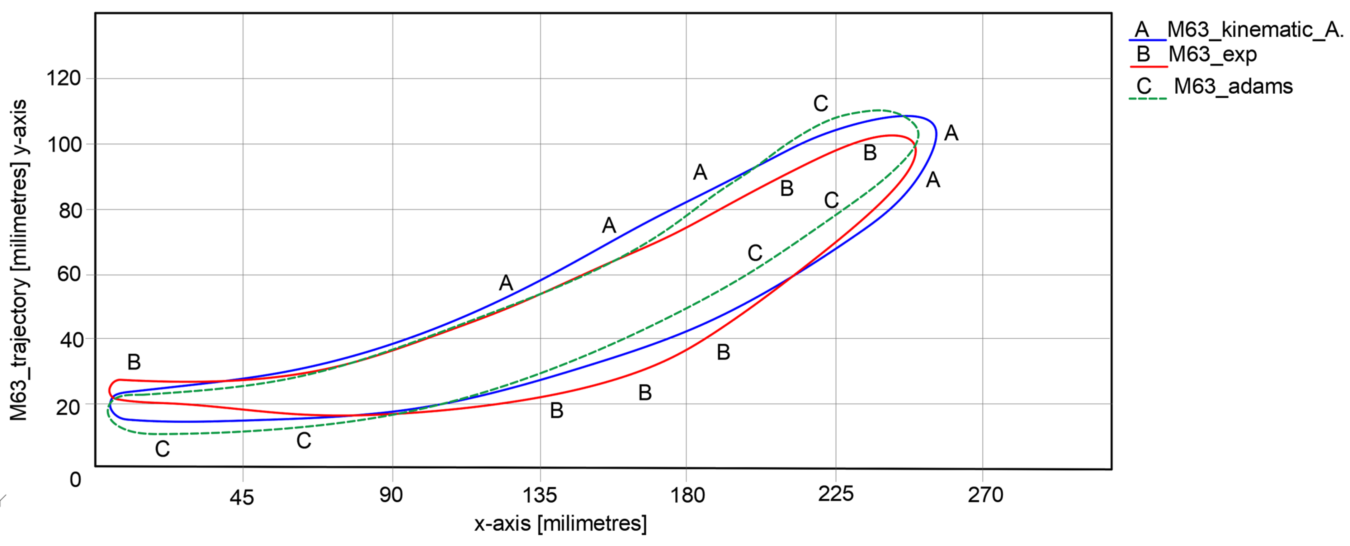
For this, a specific import interface under LS-Dyna software version R12 was used in order to calculate the accuracy of the obtained results. At the beginning, for the input data, correspondence between notations was made. Thus, M4—point corresponds to the hip joint rotation center, namely γhip = φ3; M21—point corresponds to the knee joint rotation center, respectively γknee = φ5; M57—point corresponds to the ankle joint rotation center, namely γankle = ψ. In the case of the foot trajectory, the correspondence was M67—point is M6—point from experimental analysis section and M—point from kinematic analysis section.
The input values were also filtered by using FFT filtering algorithm. In this way, results were obtained as the four plots reported in graphs in
Figure 20,
Figure 21,
Figure 22 and
Figure 23.
Using these diagrams, and with the aid of Ls-Dyna software version R12 module, maximum and minimum values were extracted, which are summarized in
Table 2. Another reason for calling LS-Dyna module is that this program can estimate data accuracy for each obtained graph. The established accuracy is also indicated in
Table 2.
An important note for the plots reported in
Figure 20,
Figure 21,
Figure 22 and
Figure 23 is the one that the paths were appropriate one to another for all cases, respectively, experimental tests, kinematic analysis, and simulations with Adams software version R17.
By having in sight the reported numerical values extracted from LS-Dyna, it can be remarked that the maximum numerical value of less accuracy reached a value of 4.48% in the case of knee joint motion law. High accuracy was obtained in the case of ankle joints, respectively, a minimum numerical value of 1.61%. This represents that the Stephenson III six-bar mechanism had good behavior in a combined solution with the other two mechanisms. The whole lower limb exoskeleton average accuracy was 2.884%, and this value was under 5%, which represents the maximum accuracy value for validating the lower limb exoskeleton solution.

 ,
, 


