Intelligent Tool-Wear Prediction Based on Informer Encoder and Bi-Directional Long Short-Term Memory

Abstract

Herein, to accurately predict tool wear, we proposed a new deep learning network—that is, the IE-Bi-LSTM—based on an informer encoder and bi-directional long short-term memory. The IE-Bi-LSTM uses the encoder part of the informer model to capture connections globally and to extract long feature sequences with rich information from multichannel sensors. In contrast to methods using CNN and RNN, this model could achieve remote feature extraction and the parallel computation of long-sequence-dependent features. The informer encoder adopts the attention distillation layer to increase computational efficiency, thereby lowering the attention computational overhead in comparison to that of a transformer encoder. To better collect location information while maintaining serialization properties, a bi-directional long short-term memory (Bi-LSTM) network was employed. After the fully connected layer, the tool-wear prediction value was generated. After data augmentation, the PHM2010 basic dataset was used to check the effectiveness of the model. A comparison test revealed that the model could learn more full features and had a strong prediction accuracy after hyperparameter tweaking. An ablation experiment was also carried out to demonstrate the efficacy of the improved model module.

1. Introduction

The year 2025 will see the implementation of smart manufacturing; the traditional manufacturing industry has been gradually upgrading to intelligent manufacturing, and an increasing number of intelligent machines and pieces of equipment are being used in the manufacturing industry [1]. Tool-wear condition during machining is an essential element in guaranteeing the dependability and stability of the manufacturing process [2]. Previous studies have shown that the downtime of a machine tool caused by severe tool wear accounts for 15–40% of its total downtime, with the actual service time of the tool only accounting for 60–80% of its full service life [3]. Early warnings of tool wear can lead to higher production costs, lower profits, and wasted productivity [4]. Nonetheless, tool-condition monitoring can be expected to reduce machine downtime by up to 75%, and by simply offering useful tool-usage advice, productivity can be increased by at least 65% [5]. Therefore, it is crucial to accurately predict the tool-wear state in order to ensure production quality, to cut costs, to boost productivity, and to prevent serious safety incidents. Widespread interest in the field of tool-condition monitoring research has been sparked by the advent of data-driven models, made possible by the rapid advancement of artificial intelligence and big data.

Direct measurement [6] and indirect measurement [7] techniques can be used to monitor tool wear. Direct measurement methods cannot obtain real-time detection. Consequently, with the development of advanced sensor technology, most methods today involve indirect measurements, collecting relevant data through one or more sensors, such as Hall, acceleration, cutting force, and acoustic emission sensors.

By building an appropriate data-driven model, it is possible to establish the mapping link between the measurement data and the tool-wear condition. Traditional machine learning techniques have been employed in past studies to forecast tool wear. Machine learning techniques can be used to determine the nonlinear mapping relationship between cutting signals and tool wear. These algorithms comprise the support vector machine (SVM) [8,9], the hidden Markov model (HMM) [10,11,12], the artificial neural network (ANN) [13,14], the random forest, and the Gaussian process regression (GPR) algorithms [15].

For example, support vector machines and the gray wolf optimization algorithm were used by Liao et al. to predict tool wear [16]. Dong et al. [17] used Bayesian support vector machines to extract features from force signals for tool-wear forecasts. Wang et al. [18] used an HMM to monitor tool wear during machining. Palanisamy et al. [19] used regression mathematics and an ANN to monitor tool wear. However, the extraction of these statistical traits necessitates expert knowledge and abilities in the relevant domains. In the age of manufacturing powered by big data, with the ensuing explosive growth in monitoring data, it has become difficult for engineers to manually extract features from the massive volumes of raw data. These experience-based feature extraction algorithms are still challenging [20]. Additionally, the traditional method model is small in scale and weak in generalization ability, making it difficult to adapt to complex and changeable processing scenarios. As a result of rapid computer science and technology improvements, deep learning methods are now widely used in many different industries. With a strong generalization ability, deep learning is suitable for processing massive volumes of original data and can adaptively extract the relevant features from training data. Therefore, tool-wear state identification combined with deep learning models has become a hot topic in the industry and has attracted wide attention.

Currently, tool-wear status monitoring based on deep learning includes the use of recurrent neural networks (RNNs) [21], convolutional neural networks (CNNs) [22], and autoencoders (AEs) [23]. The RNN model uses a shared parameter network in which all network parameters are shared across all time steps by scanning the input data such that each time step has access to both the current time’s input and the past time’s output, enabling the model to successfully use past input information to assist it during the current time. For example, the long short-term memory network (LSTM) was used by Marani et al. to track tool-wear status [24]. Zhang et al. used densely connected CNNs and gated RNNs to monitor tool-wear condition [25]. Using convolution and pooling layers, the CNN model can extract and screen the sensitive features hidden in an input feature map and use them to achieve a preset goal. For example, Cao et al. [26] used a two-tree complex wavelet transform and a CNN to accurately determine the degree of tool wear. Cutting force and vibration data were used by Huang et al. [27] to extract time-domain, frequency-domain, and time-frequency domain features and to develop CNNs in order to achieve tool-wear prediction.

Currently, the combination of CNN- and RNN-based models is the method of choice in the field of tool-wear monitoring. For example, for the purpose of tool-condition monitoring, Cheng et al. [28] developed a parallel CNN structure with several layers, which was then followed by bi-directional long short-term memory (Bi-LSTM). According to the 1D-CNN and Bi-LSTM models, Bazi et al. [29] used a combination of CNN and Bi-LSTM models for tool-condition monitoring. Both models showed strong temporal and spatial feature extraction capabilities, but they still exhibited several shortcomings in the face of long input-sequence prediction scenarios. Models such as CNN-based models generally solve the problem of long-distance feature capture by stacking convolutional layers; however, this approach cannot ensure that the model effectively extracts long-distance features, and the computational efficiency may suffer from the large number of model parameters.

RNN-based models—such as the LSTM and GRU—have achieved good results in scenarios with a limited input range, but they are restricted by the RNN’s sequence-dependent structure, which can make it hard for the RNN to career progression parallel computing ability. At present, the modification of CNN- and RNN-based models—including the introduction of residual structures, attention mechanisms, and multi-scale fusion—can improve their performance to a certain extent, but the characteristics of the network model limit their ability to establish long-distance time-series features.

In view of the shortcomings of CNN- and RNN-based models, a transformer model was proposed by Vaswani et al. [30]. The entire network structure of the transformer model comprises an attention mechanism and a feedforward neural network. The transformer model has been a great success in natural language processing, effectively solving the long-sequence prediction problem. As a consequence, it has been employed by numerous academics in the field of fault diagnosis and prediction. For instance, Liu et al. [31] proposed a transformer-based model of neural networks for tool-wear monitoring. However, the transformer was composed of multiple self-attention stacks, too many of which could lead to too many variables consuming too much memory. In addition, self-attention, one of the transformer’s essential elements, doubles each layer’s computational difficulty as the length of the sequence increases via the dot-product operation.

In response to these problems, Zhou et al. [32] proposed the informer model, which uses the prob-sparse self-attention mechanism to reduce the complexity of the dot-product calculation from quadratic to linear growth, thus reducing computational complexity. Moreover, when the input sequence is long, information may not be very concentrated. Zhou et al. concentrated on and distilled sparse information to reduce memory usage. Based on the characteristics of the informer model, long time-series feature extraction in tool-wear monitoring can be realized using an informer encoder.

To accomplish the global feature extraction of long-sequence monitoring data and the local feature dependence augmentation of long-distance monitoring data, in this paper, a deep learning network model (IE-Bi-LSTM) was developed using an informer encoder, and the Bi-LSTM module was proposed. First, the model was used to extract the long-term feature sequence with rich information from multichannel sensors before the Bi-LSTM network was used to enhance the ability to capture location information in order to enhance the dependence relationship between the long-term features. The experimental findings demonstrate that the IE-Bi-LSTM model performed well.

This paper’s primary contributions can be summarized as follows:

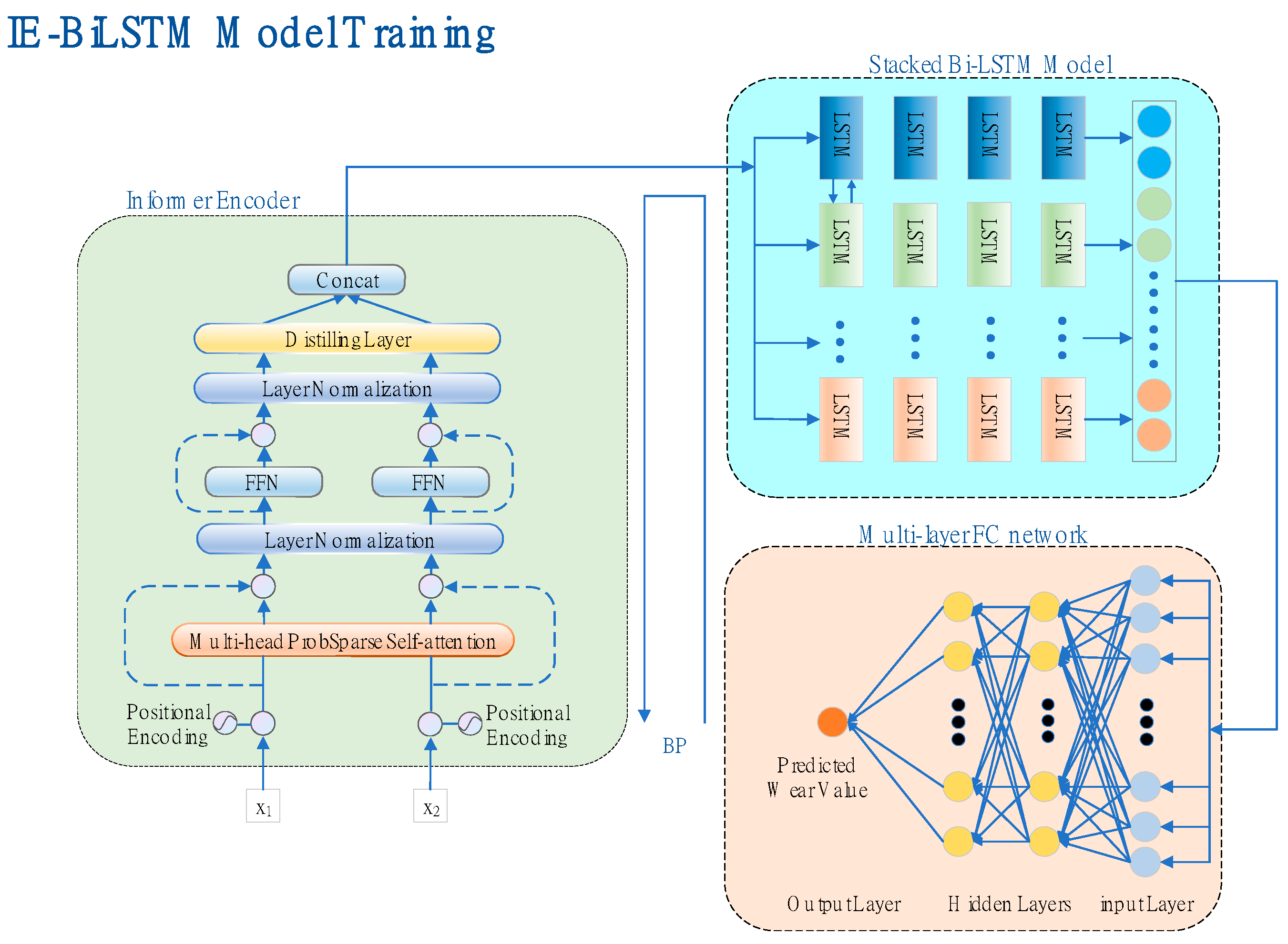
• This study proposed a new and effective tool-wear monitoring and evaluation method. This is the first time that a combination of an informer encoder and the Bi-LSTM model has been used for tool-wear monitoring. The experimental results show that this method is superior to other methods in terms of related evaluation indexes.
• The informer encoder was employed as the global feature extractor for multichannel long-term feature sequences, and computational efficiency was enhanced by employing sparse self-attention.
• The Bi-LSTM module was used to enhance the ability to capture the feature dependence of long-distance time series.

The remainder of this essay is structured as follows: The main idea behind the suggested model module is introduced in Section 2. The proposed method is explained in Section 3. The experimental findings are summarized in Section 4. The pertinent conclusions are summarized in Section 5.

2. Model Theory

To gather pertinent signals for this study, cutting force, vibration, and acoustic emission sensors are used. Corresponding data-driven models are created to ascertain how these signals relate to tool wear. Thus, the IE-Bi-LSTM model is proposed, comprising the informer encoder and Bi-LSTM modules. The following sections introduce the details of the two modules.

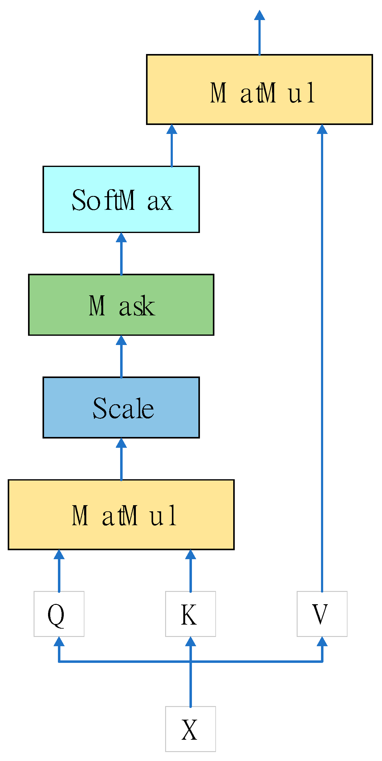
2.1. Scaled Dot-Product Attention

Figure 1 depicts the scaled dot-product attention structure. Scaled dot-product attention is the main element of the transformer model proposed by Vaswani et al. [30].

The scaled dot-product attention can be expressed as follows:

$$Attention(Q,K,V)=\mathrm{softmax}\left(\frac{Q{K}^T}{\sqrt{d_k}}\right)V$$

(1)

Assuming that the input node is x, the input will be mapped to a f(x) of the input embedding before being transformed to the corresponding Q, K, and V values through the transformation matrices $w_q$, $w_k$, and $w_v$, respectively, where Q, K, and V denote the query, key, and values, respectively, and $d$ denotes the length of vector K. Finally, the weight of the corresponding attention can be obtained using Equation (1). However, when the length of the input sequence increases, the double-dot-product operation, which is the primary flaw in its capacity for prediction, causes the computational overhead to increase significantly. This is the primary drawback of its ability to anticipate. Scaled dot-product attention has a long tail distribution at its output, meaning that only a small subset of dot products warrants any real consideration.

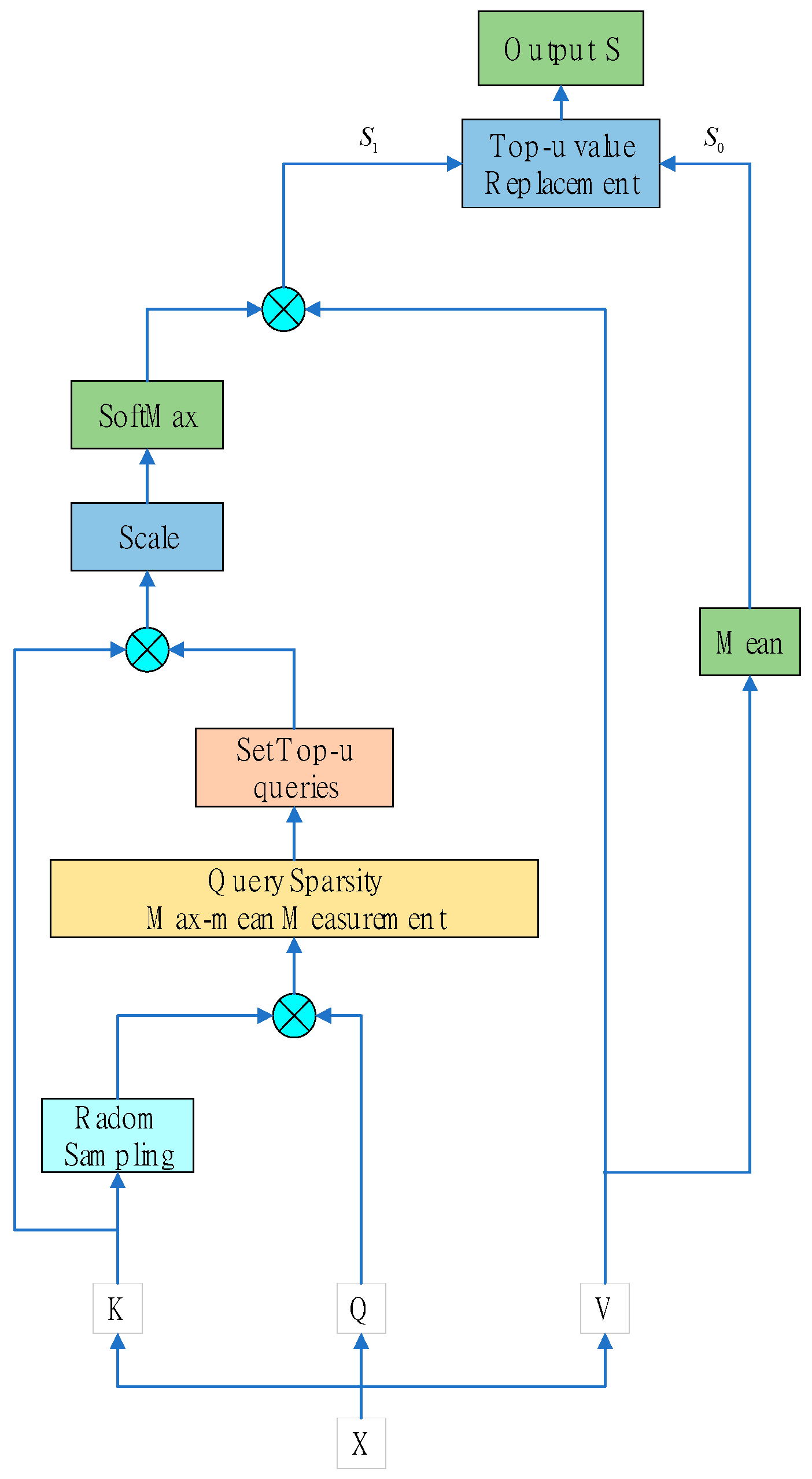
2.2. Prob-Sparse Self-Attention

To solve the self-attention problem, Zhou et al. [32] proposed using a probabilistic self-attention method, the structure of which is shown in Figure 2.

According to Zhou et al., scaled dot-product attention has a long tail distribution at its output, meaning that only a small subset of dot products warrants any real consideration. The dissimilarity between the two distributions can be evaluated with the help of Kullback–Leibler divergence [33], and the main dot-product pairs can be screened out, with the evaluation of the ith query sparsity being obtained as follows:

$$M\left(q_i,K\right)=\ln {\displaystyle \sum _{j=1}^{L_k}{e}^{\frac{q_i{k}_j^T}{\sqrt{d}}}}-\frac{1}{L_K}{\displaystyle \sum _{j=1}^{L_K}\frac{q_i{k}_j^T}{\sqrt{d}}}$$

(2)

The first term denotes the log-sum-exp of $q_i$ on all keys, with the second term being their arithmetic mean. To avoid memory bottlenecks caused by traversing all key-value pairs and potential numerical stability problems in the LSE operations, an empirical approximation of the maximum mean measurement based on Equation (3) is proposed:

$$\overline{M}\left(q_i,K\right)={\max }_j\left\{\frac{q_i{k}_j^{\top }}{\sqrt{d}}\right\}-\frac{1}{L_K}{\displaystyle \sum _{j=1}^{L_K}\frac{q_i{k}_j^{\top }}{\sqrt{d}}}$$

(3)

Prob-sparse self-attention can be used for dot-product calculation by randomly sampling $\log L$ points instead of selecting the entire L for calculation. The sparsity score $M\left(q_i,K\right)$ of each query can then be calculated, with u queries being selected from among all the sparsity scores. Thus, to determine the outcomes of the attention mechanism, we only need to compute the dot-product results of the top u query-key pairs. We directly replace the remaining query-key pairs with the mean $\overline{M}\left(q_i,K\right)$ of the input of the self-attention layer. This ensures that each prob-sparse self-attention layer has an input and an output sequence length of L, with the calculation method of u being expressed as follows:

$$u=c\times \ln L$$

(4)

where c denotes a constant sampling factor.

Based on the maximum mean measurement, probabilistic self-attention can be achieved by allowing only u major query vectors to be focused on per key, which is expressed as follows:

$$Proattention(Q,K,V)=\mathrm{Softmax}\left(\frac{\overline{\mathrm{Q}}{\mathrm{K}}^{\top }}{\sqrt{d}}\right)V$$

(5)

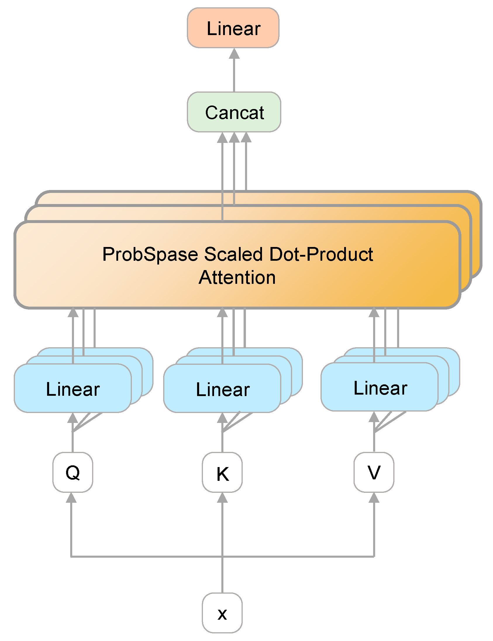
2.3. Informer Encoder

The structure of the informer encoder is shown in Figure 3, comprising a prob-sparse self-attention module and a distilling module. Among them, the prob-sparse self-attention module includes the multi-head sparse attention mechanism module, the residual connection, the position feedforward network component (FFN), and layer normalization (LN) [34], which are followed by each module. The convolution and maximum pooling layers make up the distillation module. The sections that follow provide descriptions of the primary modules.

2.3.1. Multi-Head Attention

The multi-head attention mechanism is introduced to improve the attention layer’s performance in two areas. To begin, it broadens the model’s capability of concentrating on a variety of regions. Second, it provides multiple “presentation subspaces” for the attention layer. The model can learn information in various presentation subspaces. Figure 4 depicts the multi-head self-attention module’s construction.

A linear transformation is initially applied to Q, K, and V in the linear layer. The self-attention layer is then fed the outcome of the linear transformation. The output values are connected in series, and then a linear transformation is applied to determine the final result. The results can be obtained using Equations (6) and (7) as follows:

$$\mathrm{MultiHead}(Q,K,V)=\mathrm{Concat}\left({\mathrm{head}}_1,\dots ,{\mathrm{head}}_{\mathrm{h}}\right)W^O$$

(6)

$$\mathrm{where}{\mathrm{head}}_{\mathrm{i}}=\mathrm{Attention}\left(Q{W}_i^Q,K{W}_i^K,V{W}_i^V\right),$$

(7)

where $W_i^Q\in {ℝ}^{d_{\mathrm{model}}\times d_k}$, $W_i^K\in {ℝ}^{d_{\mathrm{model}}\times d_k}$, and $W_i^V\in {ℝ}^{d_{\mathrm{model}}\times d_v}$ denote the parameter matrices, and $W^O\in {ℝ}^{h{d}_v\times d_{\mathrm{model}}}$ denotes the weight matrix. $d_k$ and $d_v$ represent the size of the Key and Value matrices, respectively. $d_k=d_v=d_{\mathrm{model}}/h$.

2.3.2. Position-Wise Feedforward Networks

Position-wise feedforward networks (FFNs) are fully connected feedforward networks in which the output of each model passes through the same feedforward neural network separately. It comprises two linear transformations—that is, two fully connected layers. The GELU activation function is the activation function of the first fully linked layer [35], which can be shown as follows:

$$\mathrm{FFN}\left(R_1\right)=\mathrm{Conv}1d\left(\mathrm{GELU}\left(\mathrm{Conv}1d\left(R\right)\right)\right)$$

(8)

where GELU denotes a nonlinear activation function, and $R$ indicates the result of the prior module [36].

2.3.3. Residual Connections and Layer Normalization

In the informer encoder, each sublayer of each encoder—that is, the self-attention and FFN layers—has a residual join, followed by a layer standardization operation, as shown in Figure 3. The addition of residual connections preserves the original information and prevents gradient disappearance. The normalization term scales the summed input when the LN is introduced, increasing the stability of the model during training and inference [37]. It also performs a normalizing role, which aids in accelerating the training process and accelerating convergence. The issues with vanishing and exploding gradients are also avoided by using LN layers. The calculation of $R_2$ can be expressed as follows:

$$R_2=\mathrm{LayerNorm}\left(R_1+\mathrm{FFN}\left(R_1\right)\right)$$

(9)

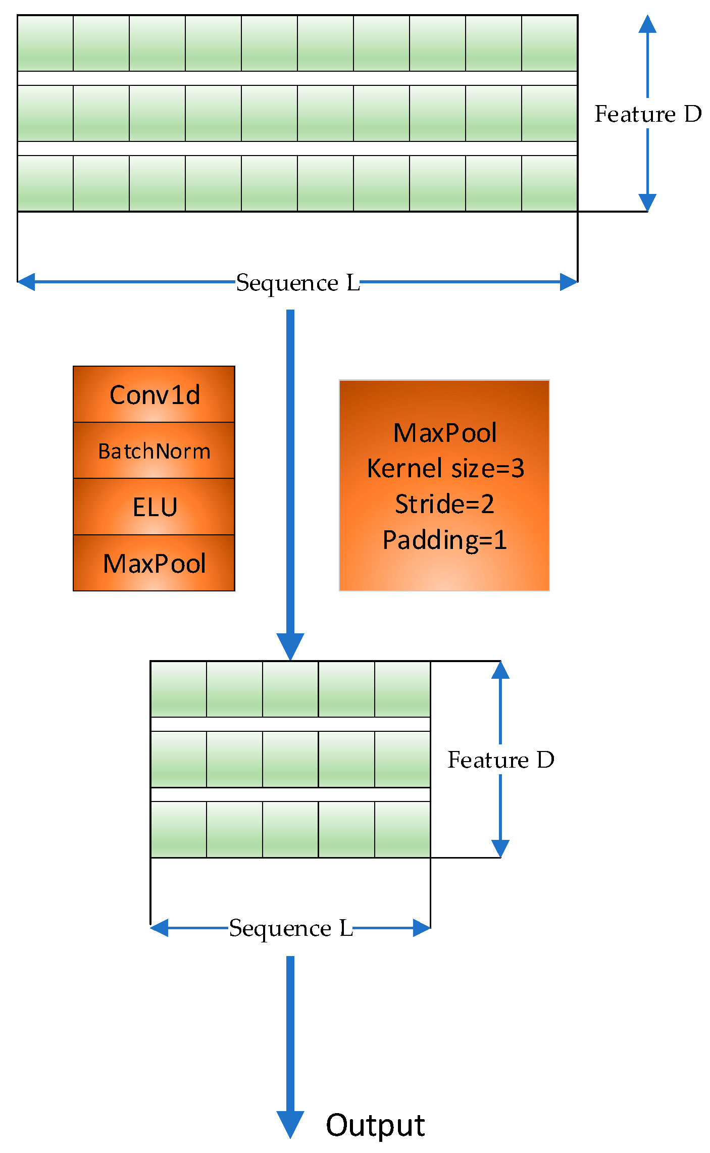
2.4. Distilling Layer

When the input sequence is too long, only the top u queries are selected in the above probability attention for dot-product operation to form Q-K pairs, whereas other Q-K pairs are set to average values. To solve the problem of information redundancy, a distillation layer is introduced at the end of the encoder, as shown in Figure 5. The introduction of a distillation layer highlights the main features, reduces the spatial complexity of long-sequence inputs, avoids the loss of information, and improves efficiency.

This module consists of the Conv1d, batch normalization, ELU activation, and the maximum pooling (MaxPool) operations. The “distillation” from the jth layer to the (j + 1)th layer can be expressed as follows:

$$X_{j+1}^t=\mathrm{MaxPool}\left(ELU\left(\mathrm{Conv}1d{\left[X_j^t\right]}_{AB}\right)\right)$$

(10)

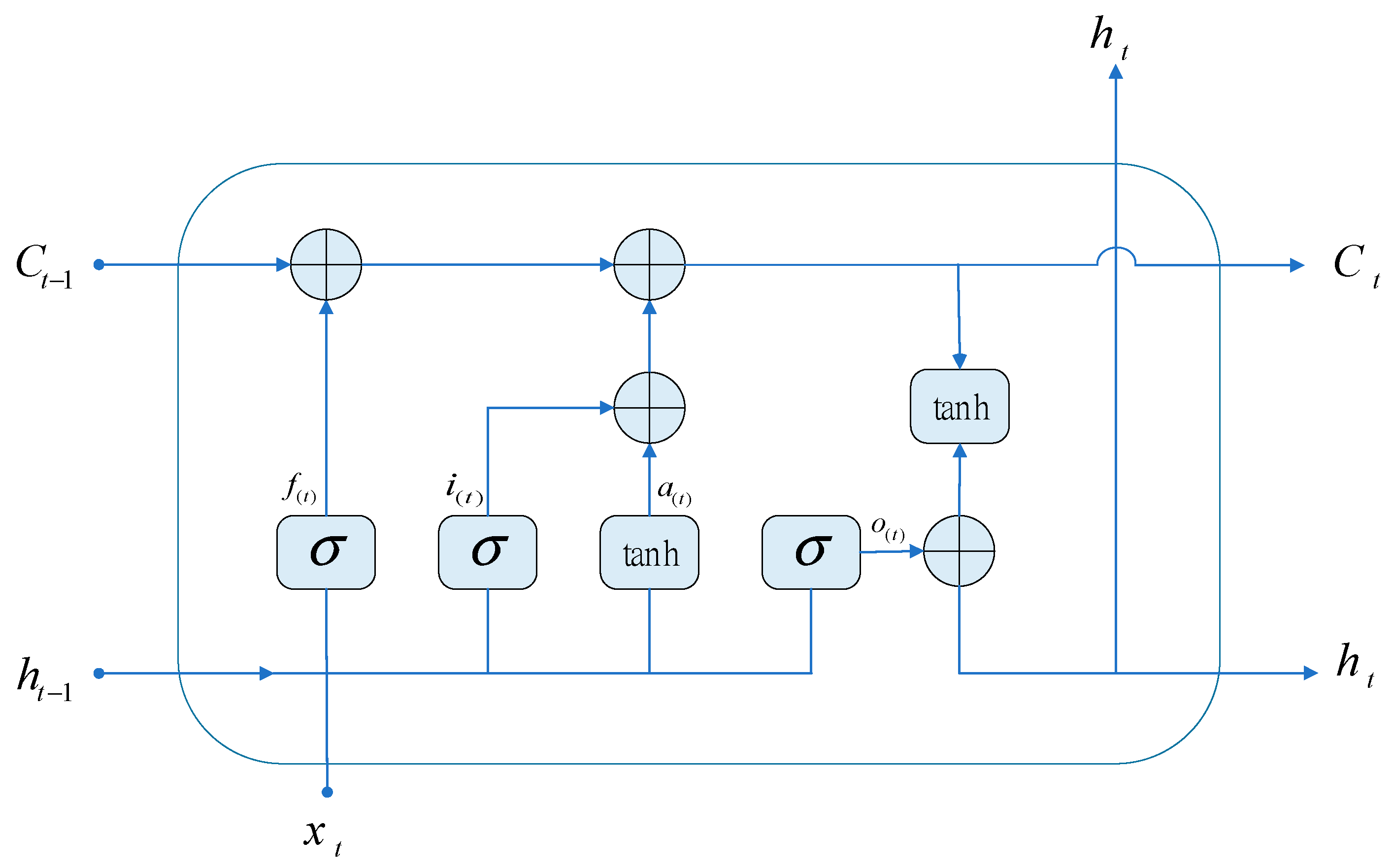
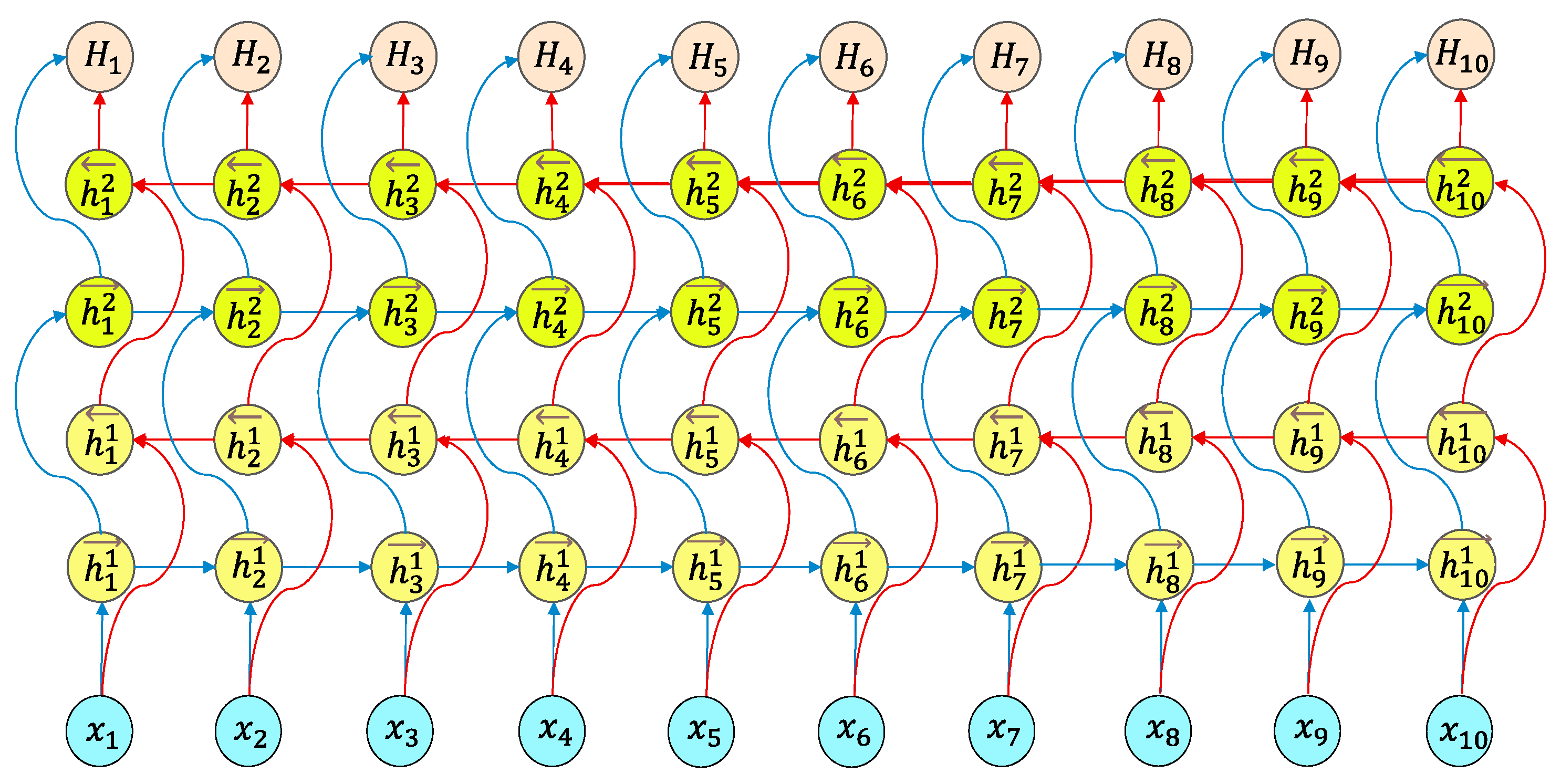
2.5. Bi-Directional Long Short-Term Memory

The problem of gradient vanishing occurs while the RNN is in the process of back propagation. This problem can cause the RNN to forget what it has learned in a long sequence, which can cause the RNN to malfunction. However, the primary structure of an LSTM is very similar to that of an RNN. The main difference is that an additional cell state and three gate structures are added to the hidden layer. These gate structures are known as the forget gate, the input gate, and the output gate. Figure 6 provides an illustration of the fundamental idea behind the LSTM hidden layer construction.

Through the forget control gate, the inputs $h_{t-1}$ and $x_t$ are read, and then $f(t)$ is obtained using the signal function layer. The inputs $h_{t-1}$ and $x_t$ travel through the signal function layer and the tanh function layer, respectively, in the input control gate to obtain $i(t)$ and $a_t$. In the output control gate, the inputs $h_{t-1}$ and $x_t$ obtain $o(t)$ through the signal function layer. Then, the precise mathematical procedure can be stated as follows:

$$f(t)=\sigma \left(W_f{h}_{t-1}+U_f{x}_t+b_f\right)$$

(11)

$$i(t)=\sigma \left(W_i{h}_{t-1}+U_i{x}_t+b_i\right)$$

(12)

$$a(t)=\tanh \left(W_a{h}_{t-1}+U_a{x}_t+b_a\right)$$

(13)

$$o(t)=\sigma \left(W_o{h}_{t-1}+U_o{x}_t+b_o\right)$$

(14)

$$\tanh (x)=\frac{1-e^{-2x}}{1+e^{-2x}}$$

(15)

$$\sigma (x)=\frac{1}{1+e^{-x}}$$

(16)

$W_f$, $W_i$, $W_o$, and $W_a$ indicate the forgetting gate, input gate, and output gate weight coefficients. $U_f$, $U_i$, $U_o$, and $U_a$ are used to express the weight coefficients of the forgetting gate, input gate, output gate, and feature extraction method, respectively. $b_f$, $b_i$, $b_o$, and $b_a$ represent the offset values of the forgetting gate, input gate, and output gate in the feature extraction process.

We acquire the final output $c(t)$ using $c(t-1)\times f(t)$, which indicates the discarding of the rejected information that we confirmed in the old information, and $i(t)\times a(t)$, which indicates the information that needs to be updated. The particular computation procedure can be stated as follows:

$$c(t)=c(t-1)\times f(t)+i(t)\times a(t)$$

(17)

The output gate $o(t)$ at the present time can be used to determine the hidden layer state $h(t)$ at time t as follows:

$$h(t)=o(t)\times \tanh (c(t))$$

(18)

The structural architecture of the Bi-LSTM neural network can be separated into two independent LSTM networks. The input sequences are processed by the two LSTM networks to extract features, one in the forwards direction and one in the backwards direction. The final feature expression of the word can be the word vector created by splicing the two output vectors. Figure 7 depicts the construction of the Bi-LSTM model.

The Bi-LSTM model’s goal is to make it possible for the feature data collected at time t to include information about both the past and the future. Previous experiments have shown that the efficiency and performance of this neural network structure for text feature extraction are better than those of a model with a single LSTM structure.

3. Methods: The IE-Bi-LSTM Model

The model proposed in this paper comprises data preprocessing, the IE-Bi-LSTM model, and a fully connected output layer. Based on the characteristics of the model given in this study, it is critical to examine the influence of historical information on tool wear. As a result, the entire initial signal is segmented using the sliding window function and then divided into training, verification, and test datasets. Three temporal features—the maximum, average, and variance values—for each channel are collected from each segment.

Figure 8 depicts the network structure and training procedure. The IE-Bi-LSTM model includes an informer encoder, the Bi-LSTM module, and a transport layer. After data preprocessing, a two-dimensional tensor is produced, which is utilized as the model’s input. The model, which is embedded with position coding, is then input into an informer encoder to extract the long time-series features. The extracted long series features can then be input into the Bi-LSTM module to enhance the long-distance time feature information, after which regression is carried out using the full connection layer. During training, the model weights and biases are updated using back propagation, with the mean square error serving as the loss function.

4. Experimental Results

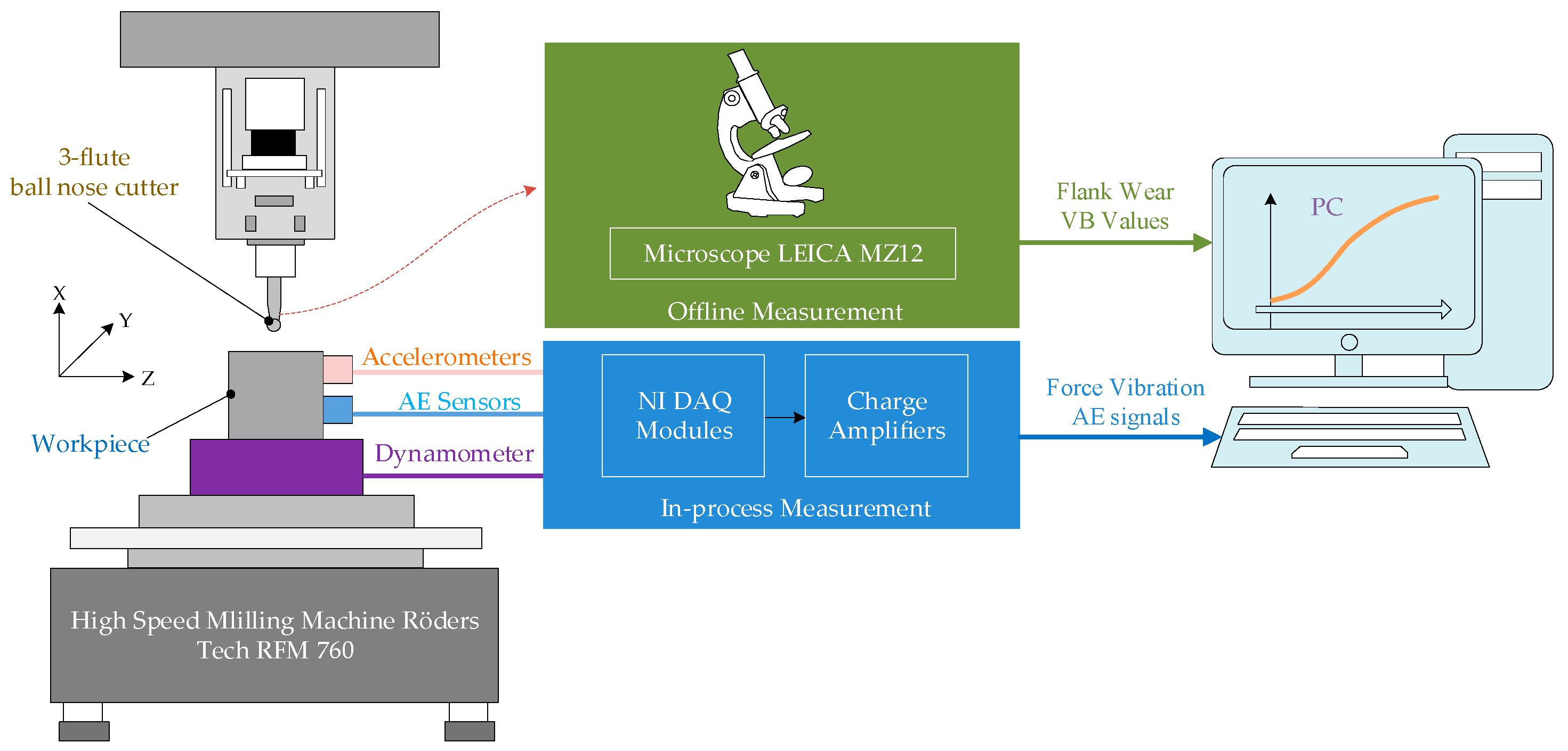
4.1. Dataset Descriptions

To verify the validity of the IE-Bi-LSTM model, the PHM2010 dataset [38] was used for model training and validation. The PHM2010 tool-wear dataset is available in the Data Availability Statement at the end of this article. The experimental system structure is shown in Figure 9. During the experiment, a Kistler quartz three-component platform dynamometer, a Kistler Piezoelectric acceleration sensor, and a Kistler AE sensor were used to collect X, Y, Z three-axis cutting force, three-axis vibration signal, and acoustic emission signal, respectively. The experiment used 6 mm three-flute ball carbide milling cutters for dry milling along the horizontal direction. The main equipment and process parameters are shown in

Table 1. Main equipment of the experimental setup.

Equipment	Type
CNC milling machine	Roders Tech RFM760
Dynamometer	Kistler 9265B
Charge amplifier	Kistler 5019A
Acoustic emission sensor	Kistler AE sensor
Cutters	3-flute ball carbide milling cutters
Data acquisition card	DAQ NI PCI 1200
Abrasion measuring apparatus	LEICA MZ12 microscope

and

Table 2. Experimental processing parameters.

Parameter	Value
Spindle	10,400/(r/min)
Feed rate	1555 (mm/min)
Depth of cut (y direction, radial)	0.125 (mm)
Depth of cut (z direction, axial)	0.2 (mm)
Sampling rate	50 (KHz)
Workpiece material	Stainless steel (HRC52)

. In the experiment, three milling cutters (C1, C4, and C6) of the same material were used under the same experimental conditions. Each milling cutter was subjected to 315 experiments under the same working conditions, each milling experiment took about 4 s, and the signals collected by each sensor were recorded in datasets. Therefore, about 200,000 measurement signals could be obtained per milling experiment per tool. Finally, the three cutters, C1, C4, and C6, were measured using a microscope after each milling, and the wear amount corresponding to each blade of the milling cutter was flute1-3. The wear measurement accuracy was 10⁻³ mm.

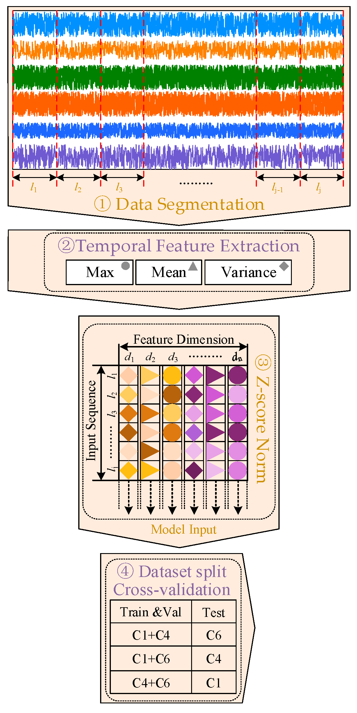
4.2. Data Preprocessing

When attempting to improve the model’s generalization capabilities, the deep learning process might result in a complicated network topology, resulting in a high number of model hyperparameters that must be trained. Consequently, the training dataset must have a large sample size. When the sample size is small, the deep learning network is prone to overfitting. Therefore, to ensure satisfactory training, it was necessary to enhance the original data of the collected data samples. Here, we introduced the average sampling enhancement method (ASA) [39], which enhanced the target signal samples by evenly collecting the signal segment of the target length through a sliding window in the target signal. After signal preprocessing, each new sample was used as an input to the deep learning model.

Because of the damage to the cutting force signal in the x-direction, data from the other six channels were used in this experiment. As shown in Figure 10, the data preprocessing operations were performed sequentially. First, the entire sequence was decomposed using the sliding window method along the direction of the time dimension. The maximum, average, and variance values were then extracted from each channel and connected to form the feature data sample. The size of the feature data sample was ${ℝ}^{120\times 18}$. The model input $x_i$ was then obtained through normalization along the direction of the time series, with the model converging quickly through the normalization operation. The wear label was chosen based on the maximum value of the three wear surfaces for safety concerns. After data preprocessing, the C1 dataset included 57,529 sets of data, the C4 dataset included 58,449 sets of data, and the C6 dataset included 57,485 sets of data. Finally, cross-validation was used to select two datasets as the training and verification datasets, with the remaining dataset being the test set. The ratio of the training dataset to the validation dataset was 4:1.

4.3. Experimental Environment and Hyperparameter Configuration

Personal desktops, with Intel Core i9 11900k CPU, 128 GB of memory, NVIDIA RTX 3090 GPU, and 24 GB of video memory, were used for the experimental platform. For this study, we built a Pytorch deep learning framework on a Windows 10 operating system. Python was used to create the program code and call the necessary libraries, including CUDA and CUDNN, using the software environments CUDA 10.1, CUDNN 7.6, and Python3.8. In this way, we effectively trained and tested the firefighting robot flame recognition model.

The deep learning network model effect might be positive or negative, depending on the hyperparameters used. The batch size, dropout rate, and learning rate were the primary hyperparameters in the IE-Bi-LSTM model. The number of heads in the multi-head self-attention mechanism was another important hyperparameter (H). These hyperparameters were changed based on the model’s performance on the verification dataset, with the hyperparameter with the lowest loss value chosen as the default parameter. The Adam optimizer was used during the model training [22]. L2 regularization and discarding, among other techniques, were used to prevent overfitting during model training.

Table 3. Hyperparameter settings.

Parameters	Learning Rate	Epoch	Batch Size	Dropout
Values	0.001	100	32	0.2
Parameters	Warmup	FC neurons	H	Activation
Values	20	64/64/1	3	ReLu

lists the specific hyperparameter settings.

4.4. Experimental Environment and Hyperparameter Configuration

The IE-Bi-LSTM model’s evaluation indices used in this work were the mean absolute error (MAE) and the root mean square error (RMSE), whose formulas are as follows:

$$MAE=\frac{1}{n}{\displaystyle \sum _{i=1}^n\left|y_i-f_i\right|}$$

(19)

$$RMSE=\sqrt{\frac{1}{n}{\displaystyle \sum _{i=1}^n{\left(y_i-f_i\right)}^2}},$$

(20)

where $y_i$ denotes the ith predicted value, and $f_i$ denotes the ith true value. The smaller the MAE and RMSE values, the more effective these evaluation indices are in tool-wear prediction applications. Consequently, we compared these evaluation indices with other published results.

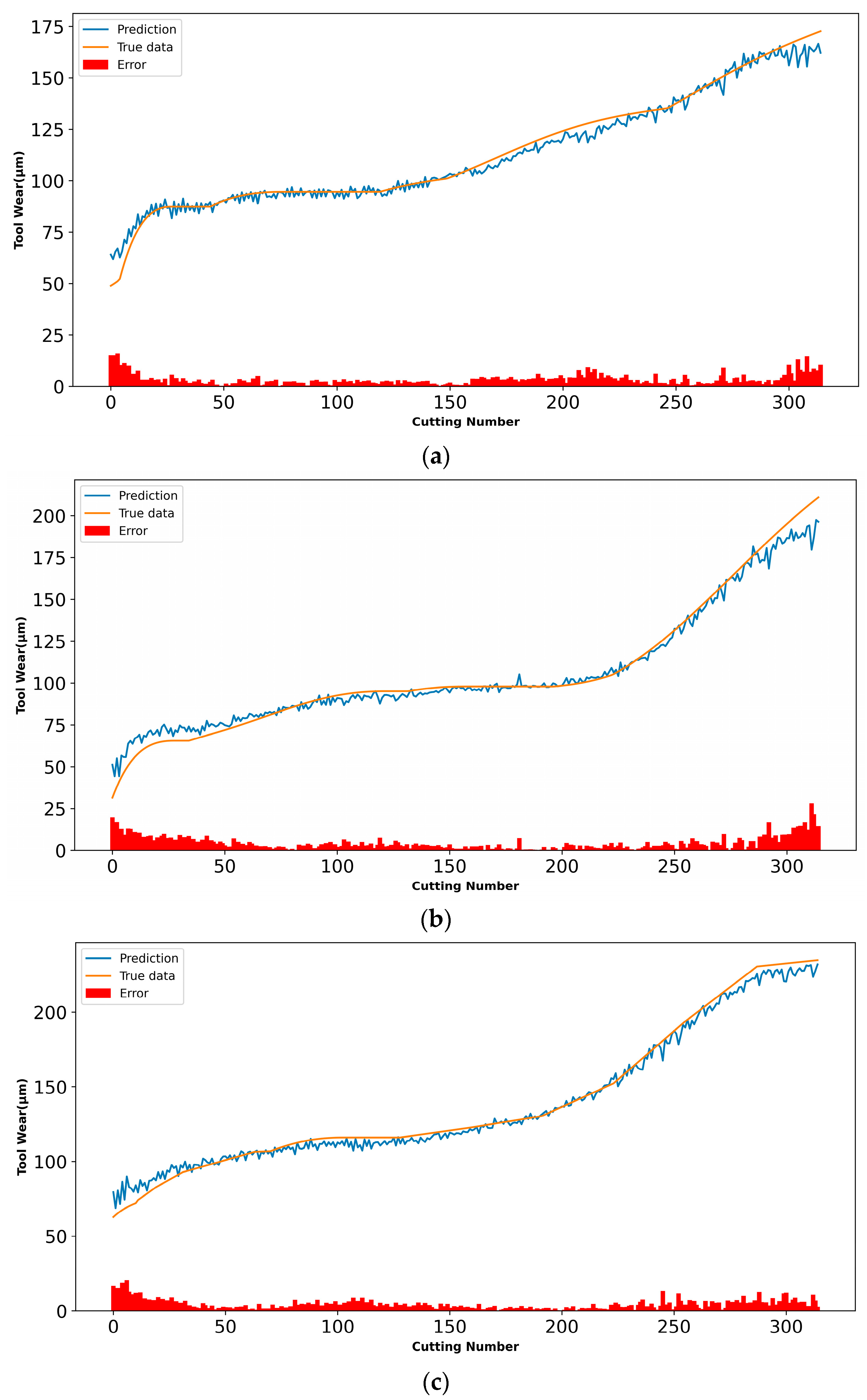
4.5. Experimental Results and Analysis

In order to make the experiment more objective, each experiment was carried out 10 times under the same conditions, and the average value of the 10 experimental results was taken as the final result. The IE-Bi-LSTM model obtained good results in terms of the corresponding evaluation indicators.

The associated experimental findings are shown in Figure 11, together with the projected and actual tool-wear values, as well as the difference between the two. The projected tool surface wear curve is essentially compatible with the actual tool surface wear curve, and the majority of the errors are contained within a narrow range, which supports the model’s validity.

It can be seen in Figure 11 that the wear amount of the tool increases rapidly at the initial stage, and then the wear rate slows down. This is because the tool wear process can be divided into three stages, namely, the initial wear stage, the normal wear stage, and the sharp wear stage. In the initial wear stage of the tool, the newly sharpened tool has just been put into use, the actual contact area between the flank and the workpiece is small, the positive pressure per unit area is relatively large, and the surface roughness of the tool is rough or the surface structure of the tool is not wear-resistant, so the wear is faster in a short time when cutting starts. In the normal wear stage of the tool, after the initial wear, the contact area between the tool flank and the workpiece increases, the pressure on the unit area gradually decreases, and the microscopic rough surface of the tool flank is ground, so the wear speed slows down.

It can also be seen in Figure 11 that, in the initial stage, the error between the predicted value and the real value is large. This is because, in the early stage, the tool wear amount is small, and the IE-Bi-LSTM model learns fewer features. As the amount of wear increases, more features are learned by the IE-Bi-LSTM model, so the error between the predicted value and the real value decreases. In the final stage of increased tool wear, the error between the predicted value and the real value increases, because the signal collected by the sensor includes more noise, which affects the accuracy of the IE-Bi-LSTM model prediction.

This study compared the results of the IE-Bi-LSTM model with those of several classical methods and contemporary methods using the same dataset to further demonstrate the model’s usefulness and superiority. The MAE and RMSE values for the three tools used with these models are listed in

Table 4. Performance comparisons with other models.

Models	Datasets
	C1		C4		C6
	MAE	RMSE	MAE	RMSE	MAE	RMSE
RNN [21]	13.1	15.6	16.7	20	25.5	32.91
Bi-LSTM [40]	12.8	14.6	10.9	14.2	14.7	17.7
CNN-LSTM [41]	11.18	13.77	9.39	11.85	11.34	14.33
Deep-LSTM [21]	8.3	12.1	8.7	10.2	15.2	18.9
HLLSTM [40]	6.6	8	6	7.5	7.1	8.8
TBNN [31]	4.294	6.116	/	/	7.772	9.553
CTNN [42]	3.634	5.358	/	/	7.531	9.209
LF-GRU [43]	4.2	5.4	6.9	8.3	5.8	8.2
DH-GRU [44]	3.7	4.66	7.07	8.73	5.08	6.94
IE-SBIGRU [36]	3.694	5.056	5.189	6.884	3.398	4.527
Proposed model	2.68	3.23	3.09	3.91	3.37	4.27

.

As is evident in Table 4, the proposed model achieves optimal results in comparison with the other models, indicating that the IE-Bi-LSTM model performs well on the PHM2010 dataset, proving the effectiveness of the model.

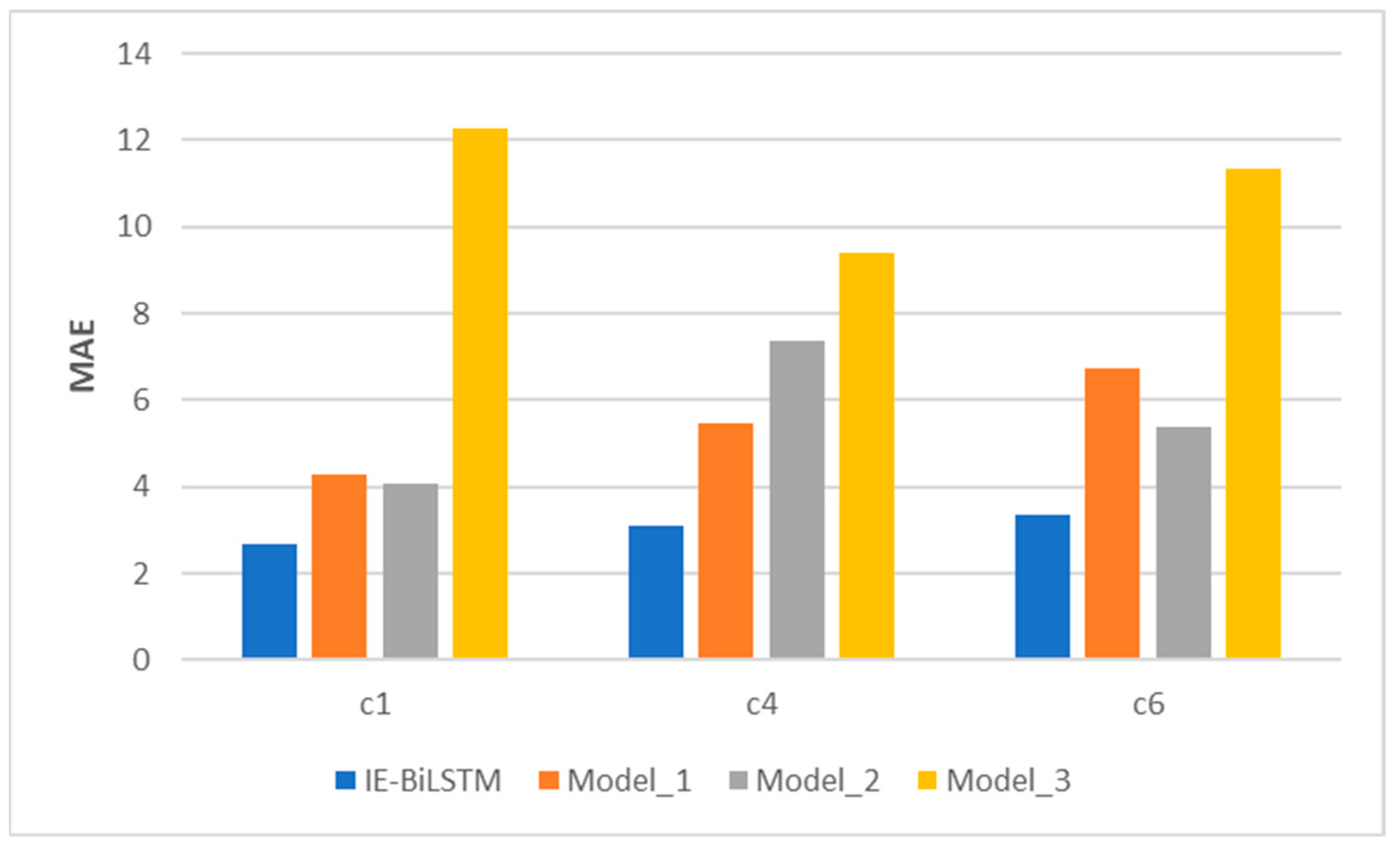
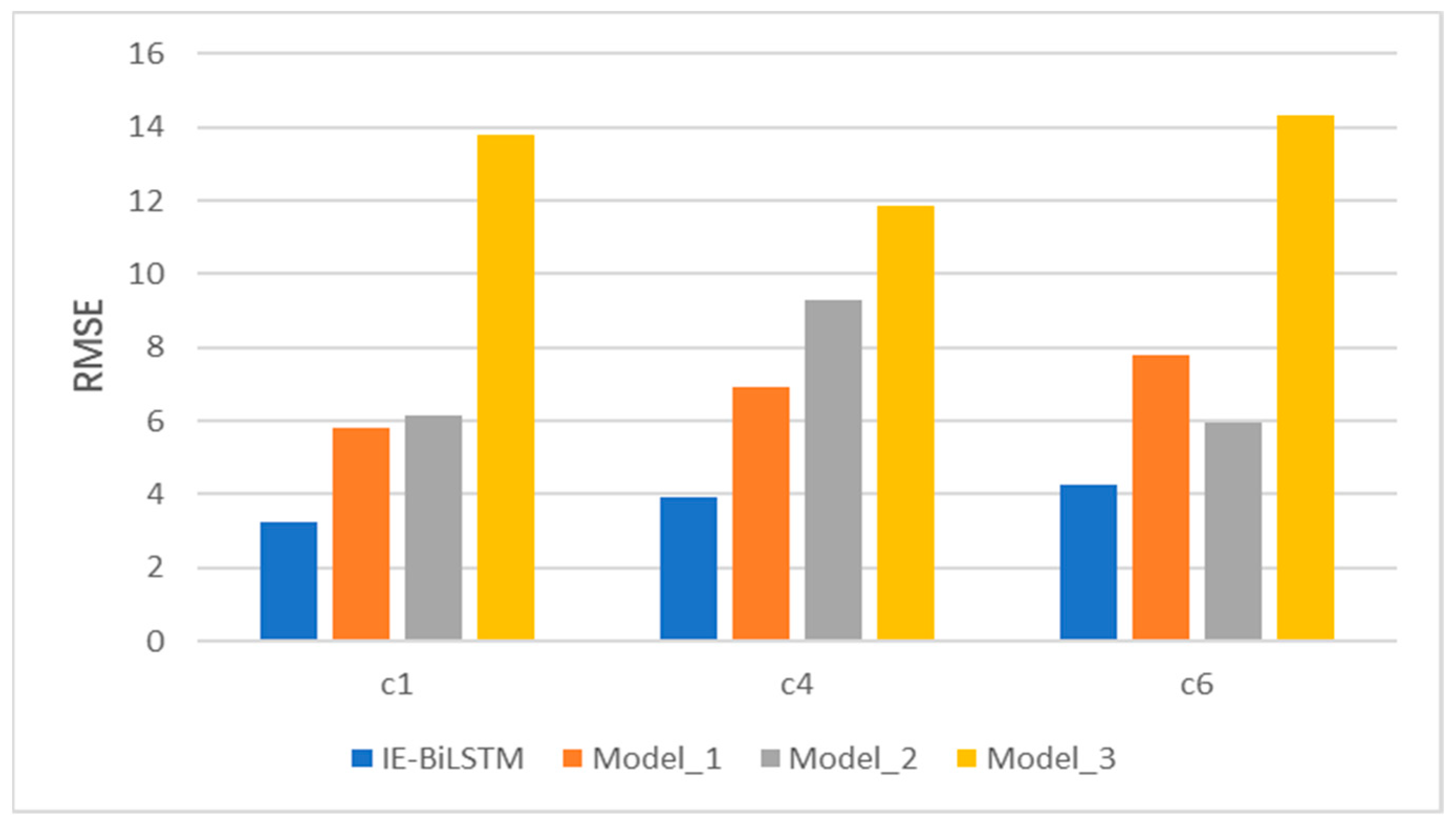
4.6. Model Module Analysis

Because the IE-Bi-LSTM model improved based on its integration of the informer model, to understand the performance of the modules in the IE-Bi-LSTM model, a comparative test was conducted. We designed three models with an architecture similar to that of the proposed model, all of which had similar hyperparameters. Scaled dot-product attention was utilized in Model 1 in place of prob-sparse self-attention, and the distillation layer was eliminated in Model 2. As a result of Model 2, the encoder had a fixed sequence length. The Bi-LSTM layer was deleted in Model 3. The comparison results are shown in Figure 12.

In terms of the key performance measures, the comparative results in Figure 12 reveal that the IE-Bi-LSTM model outperforms the other three models. Compared with Model 1, the IE-Bi-LSTM model with the integrated prob-sparse self-attention method achieves the best results in terms of the MAE and RMSE values. Because dot-product attention necessitates the calculation of all key-value pairs, the model’s computational cost rises. Similarly, in the actual tool-wear application scenario, this calculation method can lead to the retention of a large volume of redundant information. These factors make the model ineffective for extracting tool-wear features. The addition of the distillation layer increases the model’s computational efficiency and prediction accuracy when compared to those of Model 2. Compared with Model 3, it is evident that the single-informer model cannot effectively predict tool wear, and its prediction ability is limited.

The introduction of the Bi-LSTM module effectively enhances the model’s ability to capture the position relationship between long-distance features and improves its prediction ability, proving the effectiveness of the improvements introduced in this study.

5. Conclusions and Future Work

To make more precise tool-wear predictions, a new model based on an informer model was developed in this work. The proposed model makes two major contributions to the literature. First, it combined the informer model with the Bi-LSTM model for the first time, making relevant improvements for specific tool-wear prediction scenarios. For example, prob-sparse self-attention was used to reduce the computational complexity of the model to $\mathrm{O}(\mathrm{LlogL})$, and it was introduced to enhance the position relationship between long-distance features. Furthermore, the efficacy of the suggested model was demonstrated in experiments using the PHM2010 dataset. Additionally, ablation experiments were conducted to study the effectiveness of each improved module in predicting tool wear.

Future research could examine how different spindle and feed mechanisms in CNC machine tools affect tool wear, combined with several factors of various other systems to further improve the predictive performance of tool wear. Moreover, we could further study the practical applications of a multitask method in tool-wear prediction.

References

1. Baroroh, D.K.; Chu, C.; Wang, L. Systematic literature review on augmented reality in smart manufacturing: Collaboration between human and computational intelligence. J. Manuf. Syst. 2021, 61, 696–711. [Google Scholar] [CrossRef]
2. Yu, H.; Wang, K.; Zhang, R.; Wu, X.; Tong, Y.; Wang, R.; He, D. An improved tool wear monitoring method using local image and fractal dimension of workpiece. Math. Probl. Eng. 2021, 2021, 9913581. [Google Scholar] [CrossRef]
3. Kurada, S.; Bradley, C. A review of machine vision sensors for tool condition monitoring. Comput. Ind. 1997, 34, 55–72. [Google Scholar] [CrossRef]
4. Li, Y.; Liu, C.; Hua, J.; Gao, J.; Maropoulos, P. A novel method for accurately monitoring and predicting tool wear under varying cutting conditions based on meta-learning. CIRP Ann. 2019, 68, 487–490. [Google Scholar] [CrossRef]
5. Duan, J.; Zhang, X.; Shi, T. A hybrid attention-based paralleled deep learning model for tool wear prediction. Expert Syst. Appl. 2023, 211, 118548. [Google Scholar] [CrossRef]
6. Lins, R.G.; de Araujo, P.R.M.; Corazzim, M. In-process machine vision monitoring of tool wear for Cyber-Physical Production Systems. Robot. Comput.-Integr. Manuf. 2020, 61, 101859. [Google Scholar] [CrossRef]
7. Wang, J.; Xie, J.; Zhao, R.; Zhang, L.; Duan, L. Multisensory fusion based virtual tool wear sensing for ubiquitous manufacturing. Robot. Comput.-Integr. Manuf. 2017, 45, 47–58. [Google Scholar] [CrossRef] [Green Version]
8. Zhang, C.; Zhang, H. Modelling and prediction of tool wear using LS-SVM in milling operation. Int. J. Comput. Integr. Manuf. 2016, 29, 76–91. [Google Scholar] [CrossRef]
9. Shi, D.; Gindy, N.N. Tool wear predictive model based on least squares support vector machines. Mech. Syst. Signal Process. 2007, 21, 1799–1814. [Google Scholar] [CrossRef]
10. Atlas, L.; Ostendorf, M.; Bernard, G.D. Hidden Markov models for monitoring machining tool-wear. In Proceedings of the 2000 IEEE International Conference on Acoustics, Speech, and Signal Processing, Istanbul, Turkey, 5–9 June 2000; (Cat. No. 00CH37100). pp. 3887–3890. [Google Scholar]
11. Zhu, K.; San Wong, Y.; Hong, G.S. Multi-category micro-milling tool wear monitoring with continuous hidden Markov models. Mech. Syst. Signal Process. 2009, 23, 547–560. [Google Scholar] [CrossRef]
12. Ertunc, H.M.; Loparo, K.A.; Ocak, H. Tool wear condition monitoring in drilling operations using hidden Markov models (HMMs). Int. J. Mach. Tools Manuf. 2001, 41, 1363–1384. [Google Scholar] [CrossRef]
13. Sick, B. On-line and indirect tool wear monitoring in turning with artificial neural networks: A review of more than a decade of research. Mech. Syst. Signal Process. 2002, 16, 487–546. [Google Scholar] [CrossRef]
14. Ezugwu, E.O.; Arthur, S.J.; Hines, E.L. Tool-wear prediction using artificial neural networks. J. Mater. Process. Technol. 1995, 49, 255–264. [Google Scholar] [CrossRef]
15. Zhang, C.; Wang, W.; Li, H. Tool wear prediction method based on symmetrized dot pattern and multi-covariance Gaussian process regression. Measurement 2022, 189, 110466. [Google Scholar] [CrossRef]
16. Liao, X.; Zhou, G.; Zhang, Z.; Lu, J.; Ma, J. Tool wear state recognition based on GWO–SVM with feature selection of genetic algorithm. Int. J. Adv. Manuf. Technol. 2019, 104, 1051–1063. [Google Scholar] [CrossRef]
17. Dong, J.; Subrahmanyam, K.; Wong, Y.S.; Hong, G.S.; Mohanty, A.R. Bayesian-inference-based neural networks for tool wear estimation. Int. J. Adv. Manuf. Technol. 2006, 30, 797–807. [Google Scholar] [CrossRef]
18. Wang, L.; Mehrabi, M.G.; Kannatey-Asibu, E., Jr. Hidden Markov model-based tool wear monitoring in turning. J. Manuf. Sci. Eng. 2002, 124, 651–658. [Google Scholar] [CrossRef]
19. Palanisamy, P.; Rajendran, I.; Shanmugasundaram, S. Prediction of tool wear using regression and ANN models in end-milling operation. Int. J. Adv. Manuf. Technol. 2008, 37, 29–41. [Google Scholar] [CrossRef]
20. Sun, H.; Zhang, J.; Mo, R.; Zhang, X. In-process tool condition forecasting based on a deep learning method. Robot. Comput.-Integr. Manuf. 2020, 64, 101924. [Google Scholar] [CrossRef]
21. Zhao, R.; Wang, J.; Yan, R.; Mao, K. Machine health monitoring with LSTM networks. In Proceedings of the 2016 10th International Conference on Sensing Technology (ICST), Nanjing, China, 11–13 November 2016; pp. 1–6. [Google Scholar]
22. Duan, J.; Duan, J.; Zhou, H.; Zhan, X.; Li, T.; Shi, T. Multi-frequency-band deep CNN model for tool wear prediction. Meas. Sci. Technol. 2021, 32, 65009. [Google Scholar] [CrossRef]
23. Sun, C.; Ma, M.; Zhao, Z.; Tian, S.; Yan, R.; Chen, X. Deep transfer learning based on sparse autoencoder for remaining useful life prediction of tool in manufacturing. IEEE Trans. Ind. Inform. 2018, 15, 2416–2425. [Google Scholar] [CrossRef]
24. Marani, M.; Zeinali, M.; Songmene, V.; Mechefske, C.K. Tool wear prediction in high-speed turning of a steel alloy using long short-term memory modelling. Measurement 2021, 177, 109329. [Google Scholar] [CrossRef]
25. Liu, X.; Zhang, B.; Li, X.; Liu, S.; Yue, C.; Liang, S.Y. An approach for tool wear prediction using customized DenseNet and GRU integrated model based on multi-sensor feature fusion. J. Intell. Manuf. 2022, 1–18. [Google Scholar] [CrossRef]
26. Cao, X.; Chen, B.; Yao, B.; He, W. Combining translation-invariant wavelet frames and convolutional neural network for intelligent tool wear state identification. Comput. Ind. 2019, 106, 71–84. [Google Scholar] [CrossRef]
27. Huang, Z.; Zhu, J.; Lei, J.; Li, X.; Tian, F. Tool wear predicting based on multi-domain feature fusion by deep convolutional neural network in milling operations. J. Intell. Manuf. 2020, 31, 953–966. [Google Scholar] [CrossRef]
28. Cheng, M.; Jiao, L.; Yan, P.; Jiang, H.; Wang, R.; Qiu, T.; Wang, X. Intelligent tool wear monitoring and multi-step prediction based on deep learning model. J. Manuf. Syst. 2022, 62, 286–300. [Google Scholar] [CrossRef]
29. Bazi, R.; Benkedjouh, T.; Habbouche, H.; Rechak, S.; Zerhouni, N. A hybrid CNN-BiLSTM approach-based variational mode decomposition for tool wear monitoring. Int. J. Adv. Manuf. Technol. 2022, 119, 3803–3817. [Google Scholar] [CrossRef]
30. Vaswani, A.; Shazeer, N.; Parmar, N.; Uszkoreit, J.; Jones, L.; Gomez, A.N.; Kaiser, A.; Polosukhin, I. Attention is all you need. Adv. Neural Inf. Process. Syst. 2017, 30, 5998–6008. [Google Scholar]
31. Liu, H.; Liu, Z.; Jia, W.; Lin, X.; Zhang, S. A novel transformer-based neural network model for tool wear estimation. Meas. Sci. Technol. 2020, 31, 65106. [Google Scholar] [CrossRef]
32. Zhou, H.; Zhang, S.; Peng, J.; Zhang, S.; Li, J.; Xiong, H.; Zhang, W. Informer: Beyond efficient transformer for long sequence time-series forecasting. Proc. AAAI Conf. Artif. Intell. 2021, 35, 11106–11115. [Google Scholar] [CrossRef]
33. Zong, C.; Nie, J.; Zhao, D.; Feng, Y. Natural language processing and Chinese computing. Commun. Comput. Inf. Sci. 2012, 333, 262–273. [Google Scholar]
34. Ba, J.L.; Kiros, J.R.; Hinton, G.E. Layer normalization. arXiv 2016, arXiv:1607.06450. [Google Scholar]
35. Hendrycks, D.; Gimpel, K. Gaussian error linear units (gelus). arXiv 2016, arXiv:1606.08415. [Google Scholar]
36. Li, W.; Fu, H.; Han, Z.; Zhang, X.; Jin, H. Intelligent tool wear prediction based on Informer encoder and stacked bidirectional gated recurrent unit. Robot. Comput.-Integr. Manuf. 2022, 77, 102368. [Google Scholar] [CrossRef]
37. Li, J.; Wang, T.; Zhang, W. An improved Chinese named entity recognition method with TB-LSTM-CRF. In Proceedings of the 2020 2nd Symposium on Signal Processing Systems, Guangzhou China, 11–13 July 2020; pp. 96–100. [Google Scholar]
38. PHM Society: 2010 PHM Society Conference Data Challenge. Available online: https://www.phmsociety.org/competition/phm/10 (accessed on 31 December 2022).
39. Wen, L.; Li, X.; Gao, L.; Zhang, Y. A new convolutional neural network-based data-driven fault diagnosis method. IEEE Trans. Ind. Electron. 2017, 65, 5990–5998. [Google Scholar] [CrossRef]
40. Chan, Y.; Kang, T.; Yang, C.; Chang, C.; Huang, S.; Tsai, Y. Tool wear prediction using convolutional bidirectional LSTM networks. J. Supercomput. 2022, 78, 810–832. [Google Scholar] [CrossRef]
41. Qiao, H.; Wang, T.; Wang, P.; Qiao, S.; Zhang, L. A time-distributed spatiotemporal feature learning method for machine health monitoring with multi-sensor time series. Sensors 2018, 18, 2932. [Google Scholar] [CrossRef] [Green Version]
42. Liu, H.; Liu, Z.; Jia, W.; Zhang, D.; Wang, Q.; Tan, J. Tool wear estimation using a CNN-transformer model with semi-supervised learning. Meas. Sci. Technol. 2021, 32, 125010. [Google Scholar] [CrossRef]
43. Zhao, R.; Wang, D.; Yan, R.; Mao, K.; Shen, F.; Wang, J. Machine health monitoring using local feature-based gated recurrent unit networks. IEEE Trans. Ind. Electron. 2017, 65, 1539–1548. [Google Scholar] [CrossRef]
44. Wang, J.; Yan, J.; Li, C.; Gao, R.X.; Zhao, R. Deep heterogeneous GRU model for predictive analytics in smart manufacturing: Application to tool wear prediction. Comput. Ind. 2019, 111, 1–14. [Google Scholar] [CrossRef]
Figure 1. The scaled dot-product attention architecture.
Machines 11 00094 g001
Figure 2. The prob-sparse self-attention architecture.
Machines 11 00094 g002
Figure 3. Illustration of the informer encoder.
Machines 11 00094 g003
Figure 4. Illustration of the multi-head attention layer.
Machines 11 00094 g004
Figure 5. Illustration of the distilling layer.
Machines 11 00094 g005
Figure 6. Graphical illustration of the LSTM.
Machines 11 00094 g006
Figure 7. Graphical illustration of the Bi-LSTM layers used in the IE-Bi-LSTM model.
Machines 11 00094 g007
Figure 8. Illustration of the proposed method.
Machines 11 00094 g008
Figure 9. Illustration of the experimental setup.
Machines 11 00094 g009
Figure 10. Data preprocessing program.
Machines 11 00094 g010
Figure 11. Comparisons between the predicted tool wear and the ground-truth tool wear: (a) C1 cutter, (b) C4 cutter, and (c) C6 cutter.
Machines 11 00094 g011
Figure 12. Estimation performance of different models using the PHM2010 testing dataset.
Machines 11 00094 g012aMachines 11 00094 g012b