Line-Structured Light Fillet Weld Positioning Method to Overcome Weld Instability Due to High Specular Reflection

Abstract

Fillet welds of highly reflective materials are common in industrial production. It is a great challenge to accurately locate the fillet welds of highly reflective materials. Therefore, this paper proposes a fillet weld identification and location method that can overcome the negative effects of high reflectivity. The proposed method is based on improving the semantic segmentation performance of the DeeplabV3+ network for structural light and reflective noise, and, with MobilnetV2, replaces the main trunk network to improve the detection efficiency of the model. To solve the problem of the irregular and discontinuous shapes of the structural light skeleton extracted by traditional methods, an improved closing operation using dilation in a combined Zhang-suen algorithm was proposed for structural light skeleton extraction. Then, a three-dimensional reconstruction as a mathematical model of the system was established to obtain the coordinates of the weld feature points and the welding-torch angle. Finally, many experiments on highly reflective stainless steel fillet welds were carried out. The experimental results show that the average detection errors of the system in the Y-axis and Z-axis are 0.3347 mm and 0.3135 mm, respectively, and the average detection error of the welding torch angle is 0.1836° in the test of a stainless steel irregular fillet weld. The method is robust, universal, and accurate for highly reflective irregular fillet welds.

1. Introduction

Welding automation is applied in many manufacturing fields [1,2,3,4], among which one of the most complex applications is in robot-based autonomous welding systems [5,6,7], which use visual detection [8,9,10] to realize weld positioning and guidance, which is an important way to achieve intelligent robotic welding. By means of visual sensing, information in the human environment is processed and converted into position data that can be recognized by the controller and is then sent to the executing equipment for positioning and welding. With the improvement of welding production requirements, structured light vision welding seam-tracking technology is also facing new challenges. There are a large number of fillet welds needed in hull welding and new energy battery-box welding production. The hulls are made of stainless steel and the battery boxes are made from aluminum alloy, all of which are highly reflective materials. To identify and locate such fillet welds, it is necessary to overcome the interference in visual imaging when working on materials with high specular reflection. At present, there are few studies available on the visual positioning of highly reflective fillet welds, and there are few application products that can meet the actual production demand. Against this background, it is of great practical significance to study the positioning method of stainless-steel right-angle welds and develop related system software solutions.

The detection and positioning of welds using the machine vision method can be divided into active [11,12,13] and passive [14,15,16,17] detection, according to the different light source systems. In passive visual detection, monocular or binocular cameras directly capture images of the welding parts and extract the weld’s feature information via image processing, to then visualize the weld positioning.

Technology based on passive vision includes robot arc-welding fillet detection, based on an adaptive line growth algorithm proposed by Mitchell [18]. In this paper, an adaptive line-growth algorithm based on initial seed positions is introduced that can automatically identify fillet welds. Active vision is employed to project structural light onto the welding parts and reflect the structural features of the welding parts, according to the imaging features of structural light. Compared to passive vision, active vision is more stable and versatile. Du et al. [19] studied several weld-image algorithms to combat strong noise in robot GMAW, and adopted fast image segmentation, feature region recognition, and feature search technology in a convolutional neural network (CNN) to accurately identify the weld features. Yu et al. [20] proposed a method of structural light strip centerline weld extraction, based on a pyramid scene analysis network and a Steger algorithm. The ability to recognize the centerline of structural light under the influence of reflection interference is optimized. Zhao et al. [21], guided by the overexposure characteristics of various noises, selected a window of structured light extraction algorithm to extract the exact center line of the structured light from the strong background noise, and obtained the weld feature points via regression, realizing the on-line path planning and deviation correction of welding seam-tracking in real time. Chen et al. [22] studied the recognition and positioning of diagonal welds under the reflection diffraction interference caused by an on-line structured light. They designed a convolution kernel using the imaging features of linear structured light on fillet welds with convolved images and proposed the use of an effective non-maximum suppression algorithm to pre-select fillet weld candidates. Finally, the candidate welds were re-examined, based on local structural features, and the real fillet welds were identified.

From the above literature review, it can be seen that past research mostly focused on plane welds, while research on fillet welds is still inadequate. The methods utilized in past research on plane welds are not suitable for the identification and positioning of fillet welds in highly reflective materials. In addition, there is no discussion of the attitude correction of the welding torch in a fillet weld. Therefore, to solve these problems, on the basis of the traditional morphological method (TMM), this paper proposes a fillet-weld identification and location method based on DeeplabV3+ with MobilenetV2 and an improved Zhang–Suen algorithm. TMM has a promising effect on noiseless structured light, and its process is shown in Figure 1, but it cannot extract structured light under highly reflective noise. As the TMM median filter could not filter the strongly uneven reflection noise, DeeplabV3+ model recognition-line structural light features were used to filter the reflective noise, and MobileNetV2 was used as the backbone network to improve the efficiency of model recognition. Due to the recognition defects of the neural network and the removal of some pixels below the threshold value in the laser fringe after binarization, the structured light in the image will thus form a discontinuous region. In view of the closed operation used in TMM to eliminate the effect of binarization, this paper adopts the expansion and Zhang–Suen methods to extract the skeleton of the discontinuous region, which improves the filtering ability of negative-pulse noise. Then, by combining this with the three-dimensional reconstruction mathematical model of the system, the end coordinates of the torch and the welding torch angle were deduced, and the attitude of the torch was corrected. Finally, a large number of experiments on highly reflective stainless steel fillet welds were carried out and the experimental data were analyzed, to verify the practicability of the method. The innovation of this paper lies in the fact that: (1) a fillet weld-positioning method is proposed that can effectively overcome the uneven reflection of line-structure light intensity. (2) For the first time, a DeeplabV3+ model was applied for linear structural light identification to filter reflective noise, and MobileNetV2 was used as the backbone network to improve the model identification efficiency. (3) Based on the closed operation in TMM to eliminate the effect of binarization, expansion, combined with the Zhang–Suen method, was used to extract the skeleton of the discontinuous region, which improved its ability to filter negative pulse noise.

2. System Model Visualization

2.1. Weld Positioning System

The schematic diagram of a robot welding seam-positioning system is shown in Figure 2; it is composed of the robot arm body, manipulator control cabinet, laser generator, laser head, CCD industrial camera, image acquisition card, argon gas bottle, air compressor, upper computer, and human–computer interaction interface. The robot arm used in this paper is a UR5 robot arm produced by the UR Company (Odense, Denmark). The bottom of the manipulator is fixed to the platform and the end is equipped with a laser emitter and a machine vision module, which move with the welding torch. The industrial computer processor uses an Intel i5-8250U (8 Gb) processor, while the image-processing computer uses an Intel i5-12400F (16 Gb) processor. When working, the vision module obtains the weld structure’s light image and sends it to the computer, where the position of the weld feature points is obtained after the corresponding image-processing algorithm is run in the computer. The neural network image-processing step is processed with an NVIDIA GTX2060 GPU. The position coordinates are converted into actual coordinate signals by means of visual parameters. The computer communicates with the robot control cabinet through TCP/IP and sends the positioning information to the robot. The welding actuator is a BW210WF laser head, produced by the RAYTOOLS Company (Oberburg, Switzerland), which is connected to the laser generator fiber, water cooling tube, air compressor tube and argon gas tube. The set temperature of the laser thermostatic cooler is 20 °C, while the air pressure of the air compressor is set at 0.6 MPA, and the argon gas flow is 10 L/min. The laser generator is a YLR-1000-MM-WC 1-kilowatt laser generator made by the IPG company (IRE-Polus, Moscow, Russia). The machine vision module consists of a camera and a laser line emitter. The camera uses an Intel D435i model camera. The line laser is fixed at an angle of 20° to the optical axis of the camera. The weld positioning system is implemented on a Windows platform using the C language. The flow chart of the main function is shown in Figure 3. The main flow includes parameter setting, position initialization, image processing, and feature-point coordinate acquisition.

2.2. Establishment of the Mathematical Model

As shown in Figure 4, the camera and the line laser are installed at an angle of 30 degrees. The line laser emits a linear structured light, which is cast on the surface of the target object and forms a structured light fringe, reflecting the three-dimensional characteristics of the object. The camera captures the image of the structured light fringe from a certain angle.

In order to obtain the relationship between the structural light image and the actual position, we will construct a mathematical model of the image pixel coordinate system and the world coordinate system. The first step is to convert the world coordinate system for use by the camera coordinate system. The camera coordinate system and the world coordinate system can be converted to the other’s format. We suppose that the coordinate of point p in the camera coordinate system is ${\left(x,y,z,1\right)}^t$; in the world coordinate system, this is ${\left(X_w,Y_w,Z_w,1\right)}^t$. The conversion relationship is shown in Equation (1):

$$\left[\begin{array}{l}x\\ y\\ z\\ 1\end{array}\right]=\left[\begin{array}{cc}R& t\\ 0^t& 1\end{array}\right]\left[\begin{array}{l}{X}_w\\ Y_w\\ Z_w\\ 1\end{array}\right]=M_2\left[\begin{array}{l}{X}_w\\ Y_w\\ Z_w\\ 1\end{array}\right]$$

(1)

where R is the 3 × 3 rotation matrix and t is the 3 × 1 translation matrix. The second step is to transform the image coordinate system for the pixel coordinate system. Here, $\left(u,v\right)$ are the coordinates of the origin O of the image coordinate system in the pixel coordinate system, $dx$ and $dy$ are the physical dimensions of the pixel in the coordinate axis direction of the physical coordinate system. The relationship between the two coordinate systems is shown in Equation (2):

$$\left[\begin{array}{l}u\\ v\\ 1\end{array}\right]=\left[\begin{array}{ccc}\frac{1}{dx}& 0& u_0\\ 0& \frac{1}{dy}& v_0\\ 0& 0& 1\end{array}\right]\left[\begin{array}{c}x\\ y\\ 1\end{array}\right].$$

(2)

Then, we convert the image coordinate system to the camera coordinate system. $(x_c,y_c,z_c)$ is the coordinate of space-point P in the camera coordinate system; $\left(x,y\right)$ is the coordinate of point P in the image coordinate system; F is the focal length. The relationship between the image coordinate system and the camera coordinate system is shown in Equation (3):

$$s\left[\begin{array}{l}x\\ y\\ 1\end{array}\right]=\left[\begin{array}{cccc}f& 0& 0& 0\\ 0& f& 0& 0\\ 0& 0& 1& 0\end{array}\right]\left[\begin{array}{l}{x}_c\\ y_c\\ z_c\\ 1\end{array}\right].$$

(3)

This can be obtained from Equations (1)–(3):

$$s\left[\begin{array}{l}u\\ v\\ 1\end{array}\right]=\left[\begin{array}{cccc}{f}_x& 0& {\mu }_0& 0\\ 0& f_y& v_0& 0\\ 0& 0& 1& 0\end{array}\right]\left[\begin{array}{cc}R& t\\ 0^T& 1\end{array}\right]\left[\begin{array}{l}{X}_w\\ Y_w\\ Z_w\\ 1\end{array}\right]=M_1{M}_2\left[\begin{array}{l}{X}_w\\ Y_w\\ Z_w\\ 1\end{array}\right].$$

(4)

According to Equation (4), the relation between pixel coordinates $\left(u,v\right)$ and world coordinates $\left(X_w,Y_w,Z_w\right)$ can be obtained. Among them, $M_1$ is the internal parameter matrix and $M_2$ is the external parameter matrix. These data can be obtained using the Zhang calibration method. The two-dimensional checkerboard can realize the parameter calculation process with high accuracy, which has the advantages of strong robustness and low cost.

2.3. Calibration of Camera

The main task of camera calibration is to calculate the internal parameters and external parameters according to the vision model of the structured light vision system. The internal parameters mainly refer to the actual focal length and distortion coefficient of the camera. The mainstream Zhang calibration method requires a two-dimensional checkerboard layout to realize the parameter calculation process with high accuracy, which has the advantages of strong robustness and low cost.

In this paper, the MATLAB camera calibration plug-in is used to achieve the acquisition of 25 calibration plate images of different spatial positions. Twenty-four of them are valid, and the calculated pixel error is 0.1026. After that, five pictures were selected with large quadratic projection errors, and we re-calibrated the remaining 19 pictures. The results are shown in

Table 1. Internal parameters of the camera.

Parameter	Result
Focal Length	[582.801412347346, 583.065607745483]
Principal Point	[311.284435316149, 243.748894966768]
Radial Distortion	[0.119887527023955, −0.149684597695317, −0.840199958301362]
Tangential Distortion	[0.00236751860870302, −0.00598240042060791]
Pixel Error	0.0874304210396761

. The pixel error is reduced to 0.0874, to meet the requirements of the positioning system.

3. Image Processing

After the acquisition of images, the structure light center-line extraction process of the CCD camera usually employs image filtering, edge detection, threshold segmentation, and one or even several traditional (median filtering, canny operator edge detection, and wavelet transform) image-processing methods. This method is not only easily affected by welding noise, equipment vibration, and the reflective surfaces of welding parts but also requires a great deal of calculation, and image processing takes a long time. These traditional image-processing methods have little effect on the noise reduction of structural light reflection diffraction between metal surfaces. Therefore, this paper adopts the method of machine learning for image segmentation, to identify the features of linear structured light and eliminate all noise except for linear structured light.

3.1. The DeeplabV3+ Neural Network Model, Based on MobileNetV2

The model backbone proposed in this paper is DeeplabV3+ [23]. DeeplabV3+ is considered the new apex of semantic segmentation. In order to integrate multi-scale information, DeeplabV3+ introduces the common encoder–decoder form of semantic segmentation. In an encoder–decoder architecture, the resolution of features extracted by the encoder can be arbitrarily controlled. By means of hollow convolution, precision and time are balanced, and a larger range of information can be extracted without the loss of information.

Figure 5 shows the structure diagram of DeeplabV3+. DeeplabV3+ adopted the Xception series, acting as the backbone of the paper, while serial atrous convolution was used in a deep convolutional neural network (DCNN) with a large number of model parameters. In order to realize the rapid position location of welding seams, the image processing system needs to have a fast reaction speed. In this paper, MobileNetV2 [24] is used as the backbone network. Compared with MobileNet, MobileNetV2 has a higher accuracy and a smaller model. The introduced inverted residual block means that less information is lost when image features are activated by rectified linear unit (ReLU) activation functions after dimensional upgrading. The structure is shown in the box at the top of Figure 5. After the image is inputted with a standard convolution block and the inverted residual with a linear bottleneck, we can achieve two effective feature layers, while the other side continues to undergo 14 iterations of inverse residual convolution to achieve the input of a hollow convolution block. We used parallel atrous convolution for an initial effective feature layer that has been compressed four times, then extracted the features by atrous convolution at different rates, merged them, and then compressed the features by 1 × 1 convolution. We used a 1 × 1 convolution to adjust the number of channels for the initial effective feature layer compressed twice, and then stacked it with the sampling results on the effective feature layer after hollow convolution. After stacking, two depth-separable convolution blocks will be carried out. By this point, we will have a final effective feature layer, which is the feature concentration of the entire image.

There are 2300 image data sets used in the experiment, among which 2000 are network training data sets, 200 are verification data sets, and 100 comprise the the test data. Figure 6 shows both the original image and the image after neural network processing. It can be seen that the Segnet model has a few missing structural light features, but the overall structure is relatively clear. The Unet model shows many missing features of structural light recognition and has been unable to recognize the second structural light, with low accuracy. However, the method used in this paper can identify the features of structured light completely, which is helpful to extract the center line of structured light. In order to better compare the performance of this algorithm, several important evaluation indexes that are commonly used in the field of neural network image segmentation algorithms are used to measure the accuracy of image segmentation: pixel accuracy (PA), mean intersection over union (MIoU), and average processing time per image (TIME). The comparison results of the evaluation indicators are shown in

Table 2. Comparison of the results.

Type	PA (%)	MIoU (%)	TIME (s)
Segnet	98.1	84.7	0.176
Unet	97.3	81.2	0.145
DeeplabV3-MobilenetV2	98.9	87.9	0.172

. It can be seen that the Unet pixel accuracy and average union intersection are 97.3% and 81.2%, respectively. The recognition effect is poor, but the speed is fast. The Segnet model and the model used in this paper show a small difference in speed of about 0.17 s, but the method used in this paper is superior to other segmentation models in terms of pixel accuracy and an average union intersection of 98.9% and 87.9%, respectively. Therefore, the model used in this paper yields more accurate and reliable segmentation results.

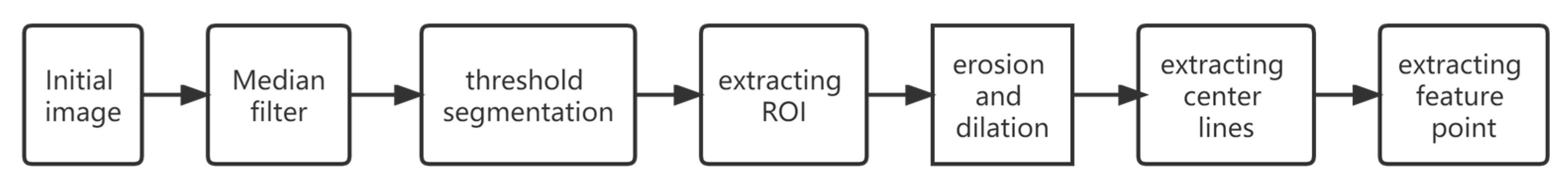
3.2. Image Preprocessing

After image binarization, the pixel value of the recognition area is retained, and the value of other areas of the image is 0. The processing process is shown in Figure 7a–c. After the structural light features are extracted by the neural network, in order to process the image faster and reduce the amount of data, we cut the ROI according to the size of the structural light region and divide the ROI region. For most image-processing projects, the ROI of each image is not necessarily in a fixed area, and even the size of the ROI area may be different. That is to say, the location and rectangular area of cutting should be determined according to each image.

First, the image is binarized, then the maximum connected domain of the whole region is extracted. After obtaining the maximum connected region, which is actually the region where the linear structured light is located, the point closest to the edge of the image in the connected domains of 0 degrees, 90 degrees, 180 degrees, and 270 degrees is found by traversing the entire image. Then, the whole connected area can be framed by creating a rectangular box using these four points; the ROI extraction effect is shown in Figure 7d.

3.3. Centerline Extraction

After obtaining the processed ROI image, in order to obtain the pixel coordinates of the weld feature point, P, we need to extract the center line of the linear structural light in the ROI area. According to the characteristics of the linear structural light on the right-angle weld, the intersection coordinates of the two linear structural lights will be the pixel coordinates of the weld feature point P after being restored to the original image. Coordinate extraction can be achieved via three steps: skeleton extraction, line extraction, and intersection coordinates.

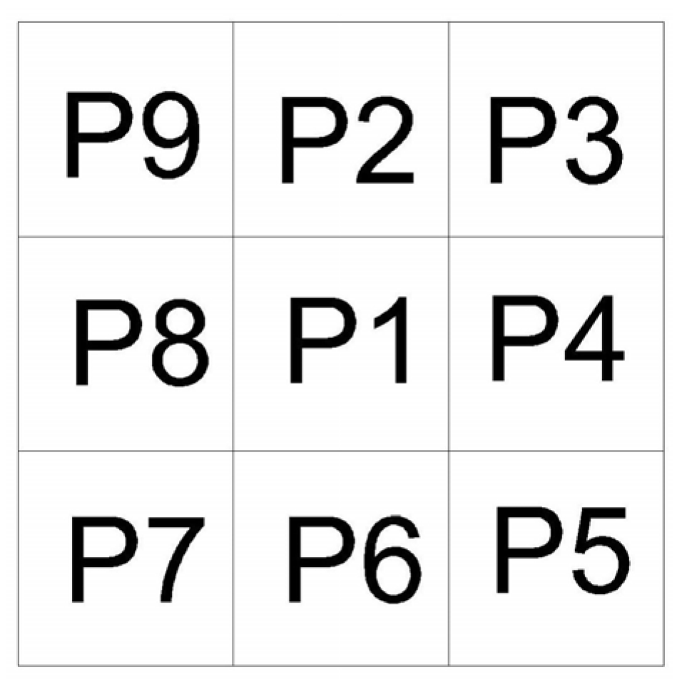
3.3.1. Skeleton Extraction

In the binarized image obtained after neural network segmentation, the structural light part will be broken due to the incomplete network recognition of the unrecognized part in Figure 7b,c and Figure 8, as well as the adaptive threshold of binarization (see Figure 7b), resulting in discontinuity of the line segment, as shown in the enlarged area of Figure 9a.

At present, the mainstream skeleton extraction methods generally include the Steger algorithm, refinement method, and gray centroid method. The gray centroid method is often used for butt welds because the fillet weld linear structural light cannot guarantee a fixed angle with the image boundary and cannot be processed by row and row pixels, so the gray centroid method is not applicable. The Zhang–Suen algorithm [25] is one representative refinement method. Thus, the Steger algorithm and Zhang–Suen algorithm were employed to extract the centerline of the image, and the extraction results are shown in Figure 9b,c, respectively. Under conditions of good recognition by the neural network, the extraction effect was better, but the extraction effect for discontinuous structural light was not efficient. The loss of discontinuous interval information would affect the extraction of weld feature points in the next step.

In order to eliminate the influence of discontinuity, the closed operation method was adopted, based on the operation of dilation, corrosion, etc., to carry out the closed operation of dilation before corrosion. Dilation can be used to filter the negative pulse noise in the image.

Let f(x) and g(x) be two discrete functions, defined for the two-bit discrete spaces F and G, where f(x) is the input image and g(x) is the structural element. Then, the dilation and corrosion of f(x) and g(x) are defined as:

$$(f\oplus g)(x)=\underset{y\in G}{\max }[f(x-y)+g(y)]$$

(5)

$$(f\Theta g)(x)=\underset{y\in G}{\min }[f(x+y)-g(y)].$$

(6)

The closing operation of f(x) with respect to g(x) is defined as:

$$(f•g)(x)=[(f\oplus g)\Theta g](x).$$

(7)

The results of the closing operation are shown in Figure 9e. The structural element used is a regular octagon, and the distance from the edge to the center is 15 pixels. At the beginning of the closing operation, a black edge of 20 pixels to the edge of the image was added, to prevent the target pixel from being too close to the edge and having an influence. The output aim is to remove the black edge. It can be seen from Figure 9e that the closing operation eliminates the influence of the discontinuity of part of the structural light. It is clear that the closing operation is useful for the extraction of discontinuous region information, so our general idea is the method of closing operation and centerline extraction. The Steger algorithm was used to extract the center line of Figure 9e, and its effect is shown in Figure 9f. We can see that the extraction effect is relatively good, but the calculation process of the Steger algorithm using a Hessian matrix is complicated. As shown in Equation (8), a second partial derivative of each pixel in four directions is needed.

$$H\left(x,y\right)=\left[\begin{array}{cc}{r}_{xx}& r_{xy}\\ r_{yx}& r_{yy}\end{array}\right]$$

(8)

There is a large amount of data to be processed. As shown in

Table 3. Comparison of the results.

Type	Morphological Erosions	Steger	Zhang–Suen	Closing Operation Steger	Dilation Zhang–Suen
Time (s)	0.0128	0.0877	0.0361	0.1035	0.0477
Discontinuous area identification length	_______	285.2087	336.9275	319.8760	354.5796

, the closing operation, combined with the Steger algorithm, takes 0.1753 s, which is a relatively long time. At this point, the closing operation method plus the Zhang–Suen algorithm was adopted. Since the closing operation is a combination of dilation corrosion operations, and the Zhang–Suen algorithm is also a corrosion operation, we tried to directly combine dilation and the Zhang–Suen algorithm into a new closed operation. The closed operation structure-function that we used before was a regular octagon, with a distance of 15 pixels from the edge to the center. Since the corrosion was deleted pixel by pixel, a smaller structure-function could be used in the dilation operation to reduce unnecessary calculations; therefore, the structure-function used in the dilation operation was a regular octagon with a distance of 10 pixels from the edge to the center. The structure-function g(x) of the Zhang–Suen corrosion algorithm is shown in Figure 10. P1 is the target pixel, and P2–P9 are numbered clockwise from the point above P1. In the first step, it is only when P1–P9 meets the condition of Equation (9) that it will be marked for deletion:

$$\left\{\begin{array}{c}2\le m(P_1)\le 6\\ n(P_1)=1\\ P_2\times P_4\times P_6=0\\ P_4\times P_6\times P_8=0\end{array}\right.$$

(9)

where $m\left(P_1\right)$ is the number of non-zero elements in the P2–P9 elements, and $n\left(P_1\right)$ is the number of mode 01 elements in the queue, arranged in order from P2 to P9. In the second step, it is only when P1–P9 meets the condition of Equation (10) that it will be marked for deletion:

$$\left\{\begin{array}{c}2\le m(P_1)\le 6\\ n(P_1)=1\\ P_2\times P_4\times P_8=0\\ P_2\times P_6\times P_8=0\end{array}\right..$$

(10)

We then cycle the above two steps until no pixel has been marked for deletion in both steps. The number of iterations is set as 35 times in this paper.

The output result yields the skeleton after image refinement, as shown in Figure 9g. It can be seen that the closing operation, combined with the Zhang–Suen algorithm, has a better effect on the discontinuous region than the conventional closed operation, and the extracted centerline information is also the most effective.

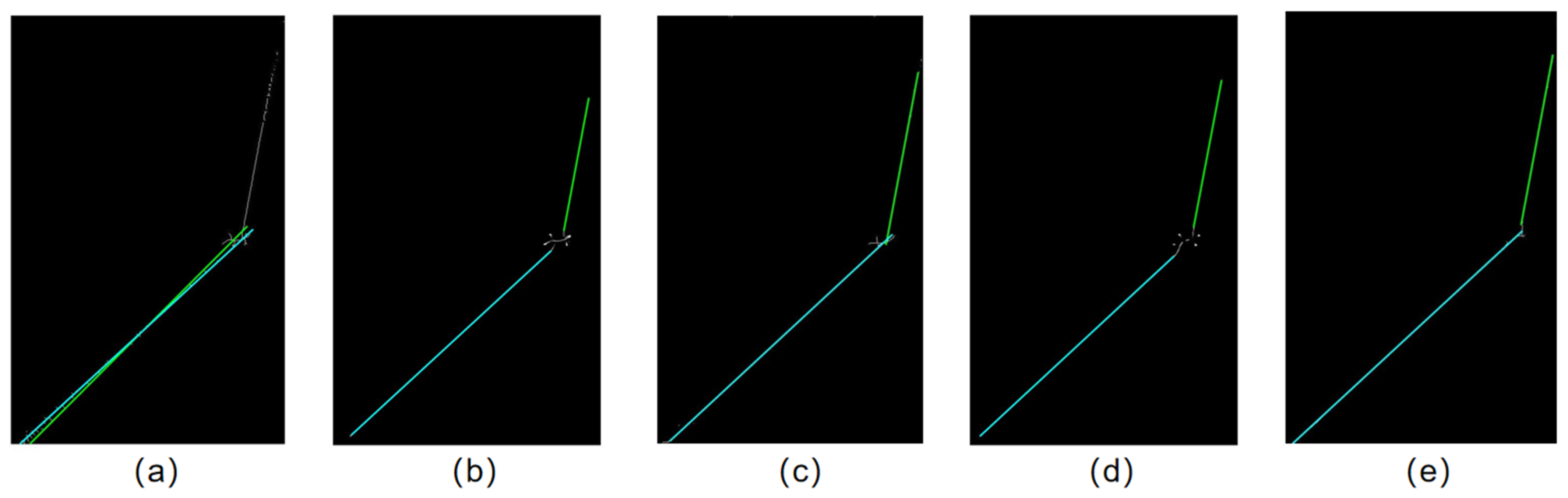
3.3.2. Line Extraction

After the linear-structured light skeleton is extracted, the Hough transform line detection method is adopted to transform the image from the image space to the parameter space. The transformation formula is shown in Equation (11):

$$y=kx+b\Rightarrow y=\frac{-\cos \theta }{\sin \theta }x+\frac{\rho }{\sin \theta }\Rightarrow \rho =x\cos \theta +y\sin \theta .$$

(11)

After the transformation, the relationship between the image space and parameter space is as follows: a point in the image space is a curve in the parameter space, and each collinear point in the image space corresponds to each curve where the parameter space intersects at a point. When the x and y values meet $\mathrm{r}=x·\cos \theta +y·\sin \theta$ in traversing the image, this point is considered to be a point on the detected line.

The spacing theta of the Hough transform along the θ-axis, the range of which is [−90, 89], was set to 0.2, while the interval of RhoResolution of the Hough transform along the ρ-axis was set to 0.5. The Hough space corresponding to the input image matrix was obtained. The number of intersecting points of curves in the Hough space were counted. By setting the minimum threshold of the statistics count to 0.3 times that of the maximum number of statistics, where the threshold = 0.3MAX, short lines were prevented from being detected.

By setting the threshold of the statistical number, the two lines corresponding to the two points with the largest statistical value are the required two lines of structural light, $l_1$ and $l_2$, where they set the parameter minlength = 150 for minimum line detection, and the parameter minlinegap = 20 for minimum line spacing; that is, when the distance between lines is less than 20, two lines will be merged. The final line extraction effect of these methods is shown in Figure 11. The images correspond to Hough space as shown in Figure 12.

In order to compare the applicability of each method, the methods were evaluated from two aspects. In the first instance, the processing time was used. The neural network processing in the previous step consumed a great deal of data-processing time. In order to obtain as large a welding speed interval as possible, the processing time of a single image should be as short as possible. In the second instance, the effect of straight-line extraction after skeleton extraction was analyzed. The more structural light information that was extracted, the more accurate the positioning. The distance between the longest point identified in the discontinuous region using each method and the intersection of two straight lines was measured. The longer the distance, the more information this method could extract from the discontinuous region, and the better the effect. The measurement results are shown in Table 3. Compared with the original algorithm, the recognition ability of the improved algorithm was improved. Compared with the closed operation that was combined with the Steger algorithm, the dilation combined with the Zhang–Suen algorithm used in this paper had a faster processing speed and better extraction effect on the discontinuous regions of structured light, at the cost of a little precision. Therefore, dilation, combined with the Zhang–Suen algorithm, is more suitable for the welding-seam positioning system in this paper.

3.4. Extraction of the Key Feature Points

In order to identify and position the diagonal welds well, we need to know the position of the weld point P; at the same time, in order to obtain a better welding torch angle for the laser head and the attitude at the end of the robot arm, the position attitude and included angle of the welded sheets A and B need to be identified. The attitude of the plate can be obtained through the coordinates of any two points on the two continuous structural lights. In Section 3.3.2, we calculated the $l_1$ and $l_2$ values of the structural light in the image coordinate system, and the intersection coordinates of the two lines were the weld feature point P. Equations (12) and (13) explain how the two lines were denoted.

$$l_1:a_1\cdot x_{l_1}+b_1\cdot y_{l_1}+c_1=0 (x_{l_1\min }<x_{l_1}<x_{l_1\max })$$

(12)

$$l_2:a_2\cdot x_{l_2}+b_2\cdot y_{l_2}+c_2=0 (x_{l_2\min }<x_{l_2}<x_{l_2\max })$$

(13)

The coordinate of the weld feature point P ($x_P,y_p$) is:

$$x_p=(b_1\cdot c_2-b_2\cdot c_1)/Z$$

(14)

$$y_p=(a_2\cdot c_1-a_1\cdot c_2)/Z$$

(15)

$$Z=a_1\cdot b_2-a_2\cdot b_1.$$

(16)

A new coordinate system was established, with the P coordinate as the origin, and the original line $l_1$ becoming that described in Equation (17).

$$l_1{}^{\prime }:a_1\cdot (x_{l_1}-x_p)+b_1\cdot (y_{l_1}-y_P)+c_3=0$$

(17)

In the new range of $l_1^{\prime }$, the point $x_a$ with the largest absolute value is taken, and the corresponding point $P_a\left(x_a,y_a\right)$ is the point farthest from the feature point P on the line $l_1$. Similarly, the point $P_b\left(x_b,y_b\right)$ on line $l_2$ can be obtained. The effects of the three extracted feature points P, $P_a$ and $P_b$ on the image are shown in Figure 13. According to the image coordinates, the three-dimensional coordinates of the $P_a$ and $P_b$ points on the plate are obtained. According to the coordinates of the two groups of P, $P_a$, and $P_b$, the position attitude and the included angle of sheet A and sheet B are obtained, so as to adjust the position attitude and the laser beam incidence angle. The farther that $P_a$ and $P_b$ are from P, the smaller the error is, and the more accurate the included angle between the plates that is obtained.

4. Welding Torch Attitude

In the process of welding-seam tracking, it is necessary to pay attention to the adjustment of the welding torch attitude and the distance between the end of the welding torch and the welding point, so as to avoid a collision between the welding torch and the welded part, and to ensure the quality of welding at the same time.

In Section 3.4, the three-dimensional coordinates of the feature point P of the weld and the $P_a$ and $P_b$ on the two sheets were calculated. Based on the two sets of such data, we can obtain the attitude of the welding torch. The mathematical model of the welding torch angle [26] is shown in Figure 14. The first set of data for $P_{A1}\left(X_{A1},Y_{A1},Z_{A1}\right), P\left(X_1,Y_1,Z_1\right),P_{A2}\left(X_{A2},Y_{A2},Z_{A2}\right),$ and the normal vector of sheet A and sheet B, are shown in Equations (18)–(20):

$$\stackrel{\rightharpoonup }{n_1}=P_1{P}_{A1}\times P_1{P}_{A2}=\left(a_1,b_1,c_1\right)$$

(18)

$$\stackrel{\rightharpoonup }{n_2}=P_1{P}_{B1}\times P_1{P}_{B2}=\left(a_2,b_2,c_2\right)$$

(19)

$$\stackrel{\rightharpoonup }{n_3}=\stackrel{\rightharpoonup }{n_1}\times \stackrel{\rightharpoonup }{n_2}=\left(a_3,b_3,c_3\right)$$

(20)

where $\stackrel{\rightharpoonup }{n_3}$ represents the direction vector from P₁ to P₂, namely, the tangent vector in the direction of weld travel. Plane C is the plane perpendicular to sheet A and sheet B, passing through point P₁. The Z-axis of the laser coordinate system is on this plane, and the direction vector of the Z-axis bisects the dihedral angle between sheet A and sheet B. The expression of plane C is shown in Equation (21).

$$a_3\left(X-X_1\right)+b_3\left(Y-Y_1\right)+c_3\left(Z-Z_1\right)=0$$

(21)

$$\stackrel{\rightharpoonup }{n_{CA}}=\stackrel{\rightharpoonup }{n_1}\times \stackrel{\rightharpoonup }{n_3}$$

(22)

$$\stackrel{\rightharpoonup }{n_{CB}}=\stackrel{\rightharpoonup }{n_2}\times \stackrel{\rightharpoonup }{n_3}$$

(23)

$\stackrel{\rightharpoonup }{n_{CA}}$ is the direction vector of the intersection line between plane C and sheet A, and $\stackrel{\rightharpoonup }{n_{CB}}$ is the direction vector of the intersection between plane C and sheet B. The unit vectors are $e_{CA}$ and $e_{CB}$:

$$e_{\frac{\theta }{2}}=e_{CA}+e_{CB}$$

(24)

$$P_{laser}=P_1+k\cdot e_{\frac{\theta }{2}}$$

(25)

where $P_{laser}$ is the end coordinate of the manipulator after attitude modification; the Z-axis of the end coordinate system is $-e_{\frac{\theta }{2}}$, and k is the proportional coefficient of the distance between the laser head and the laser intersection, which is 150 in the experiment. The welding torch attitude adjustment model is shown in Figure 15. The blue points are weld feature points, while the red and green points are $P_a$ and $P_b$, respectively. These three kinds of feature points constitute the three-dimensional contour of the entire irregular fillet weld. The vector shown by the arrow is $\stackrel{\rightharpoonup }{n_{\frac{\theta }{2}}}$, pointing from the weld feature point to the origin of the coordinate system of the end of the manipulator, corresponding to the weld feature point. Welding along the modified welding-torch attitude can complete the welding of irregular welds, avoid the collision between the welding torch and the workpiece, and adjust the welding torch angle to achieve better welding quality.

5. Experiment and Analysis

In order to verify the weld identification and positioning system designed in this paper, it was necessary to conduct a weld-positioning experiment. The experimental platform shown in Figure 16 and a welded part made of 304 stainless steel were used to test the identification and positioning performance of the proposed method in the context of a downline structural light with high mirror-reflection effect. At the same time, in order to check that this method can correct the attitude of the torch and effectively avoid collision with the welded parts, a Z-shaped bending structure of 90° fillet-welded stainless steel plate was selected for testing.

The experimental steps of high-mirror reflector structured light location are as follows:

• Check the surrounding environment of the welding robot, confirm that the barrier is free, and begin the experiment. Install the auxiliary positioning tool shown in Figure 17; the vertex of the positioning tool is the focus position of the laser beam and it is also the most ideal position for the laser to hit the weld. At this time, images of weld are collected to obtain the initial weld feature points. If the acquisition fails at this point, repeat the previous steps.
• Set the moving speed of the welding robot and start the program. During operation, the laser head laser should always move with the welding seam and change the robot’s attitude in real time. When moving to the end of the workpiece, the program ends; save the position coordinates of the feature points during the program, while it is running, for experimental analysis.

In view of the errors between the actual model and the theoretical model, as well as the welding part processing errors, in this paper, the contact measurement method was used to determine the control data of the experimental results. At this point, we selected the 4 vertices of any safe weld and any 6 points on the edge or surface of the plane on the welding part and switched the robot arm to the tool coordinate system. The repeated positioning accuracy of the robot arm was ±0.03 mm. We installed the positioning tool as shown in Figure 17, using the tool coordinate system to locate it, approached the selected points from different directions, recorded the five groups of effective data, and took the average value. The set of plane points was obtained, then least-squares plane fitting was carried out on these points to find the welding plane expression, so as to establish the mathematical model of the welding parts. We positioned the coordinates of points on the surface of the welding parts again and kept the error within 0.08 mm from the mathematical model of welding parts.

The plane intersection line of the welding-part model is the characteristic curve of the ideal weld, which was compared with the experimental data. We recorded the vertical distance between the feature points and the ideal weld characteristic curves in the y and z directions, the vertical distance between the PA and PB points and the fitting plane, and the difference between the angle of the plane, obtained by each set of data, and the angle between the model plane of welding parts. Fifty groups of experimental data were selected to be compared with the model and error data, as shown in Figure 18, Figure 19 and Figure 20, were obtained.

On the test piece, the maximum detection error of the weld feature point P in the Y-axis and Z-axis directions is 0.3347 mm and 0.3135 mm, respectively, and the average detection error are 0.1709 mm and 0.1768 mm, respectively. The maximum vertical error of the feature point P_a and P_b and the distance from board A and board B are 0.3876 mm and 0.4341 mm, respectively, while the average vertical error is 0.2152 mm and 0.2400 mm, respectively. The maximum angle error of the angle between plates is 0.3657°, and the average angle error is 0.1836°.

The method proposed in this paper was analyzed through experiments, then it was compared with the method proposed by the authors of [22] for calculating welding likelihood degree by a convolution kernel, as shown in

Table 4. Comparison of the test results between the weld likelihood method and the method in this paper.

Methods	Normal Fillet Weld	Highly Reflective Fillet Weld	Time per Picture	Maximum Error of Weld Feature Points	Maximum Angle between Plates
weld likelihood method	100%	100%	0.18 s	0.52 mm	______
method in this paper	100%	98.9%	0.23 s	0.35 mm	0.3657°

. The recognition rates of welds under different reflective conditions were tested. The recognition rates of the welding likelihood method and the method in this paper were both 100% in the ordinary fillet weld test, 100% in the case of the highly reflective fillet weld, and 98.9% in this paper. With highly reflective fillet welds, the average welding likelihood method takes 0.18 s per image, while the method proposed in this paper takes 0.23 s. However, the maximum positioning error of the welding likelihood method for weld feature points is 0.52 mm, while the proposed method in this paper is 0.35 mm. In this paper, the maximum angle error of the included angle between plates is 0.3657°. The weld likelihood degree method cannot be employed because it does not consider adjusting the attitude of the welding torch. In general, compared with the welding likelihood method, the proposed method is slightly lower in recognition accuracy and speed, and the positioning accuracy of the feature points is higher than that of the welding likelihood method, which can realize the attitude adjustment of the welding torch, a task that the welding likelihood method cannot accomplish.

The results show that the comprehensive positioning accuracy can reach 0.2471 mm, and the measurement accuracy of the attitude between plates can reach within 0.4°, which can realize the accurate identification and positioning of the welding seam and the attitude correction of the welding torch and meet the welding accuracy requirements of a stainless-steel right-angle weld.

6. Conclusions

In this paper, a neural network is proposed to filter the reflective noise in calculating images, and the feature points are reconstructed into a 3D model after image processing. The diagonal welds are identified and positioned, and the welding torch angle is corrected. Under conditions where the workpiece surface has high reflectivity and the weld shape is irregular, the problems of weld positioning and welding torch angle correction in the context of reflection noise are solved. The main contributions of this paper include:

(1)

A fillet weld positioning method is proposed that can effectively overcome the uneven reflection of linear structure light intensity;

(2)

A DeeplabV3+ model was used for the first time to identify linear structural light and to filter reflective noise, while MobileNetV2 was used as the backbone network to improve the efficiency of model recognition, compared with the traditional network model;

(3)

Based on the closed operation used in the TMM to eliminate the effect of binarization, the expansion, combined with the Zhang–Suen method, was used to extract the skeleton of the discontinuous region, which improved the ability to filter negative pulse noise. Compared with other mainstream skeleton extraction methods, the improved method was proven to be superior to the traditional method;

(4)

The attitude correction of a welding torch was studied, the three-dimensional reconstruction mathematical model of the system was established, and the coordinates of the welding seam and welding torch angle were obtained, according to the deduced formula;

(5)

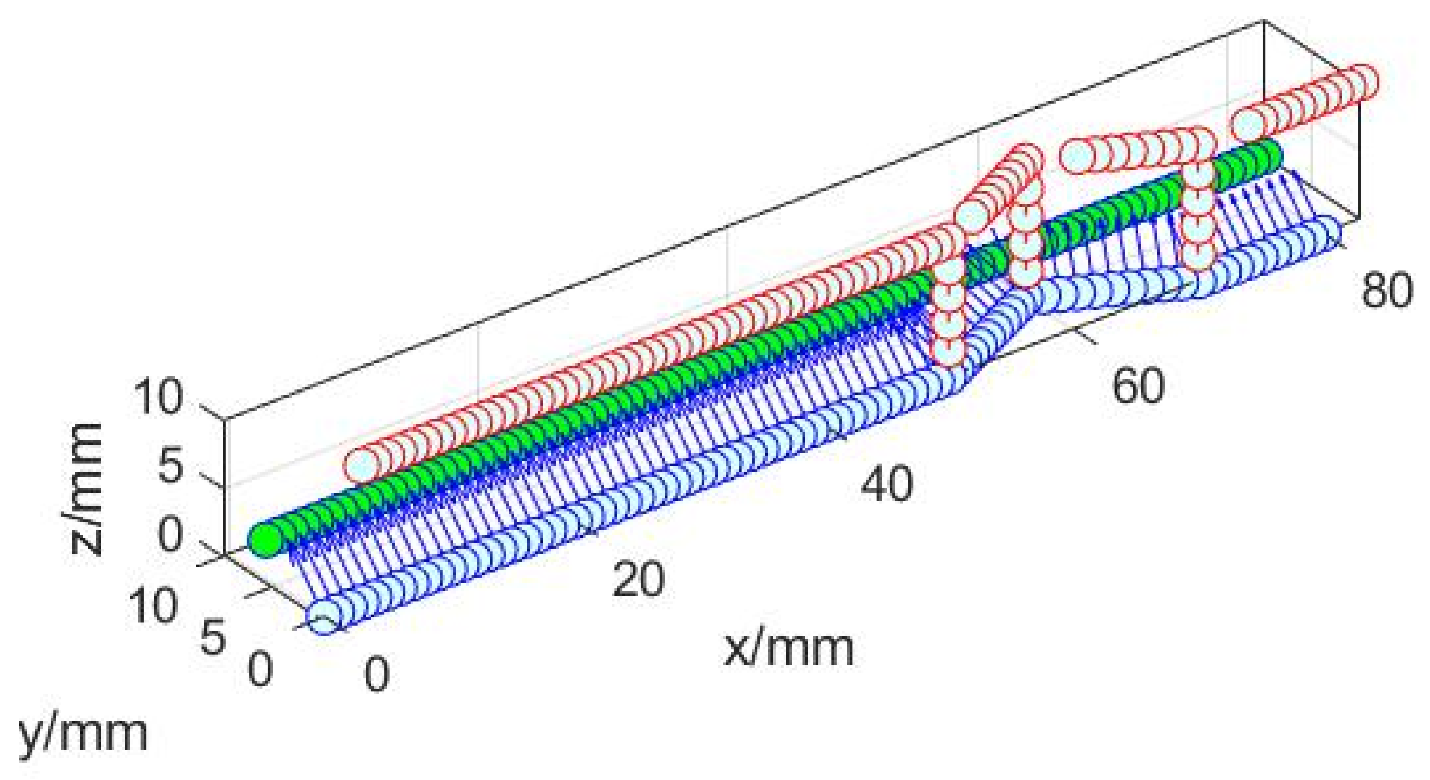
The positioning experiment was carried out on stainless steel and highly reflective irregular fillet welds. The experimental results showed that the identified weld feature points were continuous, and the welding torch angle was satisfactory, without collision. The average detection error of the weld feature point P in the Y-axis and Z-axis directions was 0.1709 mm and 0.1768 mm, respectively. The average angle error of the angle between sheets was 0.1836°. The accuracy of the weld identification model meets the requirements and verifies the effectiveness of the system.

In the experiment, the laser self-melting welding technique was used; the workpiece surface was free of oil, the protective atmosphere of argon was sufficient, and the welding splash was minimized. In future research, the proposed neural network needs to be further optimized under splash interference.

References

1. Rout, A.; Deepak, B.; Biswal, B.B. Advances in weld seam tracking techniques for robotic welding: A review, Robot. Comput. Integr. Manuf. 2019, 56, 12–37. [Google Scholar] [CrossRef]
2. Lei, T.; Rong, Y.; Wang, H.; Huang, Y.; Li, M. A review of vision-aided robotic welding. Comput. Ind. 2020, 123, 103326. [Google Scholar] [CrossRef]
3. Lee, D.; Ku, N.; Kim, T.W.; Kim, J.; Lee, K.Y.; Son, Y.S. Development and application of an intelligent welding robot system for shipbuilding, Robot. Comput. Integr. Manuf. 2011, 27, 377–388. [Google Scholar] [CrossRef]
4. Xia, C.; Pan, Z.; Polden, J.; Li, H.; Xu, Y.; Chen, S.; Zhang, Y. A review on wire arc additive manufacturing: Monitoring, control and a framework of automated system. J. Manuf. Syst. 2020, 57, 31–45. [Google Scholar] [CrossRef]
5. Yang, L.; Li, E.; Long, T.; Fan, J.; Liang, Z. A high-speed seam extraction method based on the novel structured-light sensor for arc welding robot: A review. IEEE Sens. J. 2018, 18, 8631–8641. [Google Scholar] [CrossRef]
6. Wang, B.; Hu, S.J.; Sun, L.; Freiheit, T. Intelligent welding system technologies: State-of-the-art review and perspectives. J. Manuf. Syst. 2020, 56, 373–391. [Google Scholar] [CrossRef]
7. Xue, K.; Wang, Z.; Shen, J.; Hu, S.; Zhen, Y.; Liu, J.; Wu, D.; Yang, H. Robotic seam tracking system based on vision sensing and human-machine interaction for multi-pass MAG welding. J. Manuf. Processes 2021, 63, 48–59. [Google Scholar] [CrossRef]
8. Maldonado-Ramirez, A.; Rios-Cabrera, R.; Lopez-Juarez, I. A visual path-following learning approach for industrial robots using DRL, Robot. Comput. Integr. Manuf. 2021, 71, 102130. [Google Scholar] [CrossRef]
9. Zou, Y.; Wang, Y.; Zhou, W.; Chen, X. Real-time seam tracking control system based on line laser visions. Opt. Laser. Technol. 2018, 103, 182–192. [Google Scholar] [CrossRef]
10. Bračun, D.; Sluga, A. Stereo vision based measuring system for online welding path inspection. J. Mater. Processing Technol. 2015, 223, 328–336. [Google Scholar] [CrossRef]
11. Ding, Y.; Huang, W.; Kovacevic, R. An on-line shape-matching weld seam tracking system. Robot. Comput. Integr. Manuf. 2016, 42, 103–112. [Google Scholar] [CrossRef]
12. Li, X.; Li, X.; Khyam, M.O.; Ge, S.S. Robust welding seam tracking and recognition. IEEE Sens. J. 2017, 17, 5609–5617. [Google Scholar] [CrossRef]
13. Xue, B.; Chang, B.; Peng, G.; Gao, Y.; Tian, Z.; Du, D.; Wang, G. A vision based detection method for narrow butt joints and a robotic seam tracking system. Sensors 2019, 19, 1144. [Google Scholar] [CrossRef] [PubMed] [Green Version]
14. Dinham, M.; Fang, G. Autonomous weld seam identification and localisation using eye-in-hand stereo vision for robotic arc welding. Robot. Comput.-Integr. Manuf. 2013, 29, 288–301. [Google Scholar] [CrossRef]
15. Ma, H.; Wei, S.; Sheng, Z.; Lin, T.; Chen, S. Robot welding seam tracking method based on passive vision for thin plate closed-gap butt welding. Int. J. Adv. Manuf. Technol. 2010, 48, 945–953. [Google Scholar] [CrossRef]
16. HShah, N.M.; Sulaiman, M.; Shukor, A.Z.; Kamis, Z.; Rahman, A.A. Butt welding joints recognition and location identification by using local thresholding. Robot. Comput.-Integr. Manuf. 2018, 51, 181–188. [Google Scholar] [CrossRef]
17. Shao, W.; Liu, X.; Wu, Z. A robust weld seam detection method based on particle filter for laser welding by using a passive vision sensor. Int. J. Adv. Manuf. Technol. 2019, 104, 2971–2980. [Google Scholar] [CrossRef]
18. Dinham, M.; Fang, G. Detection of fillet weld joints using an adaptive line growing algorithm for robotic arc welding. Robot. Comput.-Integr. Manuf. 2014, 30, 229–243. [Google Scholar] [CrossRef]
19. Du, R.; Xu, Y.; Hou, Z.; Shu, J.; Chen, S. Strong noise image processing for vision-based seam tracking in robotic gas metal arc welding. Int. J. Adv. Manuf. Technol. 2019, 101, 2135–2149. [Google Scholar] [CrossRef]
20. Yu, W.; Li, Y.; Yang, H.; Qian, B. The Centerline Extraction Algorithm of Weld Line Structured Light Stripe Based on Pyramid Scene Parsing Network. IEEE Access 2021, 20, 105144–105152. [Google Scholar] [CrossRef]
21. Zhao, Z.; Luo, J.; Wang, Y.; Bai, L.; Han, J. Additive seam tracking technology based on laser vision. Int. J. Adv. Manuf. Technol. 2021, 116, 197–211. [Google Scholar] [CrossRef]
22. Chen, S.; Liu, J.; Chen, B.; Suo, X. Universal fillet weld joint recognition and positioning for robot welding using structured light. Robot. Comput.-Integr. Manuf. 2022, 74, 102279. [Google Scholar] [CrossRef]
23. Chen, L.C.; Zhu, Y.; Papandreou, G.; Schroff, F.; Adam, H. Encoder-decoder with Atrous separable convolution for semantic image segmentation. In Proceedings of the 15th European Conference on Computer Vision, Munich, Germany, 8–14 September 2018; pp. 833–851. [Google Scholar]
24. Sandler, M.; Howard, A.; Zhu, M.; Zhmoginov, A.; Chen, L.C. MobileNetV2: Inverted residuals and linear bottlenecks. In Proceedings of the 2018 IEEE/CVF Conference on Computer Vision and Pattern Recognition, Salt Lake City, UT, USA, 18–23 June 2018. [Google Scholar]
25. Zhang, T.Y.; Suen, C.Y. A fast parallel algorithm for thinning digital patterns. Commun. ACM 1984, 27, 236–239. [Google Scholar] [CrossRef]
26. Mei, L.; Yan, D.; Chen, G.; Wang, Z.; Chen, S. Influence of laser beam incidence angle on laser lap welding quality of galvanized steels. Opt. Commun. 2017, 402, 147–158. [Google Scholar] [CrossRef]
Figure 1. The traditional morphological method (TMM) process.
Machines 11 00038 g001
Figure 2. The weld positioning system.
Machines 11 00038 g002
Figure 3. Flow chart of the experiment.
Machines 11 00038 g003
Figure 4. A 3D reconstruction model of the linear structured light.
Machines 11 00038 g004
Figure 5. The DeeplabV3+ structure diagram.
Machines 11 00038 g005
Figure 6. The image processing results of the different models.
Machines 11 00038 g006
Figure 7. Image-processing flow after neural network segmentation. (a) original image (b) binarization (c) image after recognition by the neural network (d) ROI extraction.
Machines 11 00038 g007
Figure 8. Line-structured light identifies the discontinuous regions.
Machines 11 00038 g008
Figure 9. (a) Original figure; (b) with the Steger algorithm; (c) with the Zhang–Suen algorithm; (d) morphological corrosion results; (e) the closing operation; (f) the closing operation, combined with the Steger algorithm; (g) dilation, combined with the Zhang–Suen algorithm.
Machines 11 00038 g009
Figure 10. The target pixel and its neighborhood.
Machines 11 00038 g010
Figure 11. Linear extraction results after various skeleton extraction algorithms: (a) morphological erosions; (b) the Steger algorithm; (c) the Zhang–Suen algorithm; (d) closing operation with the Steger algorithm; (e) dilation with the Zhang–Suen algorithm.
Machines 11 00038 g011
Figure 12. Dilation, combined with Zhang–Suen algorithm, corresponding to the Hough space.
Machines 11 00038 g012
Figure 13. Extraction of the weld feature points.
Machines 11 00038 g013
Figure 14. Mathematical model of the welding-torch positioning.
Machines 11 00038 g014
Figure 15. Model of the weld feature points and welding-torch angle. The red point is the feature point on sheet A, the green point is the feature point on sheet B, the light blue point is the weld feature point, and the dark blue arrow is the direction vector of the weld feature point pointing to axis Z of the sixth axis of the manipulator.
Machines 11 00038 g015
Figure 16. The experimental platform.
Machines 11 00038 g016
Figure 17. The auxiliary positioning tool.
Machines 11 00038 g017
Figure 18. Errors in the weld feature points in the Y and Z directions.
Machines 11 00038 g018
Figure 19. The positioning errors of P a and P b .
Machines 11 00038 g019
Figure 20. The weld angle error.
Machines 11 00038 g020