Article

Trajectory Control Strategy and System Modeling of Load-Sensitive Hydraulic Excavator

Shanghai Key Laboratory of Intelligent Manufacturing and Robotics, School of Mechatronic and Automation Engineering, Shanghai University, Shanghai 200444, China
*
Author to whom correspondence should be addressed.
Machines 2023, 11(1), 10; https://doi.org/10.3390/machines11010010
Submission received: 15 November 2022 / Revised: 16 December 2022 / Accepted: 18 December 2022 / Published: 22 December 2022
(This article belongs to the Section Automation and Control Systems)

Abstract

:
Accurate control of excavator trajectory is the foundation for the intelligent and unmanned development of excavators. The excavator operation process requires multiple actuators to cooperate to complete the response action. However, the existing control methods to realize a single actuator of the excavator can no longer meet the practical demand. Based on this, a hybrid adaptive quantum particle swarm optimization algorithm (HAQPSO) is proposed to tune the proportional integral derivative (PID) controller parameters for enhancing the trajectory control accuracy of excavator actuators. To increase particle randomization and search speed and avoid the local convergence of QPSO, the QPSO is combined with circle chaotic mapping, Gaussian mutation operators, and adaptive adjustment factors, while the linear transformation of the contraction-expansion coefficient (CE) is improved to the dynamic adjustment mode. Through the interface block, a co-simulation platform for the load-sensitive system excavator is constructed, and trajectory experiments of multiple actuator compound actions are carried out. The simulation results show that—compared with ZN-PID, PSO-PID, and QPSO-PID—the trajectory error accuracy of the boom is improved by 26.59%, 32.95%, and 9.44%, respectively, which proves the high control accuracy of HAQPSO-PID in controlling the trajectory of multiple actuators.

1. Introduction

Hydraulic excavators, as typical multifunctional construction machinery, are indispensable in energy exploitation, road building, infrastructure construction, and many other fields [1]. However, hydraulic excavator systems are complex electromechanical–hydraulic integrated systems with nonlinear and multi-constrained characteristics. Meanwhile, dead zones, valve hysteresis, fluid leakages and mechanical wear of hydraulic valves lead to certain delays and errors in the trajectory control of hydraulic actuators [2]. The actuators on a classic excavator are controlled by a professional operator using joysticks, and the digging operation is completed based on his observations. With this operation method, automatic and precise trajectory control is no longer possible.
The foundation of unmanned excavators is accurate trajectory control. The excavator, unlike indoor mechanical robotics, is operated in a harsh environment with complex circumstances and severe interference [3]. Hence, how to realize the accurate control of the operation trajectory through a simple control strategy has become a hot topic in excavator automation research. Many approaches have been proposed to handle this issue, including proportional integral derivative (PID) [4], fuzzy control [5], robust control [6], sliding mode control [7], and so on. In addition, adaptive control methods are also available and widely used in electrohydraulic servo systems [8,9]. Although many methods can achieve satisfactory control results, some methods are difficult to implement in engineering practice because of their complex structure and dependence on model parameters. Furthermore, multiple actuators controlled by a single hydraulic pump cause nonlinear and time variability in excavator hydraulic systems, which makes it challenging to accurately establish the excavator control model.
In the field of industrial control, new control approaches have emerged. Nevertheless, PID continues to be used by more than 90% of controllers due to its simple structure, easy implementation, and high stability [10,11]. Due to the limitations of cost and working conditions, trajectory control of the excavator is mainly realized by the PID controller. To improve the tracking accuracy of a micro excavator, Zhang proposed a flow-rate-matching feedforward plus PID control approach for a zonal hydraulic system of off-road machinery. The control method has good position track accuracy, and its root mean square error (RMSE) was reduced by 20–87% in simulation experiments [12]. Tri investigated a fused fractional-order fuzzy logic and PID controller for electrohydraulic rotary actuator trajectory control, and the performance of the controller was analyzed in co-simulation experiments [13]. PID control parameters affect the stability, accuracy, and speed of the system. Additionally, the parameter adjustment process of standard PID controllers is complex and time-consuming. In recent years, particle swarm optimization (PSO) [14,15], fuzzy optimization [16], genetic optimization (GA) [17] and other optimization algorithms have been applied to tune PID parameters. Optimization algorithms are used to achieve the optimal search of PID parameters, reduce the difficulty of tuning PID parameters, and enable the PID controller to meet the control requirements.
PSO is also a swarm intelligence algorithm, which uses the power of a swarm to find the optimal solution of the problem as much as possible. The search performance is comparable to other optimization algorithms, such as ant colony optimization (ACO). PSO has the advantages of few parameters, simple software programming, and fast convergence. Some new population intelligence algorithms, such as the sparrow search algorithm (SSA) [18], the Aquila optimizer (AO) [19] and others have changed in the optimal individual updating mode, but their essence remains the population optimization method. These evolutionary algorithms have been widely used in engineering fields. However, Van den Bergh proved that PSO is not a global convergence algorithm [20]. To achieve global optimization, quantum particle swarm optimization (QPSO) was proposed to improve the global search capability of PSO. It preserves the benefits of the PSO algorithm, eliminates particle velocity and location limitations, reduces parameter settings, and improves algorithm randomness. On several benchmark test functions, the results reveal that the global search performance of QPSO outperforms that of ordinary PSO. Nevertheless, local convergence and loss of variety are still drawbacks of QPSO. Therefore, since the QPSO algorithm was put forward, numerous scholars have optimized, refined, and applied it widely.
A load-sensitive (LS) system is a closed-center hydraulic system, which is different from open-center hydraulic systems in terms of negative flow control and positive flow control. On the basis of the original valve control system, the flow-adjustable pump is added to form a pump control pressure system, which successfully overcomes the problem of median throttling loss in the open-center hydraulic system. The constant pressure difference before and after the multiway valve is achieved by a pressure compensation valve [21]. The flow to the actuator element is independent of its loads, and is only related to the spool opening of the multiway valve spool, which ensures the good handling performance of the excavator during compound action. Although the energy economy and response speed of the LS system are taken into account to some extent, the linkage of pump control and valve control in the LS system makes accurate control trajectory more challenging.
Although considerable research has been done on the trajectory control of excavator actuators, most of it has focused only on the open-center hydraulic system under the valve control system, and there have been few studies on the trajectory control of LS excavators with the combination of pump control and valve control. Furthermore, most of the research is devoted to single-actuator trajectory control such as bucket, rather than the trajectory control of all actuators in compound operation.
To enable the automatic control of multi-actuator compound operation trajectory automatic control in the hydraulic excavator. A parameter-tuning PID controller based on the hybrid adaptive QPSO algorithm (HAQPSO-PID) is proposed to improve the control accuracy of the excavator actuator trajectory. Chaotic mapping and Gaussian mutation operators are added to the classic QPSO algorithm to improve particle randomness. The linear transformation of the contraction–expansion coefficient (CE) is transformed into a dynamic adjustment mode to avoid local convergence, and the randomly generated factor is tuned for adaptive adjustment. HAQPSO efficiently improves the trajectory of multiple actuators under the compound operation by integrating QPSO with Gaussian variation, chaotic mapping, and adaptive adjustment. The LS excavator co-simulation model is established and the accuracy of the co-simulation model is verified by real data of an excavator. Furthermore, the trajectory control experiment of an LS excavator with multiple actuators is carried out through the co-simulation model, and the trajectory control accuracy of excavators under different PID controllers is compared.
The rest of the paper is organized as follows. The LS excavator working principle is analyzed in Section 2. Section 3 establishes the pump control and valve control model of the excavator. Section 4 provides the PID parameter-tuning method based on HQPSO. Section 5 constructs the co-simulation model of the LS excavator. Section 6 presents the comparative experimental results of trajectory comparison under different control methods. Finally, the paper is concluded in Section 7.

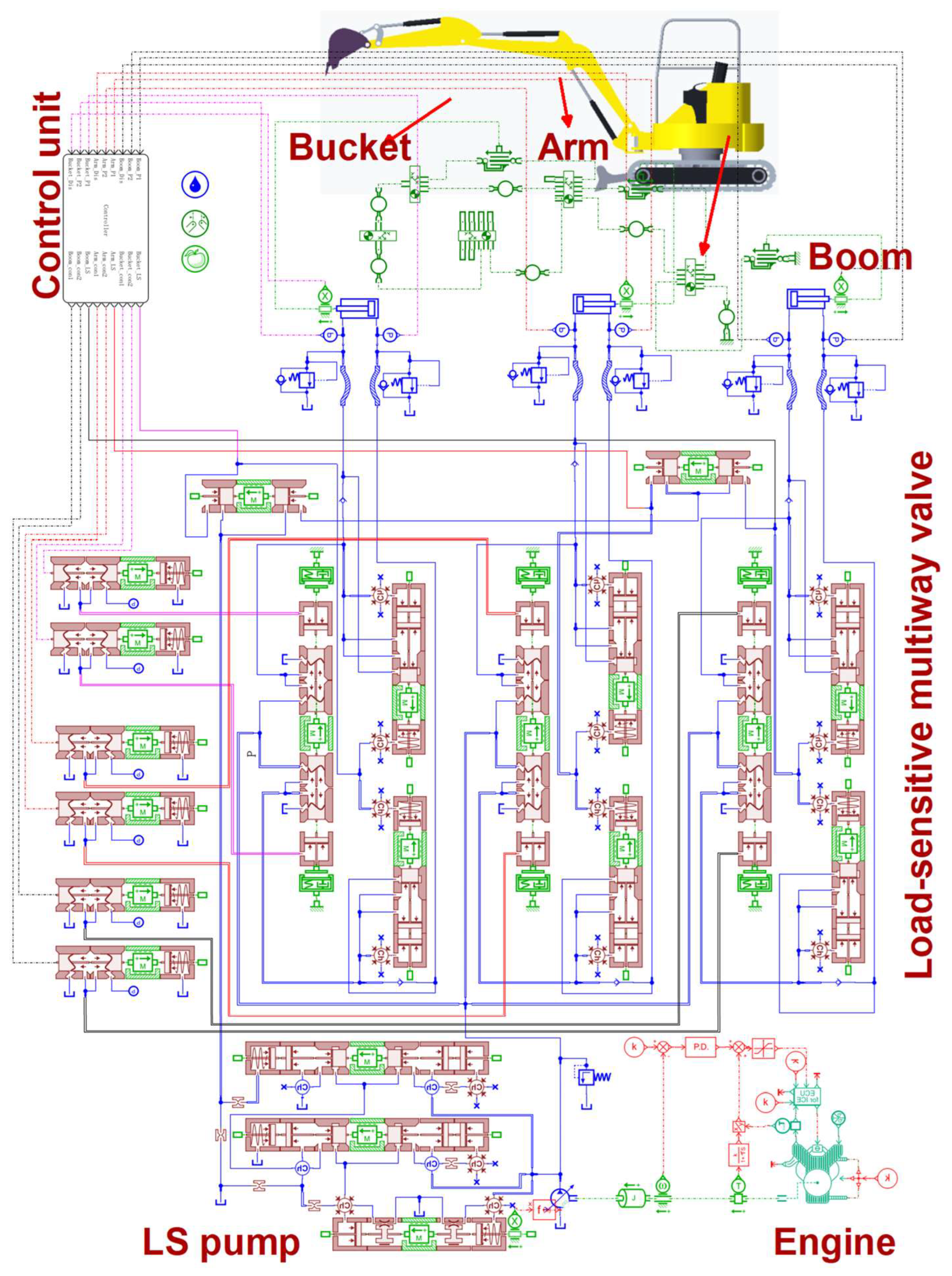
2. Hydraulic Excavator System Analysis

The hydraulic system of the excavator analyzed in this paper is the LS system, and the hydraulic schematic is shown in Figure 1. Displacement sensors, pressure sensors, flow meters, controllers, and other equipment are installed to collect the operating characteristics of excavator in real time. The valve control subsystem consists of actuators (boom, arm, bucket), displacement sensors, controller, and multiway valve. The diesel engine, variable pump, pressure sensors, and controller establish the pump control subsystem. Among them, the pump control subsystem controls the pump outlet pressure at a value higher than the load pressure to achieve load-sensitive control functions and reduce throttling and overflow losses [22]. The excavator trajectory is controlled by the valve control subsystem. The whole operation process of the excavator is realized by the cooperation of the valve control subsystem and the pump control subsystem. The control flowchart of the LS hydraulic excavator system is shown in Figure 2.
During the actuator operation, the pressure signal loaded by the actuator is fed back to the spring chamber of the multiway valve pressure compensator in real time, and the pressure compensation is realized by the pressure compensator valve.
The differential pressure at both ends of the throttle port remains constant, and the throttle opening of the multiway valve determines the actuator flow rate, regardless of its load. When multiple actuators are operated, the maximum load pressure of actuators is detected by the shuttle valve and fed back to the control port of the variable pump. Concurrently, the rotation angle of the pump is adjusted to supply only the flow and pressure required by the actuators, and the throttling and overflow loss are effectively reduced. Even if the load pressure of multiple actuators is different, the multiple actuators can still be controlled quickly and precisely simultaneously, and the actuators can be guaranteed not to interfere with each other.

3. LS Excavator Systematic Modeling

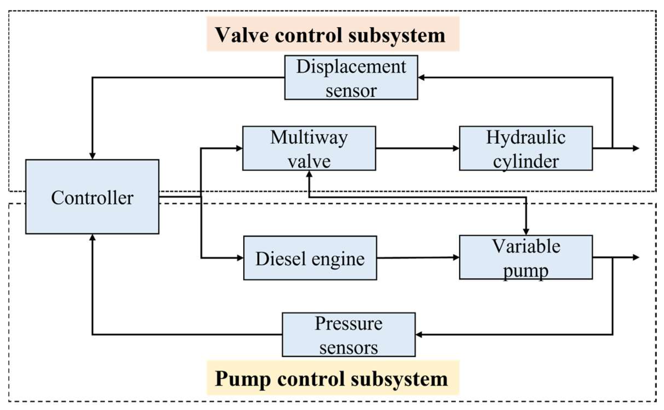
3.1. Valve Control Subsystem Modeling

In the valve control subsystem, the trajectory control of the actuator entails the following processes: (1) the desired trajectory signal controls the pilot valve through joysticks, (2) the hydraulic signal of the pilot valve controls the multiway valve, (3) the multiway valve controls the hydraulic cylinder to perform the corresponding actions, and (4) the trajectory signal is fed back to the controller.

3.1.1. Joystick to Pilot Valve

During excavator operation, the driver operates the joystick to deliver directions according to the desired trajectory, and the joystick pressure-reducing valve adjusts the spool displacement to vary the output pressure depending on the joystick angle. Based on a sample excavator manual, the control equation of the joystick is:
P c ( θ ) = { 0 0 θ 2.5 7 6 ( θ 2.5 ) + 5 2.5 < θ < 17.5 40 17.5 θ 19
where θ is the joystick angle and P c is the output pressure.
The flow equation and force balance equation of the pilot valve are:
{ x p l K p l = P c Q p l = K p q x p l K p v P p v
where x p l is the pilot valve spool displacement, K p l , K p q and K p v are the pilot valve spring stiffness, flow coefficient, and flow pressure coefficient, respectively, and Q p l and P p v are the load pressure and load flow of pilot valve, respectively.

3.1.2. Pilot Valve to Multiway Valve

The structure of the multiway valve is shown in Figure 3. The hydraulic signal generated by the pilot valve acts on both sides of the multiway valve, and the opening area of the multiway valve is adjusted through the pilot pressure and the multiway valve reset spring to achieve throttling speed control.
The force balance equation and flow continuity equation of multiway valve can be given as:
{ P p v A p k v ( x 0 + x v ) = m d 2 x v d t 2 + B v d x v d t + k f x v Q p v = A p d x v d t + 1 2 C p P p v + V p 4 β d P p v d t
where x v is the displacement of the multiway spool, m is the mass of the multiway valve spool, k v is the spring stiffness, x 0 is spring precompression, k f is the fluid stiffness, A p is the control chamber area, B v is the viscous damping factor, C p is the leakage coefficient, and the main valve control pressure P p v is:
P p v = P a P b
The spool frequently reciprocates movements during operation, which results in internal leakage. Hence, the external leakage of the multiway valve is ignored and only the internal leakage is considered, the flow continuity equation of the two control chambers in the multiway valve is:
{ P a = A p d x v d t + C ( P a P t ) + V a β d P a d t P b = A p d x v d t + C ( P t P b ) + V b β d P b d t
where β is the elastic bulk modulus, V a and V b are the volumes at both sides of the multiway valve, respectively, and P t is the tank pressure.

3.1.3. Multiway Valve to Actuators

The bucket, arm and boom hydraulic cylinders of the excavator are all double-acting hydraulic piston actuators. The spool of the corresponding multiway valve moves as the excavator is operated, adjusting the overflow area. Its force balance equation is:
m c x ¨ c = A c ( P 1 P 2 ) B x ˙ c K c x c F l F f
where m c is the load mass, x c is the piston displacement, P 1 and P 2 are hydraulic chamber pressures, A c is the hydraulic cylinder effective action area, B and K c are the viscous friction damping coefficient and spring stiffness, respectively, and F l and F f are the load and friction.
At this time, the flow through the multiway valve can be given as:
{ Q 1 = C d A d 1 2 ( P v P 1 ) ρ Q 2 = C d A d 2 2 ( P 2 P o ) ρ
where Q 1 and Q 2 are the hydraulic cylinder flow rates, C d is the multiway valve coefficient, A d 1 and A d 2 are the multiway valve area gradients, ρ is the oil density, and P v and P o are the multiway valve supply and return pressure, respectively.
The hydraulic cylinder flow continuity equation is:
{ V 1 β d P 1 d t = Q 1 Q l e x ˙ c ( A 1 A 2 ) V 2 β d P 2 d t = Q 2 + Q l e x ˙ c ( A 1 A 2 )
where β is the elastic bulk modulus, Q l e is the hydraulic cylinder internal leakage flow, and V 1 and V 2 are the volume of hydraulic cylinder rod less chamber and rod chamber.

3.2. Pump Control Subsystem Modeling

In the pump control subsystem, the LS pump (Figure 4) angle is dynamically adjusted by the pump outlet pressure and load pressure. The processes that are involved are: (1) determining the maximum pressure of multiple actuators, (2) controlling the load-sensitive valve and pressure shutoff valve by the load pressure, (3) adjusting the swash plate angle by the variable piston cylinder, and (4) calculating the LS pump displacement based on the swash plate angle.

3.2.1. Determining Load Pressure

The load pressure of each actuator and the accompanying pressure compensator valve is determined by the pressure-reducing valve when multiple actuators are operated in combination. The actuator compensates pressure Δ P c , total pressure loss Δ P d r o p , and pump output pressure P p :
{ Δ P c = P L m a x P L Δ P d r o p = P p P L P p = P L S + P L m a x
where P L and P L m a x are the load pressure and the maximum load pressure, respectively, and P L S is the pump LS pressure.

3.2.2. P L S to Load Sensitive Valve/Pressure Shutoff Valve

When P L S is determined, the P L S is applied to the load-sensitive valve. At this time, the load-sensitive valve spool force balance equation is:
m l s d 2 x l s d t 2 = A l s ( P P P l s ) K l s ( x l + x l s ) B l s d x l s d t
where m l s , x l s , A l s are the load-sensitive valve spool mass, displacement, and effective area, respectively, K l s is the load-sensitive valve spring stiffness, x l is the spring pre-compression, B l s is the piston viscous friction damping coefficient, and P P is the outlet pressure of pump.
The flow equation of the LS valve is:
Q l s = C d A v s 2 Δ p 1 ρ
where Δ p 1 is the pressure difference of the valve, A v s is the flow area of the valve, and C d is the coefficient of flow.
With the pump outlet pressure rising, it acts on the pressure shutoff valve. The spool’s force balance equation for the pressure shutoff valve is:
m p s d 2 x p s d t 2 = A p s P P K p s ( x l 2 + x p s ) B p s d x p s d t
where m p s , x p s , and A p s are the pressure shutoff valve spool mass, displacement, and effective area, respectively, K p s is the pressure shutoff valve spring stiffness, x l 2 is the spring pre-compression, and B p s is the piston viscous friction damping coefficient.
Similarly, the flow equation for the pressure shutoff valve can be shown as:
Q p s = C d A p s 2 Δ p 2 ρ
where A p s and Δ p 2 are the flow area and pressure difference of the valve, respectively.

3.2.3. Control Piston Cylinder to Swash Plate

The effective area is different between the two piston cylinders of the pump, and the swash plate angle can still be adjusted under the same force. As the rotation angle of the swash plate increases, the flow continuity equation of the control piston cylinder is:
Q v h = A v h d x v h d t + V v h K v h d P v h d t
The force balance equation of the swash plate is:
P k A k r k P v h A v h r v h = I d 2 x k x k d t 2
where I is the swash plate rotational inertia.
When the swash plate rotation angle decreases, the flow continuity equation of the control piston cylinder is:
Q v h = A v h d x v h d t V v h K v h d P v h d t
The force balance equation of swash plate is:
P v h A v h r v h P k A k r k = I d 2 x v h x v h d t 2
where Q v h , A v h , and x v h are the control piston cylinder flow, effective area, and displacement, respectively, r v h and V v h are the control piston cylinder volume and distance from the control piston cylinder to the rotation center, respectively, K v h is the bulk modulus, and A k , x k , and r k are the return piston cylinder effective area, displacement, and distance from the return piston cylinder to the rotation center, respectively.
The swash plate rotation angle is satisfied:
tan α cos ω d 0 = x v h x k
where β is the swash plate tilt angle, and d 0 is the diameter of the plunger distribution circle.

3.2.4. Swash Plate to Pump Displacement

As the rotation angle of the swash plate changes, the displacement of the pump also varies. The displacement of the pump D can be expressed as:
D = π 4 d 2 d o z tan α cos θ
where d is the plunger diameter and z is the number of plungers.
Eventually, the flow continuity equation of the LS pump is:
V β P p = D ω η p v C P ( P p P o )
where V is the LS pump volume, ω is the pump speed, η p v is the pump volumetric efficiency, and C P is the leakage coefficient.

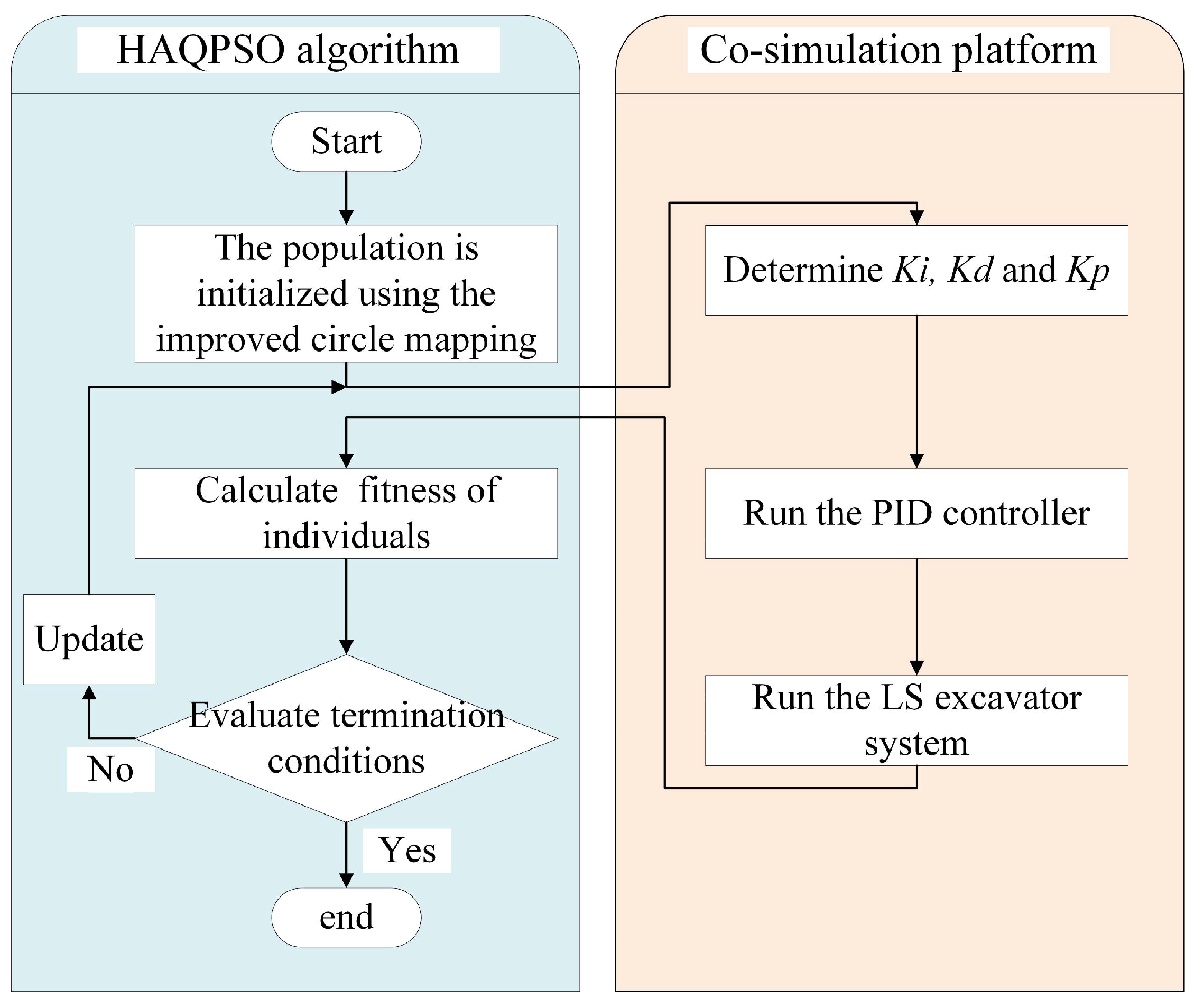
4. HAQPSO-PID Controller Design

4.1. PID Controller

Hydraulic excavator system adopts PID controller to achieve trajectory control of actuators. Its standard form is:
{ u ( t ) = K p e ( t ) + K i 0 t e ( t ) d t + K d d e ( t ) d t e ( t ) = y ( t ) r ( t )
where e is the error between the desired trajectory r and the actual trajectory y, u is the control signal, and K p , K i and K d are the coefficients of the controller.
The PID controller adjusts PID parameters from control signal u based on the change in error e. Although the PID control structure is simple and widely used, the parameters of PID are difficult to adjust, which leads to poor control effects [23]. Therefore, the most critical aspect of the PID controller is the tuning of K p , K i and K d .

4.2. Quantum-Behaved Particle Swarm Optimization

Due to the simple computation, fast convergence, cheap implementation, and few control parameters, PSO has been widely used in optimization problems since its introduction [14,15]. However, the PSO algorithm is prone to premature convergence and cannot guarantee convergence to the optimal global solution. To better solve the above questions, Sun [24] studied the research results on particle convergence behavior of particles by Clerc et al. The QPSO was proposed by applying the idea of quantum motion to particle behavior, which is free from the limitation of the traditional velocity–position orbit model.
The fluctuation function is applied in QPSO to describe the state of particles so that the moving particles have wave properties and the search is more continuous. In addition, the Schrödinger equation is used to obtain the probability density function of each individual at any position, and the position equation of particles in the problem space is gained by introducing the Monte Carlo simulation. In the iterative search process, the divergence of particles is constrained by the attractor of the best position center in the current iteration, which improves the probability of particles’ appearance in the problem space. The global search capabilities of population can be considerably improved by tracking the individual best and global optimal to update the solution. Thus, the QPSO method outperforms the PSO algorithm in terms of global search performance.
In the standard QPSO algorithm, the position update rule of each particle is:
X i j ( t + 1 ) = p i j ( t ) ± α | m b e s t j ( t ) X i j ( t ) | ln ( 1 u )
where X is the location of particle, i ( i = 1 , 2 , 3 , M ) is the number of particles, j is the particle dimension, t is the number of iterations, u = rand ( 0 , 1 ) , and p i j ( t ) is the random location of particle i between the local optimal position and the global optimal position after t iterations. It is defined as:
p i j ( t ) = φ P b e s t i j ( t ) + ( 1 φ ) G b e s t j ( t )
where φ = rand ( 0 , 1 ) , P b e s t is the local optimal position of particles, and G b e s t is the global optimal position of particles. The corresponding update rules are:
P b e s t i j ( t ) = { X i j ( t ) f [ X i j ( t ) ] < f [ P b e s t i j ( t 1 ) ] P b e s t i j ( t 1 ) o t h e r s G b e s t i j ( t ) = { P b e s t i j f [ P b e s t i j ( t ) ] < f [ G b e s t j ( t 1 ) ] G b e s t j ( t 1 ) o t h e r s
where f is the fitness function.
α is the contraction–expansion coefficient (CE), and it is:
α = 0.5 + 0.5 × t max t t max
where t max is the maximum number of iterations.
m b e s t is the global optimal average local optimal position of the particles, and it is defined as:
m b e s t = 1 M i = 1 M P b e s t i j ( t )

4.3. Hybrid Adaptive Quantum-Behaved Particle Swarm Optimization

Although the standard QPSO has many advantages, it still has some shortcomings. The valve selection method and range of parameters of CE have a great influence on the algorithm performance. It was proved that α < 1.781 can make the particles converge reliably [25]. As the complexity of the problem increases, it may still enter into local convergence prematurely. Moreover, the position of the initial population is generated randomly, which has an impact on operation efficiency.
The parameters of the PID controller are tuned based on QPSO, and its tuning algorithm should have high efficiency. Therefore, the initial population, search range, and calculation methods of m b e s t , φ , and CE with HAQPSO are optimized in this paper, and HAQPSO is established to overcome the shortcomings of QPSO. The specific improvements are as follows.
(1)
Improve search range
To improve the operation efficiency of HAQPSO, the Ziegler–Nichols (Z-N) method is used to calculate the initial PID value, and the search range of PID parameters is selected near the initial values. The initial position of particles is randomly generated within the search range.
(2)
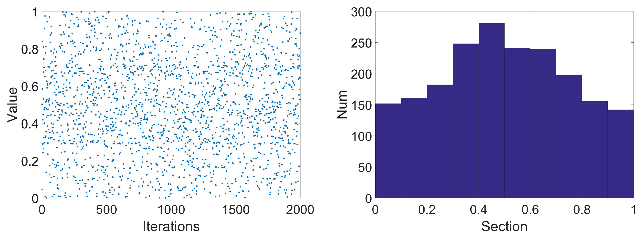
Initialized population optimization based on improved circle chaotic mapping
Since the particles are randomly generated in the initialization stage, it leads to the problem that the initial solutions are prone to aggregation, poor coverage in the solution space, and low variability among individuals. In contrast, chaotic is defined as mathematical randomness produced by simple deterministic systems, and has ergodicity and semi stochastic properties, depending on initial conditions [26]. Relevant experimental research shows that chaotic mapping is more useful than using random numbers in optimization problems [27]. Therefore, chaotic mapping is applied in the QPSO algorithm to optimize the initial population, ensure its distribution uniformity and diversity, and improve the quality and accuracy of the initial solution.
Circle mapping, an excellent mapping function, is applied to QPSO to improve its global optimization performance. However, circle mapping is still unevenly distributed [28]. The original circle chaotic mapping expression is:
c i + 1 = mod ( c i + b ( a 2 π ) sin ( 2 π c i ) , 1 )
where a and b are circle mapping parameters, generally a = 0.5 and b = 0.2 . When i = 2000 , the initial solution dimension distribution and histogram of initial solution dimension distribution are shown in Figure 5.
It can be seen from Figure 5 that the circle mapping is still unevenly distributed, with dense values between [0.4, 0.7]. Hence, the circle mapping formula has been improved to ensure the chaotic values are more uniformly distributed. The improved circle chaotic mapping expression is:
c i + 1 = mod ( c i + b ( a π ) sin ( π c i ) cos ( π c i ) + rand ( 0 , 1 ) , 1 )
The improved initial distribution diagram and initial solution dimension distribution histogram are shown in Figure 6. Compared with the original circle chaotic mapping, the improved circle has a more uniform search range between [0–1] and the distribution is more uniform. Therefore, the improved circle mapping is used to initialize the population to enhance its diversity, which in turn improves the optimization ability of QPSO.
The improved circle chaotic mapping is introduced in QPSO, and the initial particle population is:
x i j = c i ( u b l b ) + l b
where u b and l b are the upper and lower bounds of the search space, respectively.
(3)
Gaussian distribution variational operator
Gaussian distribution is the most widely used of the continuous probability distributions. To advance the searching ability of QPSO, the mutation operation is increased in the optimization process. When the population falls into the local optimum, a disturbance is added to improve the global search performance. It is given by:
m j ( t ) = m b e s t + ε ϕ
where ε is a predetermined parameter, which is set to ε = 0.001 in this paper, and ϕ is a Gaussian random distribution with a mean of 0 and a variance of 1. Equation (22) becomes:
X i j ( t + 1 ) = p i j ( t ) ± α | m j ( t ) X i j ( t ) | ln ( 1 u )
The mutation of the particle swarm decreases with the iteration of generations. It is applied to all particles at the beginning of the search to increase the search range of particles. During the middle of the search, it is applied to some particles for improving the convergence speed of the algorithm. At the end of the search, there is no more mutation, enabling the particles to perform a fine search in the vicinity of the optimal solution. Setting different mutation particles in different searching periods can effectively enhance the global search ability and searching speed of particles. Figure 7 shows the Gaussian mutation operation process when the number of iterations is 100.
(4)
Adaptive weight φ
Analyzing the QPSO update mode, the optimal location of individual is mostly determined by φ . The global optimum and the individual optimum must be effectively balanced in order to achieve better optimization performance. However, the traditional QPSO is generated randomly and cannot guarantee the search for the global optimum. Therefore, the random weight is converted to dynamic weight in the iterative process. The adaptive weight φ is defined as:
φ = exp ( f ( j ) / m ) ( 1 + exp ( f ( j ) / m ) ) i t e r
where φ is the average fitness value and f ( j ) is the fitness value.
(5)
Dynamic adjustment of CE
As the only control parameter that needs to be set manually, the control strategy of CE has a substantial impact on the performance of algorithm. CE decreases linearly with the increase of iterations in QPSO, which reduces the convergence speed and accuracy of the algorithm. However, the linear drop of CE in the early stages of particle search easily falls into the local ideal, whereas the linear decline of CE in the late stages of particle search may miss the optimal solution. CE should be dynamically changing during the search process. The adjustment function of CE is:
α = 1 1 + e 20 ( i t e r / m a x g e n 0.7 )
When the number of iterations is 100, the curves of CE in QPSO and HAQPSO are shown in Figure 8.
Finally, the HAQPSO algorithm is obtained as shown below.
Algorithm HAQPSO Algorithm
1: Initialization: population size, maximum iteration number.
2: Determine the initial particle population according to Equation (29).
3: While current number of iterations is less than the maximum number of iterations,
4: Calculate the fitness value of each particle according to Equation (34);
5: Calculate Pbest for each particle and Gbest for the swarm;
6: Calculate best position m b e s t according to Equation (26);
7: Calculate φ   and p i j according to Equations (23) and (32);
8: Calculate α   and   m j ( t ) according to Equations (30) and (33);
9: Update the position for each particle according to Equation (31);
10: Current number of iterations = current number of iterations + 1;
11: Output: Optimum PID parameters.

4.4. PID Parameter Tuning Based on HAQPSO

The purpose of the HAQPSO algorithm is to search the optimal PID gains for meeting the requirements of precise trajectory control for compound excavator operations. Every particle representing K p , K i and K d files through a three-dimensional search space to seek the optimal position by the HAQPSO algorithm. In the process of optimization, the convergence of the algorithm to the global optimal solution is determined by the objective function. Commonly used objective functions include integral squared error (ISE), integral absolute error (IAE) and time integral and absolute error (ITAE) [14,15,28]. In order to obtain good transient response and minimum steady-state error of the controlled object, the minimum value of ITAE is the objective function. Meanwhile, the objective function adds the square of the input control signal to avoid excessive control. The parameters of the PID controller are optimized online by the HAQPSO algorithm to realize the precise control for the multi-actuator compound trajectory of LS hydraulic excavator. The fitness function f and the objective function J can be written as:
f = 1 / J = 0 ( ω 1 | e ( t ) | + ω 2 u 2 ( t ) ) d t
where e ( t ) is the error value between the expected trajectory and the actual trajectory, u ( t ) is the controller output, and ω 1 and ω 2 are the corresponding weights.
The flow of HAQPSO tuning PID parameters is shown in Figure 9.

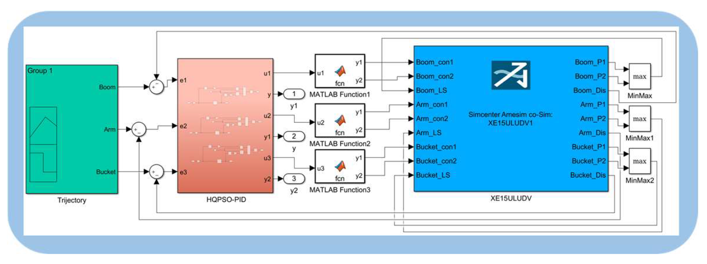
5. Hydraulic Excavator Co-simulation Platform

Controller performance tests performed directly on excavator are generally time-consuming, labor-intensive and dangerous. Therefore, a simulation model of the LS excavator is established, and the performance of the HAQPSO algorithm to optimize the PID controller in multi-actuator compound trajectory control of the LS hydraulic excavator is tested online. An electrohydraulic co-simulation platform of the LS excavator is constructed, as shown in Figure 10 and Figure 11. The platform is built according to the mechanical structure and hydraulic principles of the excavator, which can effectively reflect some nonlinear factors in the hydraulic system. Many studies have demonstrated the effectiveness and reliability of combined simulation in studying the performance of construction machinery [29,30,31].
The LS excavator model is built in AMESIM. The hydraulic system consists of a hydraulic component design (HCD) library and hydraulic components established according to parameters, including the LS pump, multiway valve, shuttle valve, hydraulic cylinder, oil tank, oil pipe, etc. The mechanical system is built by the mechanical library, which is based on mapping the actual mass, size, and moment of inertia of each actuator. The control strategy is constructed in Matlab/Simulink through co-simulation control. The box section is the interface between AMEsim and Matlab/Simulink. Table 1 lists the main parameters in the platform.

6. Experiment Results and Discussion

6.1. Performance Analysis of HAQPSO Performance

To verify the performance of the HAQPSO algorithm, the experiments are performed using four classical benchmark functions. These benchmark functions are widely used in numerical optimization algorithms [32,33,34], where Sphere and Rosenbrock are the unimodal functions and Rastrigin and Ackley are multimodal functions. The settings of the functional form, search range, and initialization range of the benchmark functions are shown in Table 2. n denotes the dimension of the solution space. The compared optimization algorithms are PSO, QPSO, and HAQPSO.
For all compared algorithms, experiments are conducted with particle populations N of 20, 50, and 80, particle dimensions D of 10, 30, and 50, and maximum iterations T of 1000, 1500, and 2000, respectively. Each case is run 100 times separately and the average value of the optimal solution is calculated to test the difference between the algorithms’ solution accuracy and stability. The convergence criterion is set to the maximum number of iterations. All experiments are performed using MATLAB 2016b on a personal computer with an Intel Core i7-9700F 3.0 GHz CPU with 16 GB memory. The final results of each benchmark function are shown in Table 3, Table 4, Table 5 and Table 6.
As seen from Table 3, Table 4, Table 5 and Table 6, for unimodal functions, the HAQPSO achieves better results than PSO and QPSO. The QPSO results are generally better than PSO, though in the Rosenbrock function, QPSO results are inferior to PSO at 50 particles. When the number of particles is fixed, the results of PSO, QPSO, and HAQPSO all increase with increases in dimension and iteration number. When the dimension and iteration number are determined, the algorithm results decrease with the increase in particle numbers. The two unimodal functions show the same pattern. For multimodal functions, the results of HAQPSO still outperformed those of PSO and QPSO for different particle numbers, different dimensions and different iterations, and both multimodal functions show the same variation pattern as the unimodal functions. Through the above analysis, it is demonstrated that the proposed HAQPSO algorithm outperforms PSO and QSPO in terms of optimization ability.
To vividly illustrate the performance advantages of HAQPSO, the convergence processes of the average fitness values for the four functions are shown in Figure 12, Figure 13, Figure 14 and Figure 15. It can be seen in Figure 12 that the optimal result of HAQPSO algorithm is better than QPSO and PSO. However, the convergence speed of HAQPSO and QPSO is lower than PSO in the early stage. With the increase in iteration numbers, the QPSO and HAQPSO algorithms converge faster than PSO. Both algorithms can produce better solutions in the final stage of searching, and the results of HAQPSO algorithm are better. Therefore, HAQPSO is more advantageous than QPSO. In Figure 13, the same pattern is observed in the Rosenbrock function test: HAQPSO is superior to QPSO and PSO in the optimal results. In addition, the initial solution of HAQPSO is significantly better than PSO and QPSO. This shows that the added circle mapping proposed can optimize the range of initial solutions.
In Figure 14, the optimal result of HAQPSO is also best in Rastrigin function, but the effect is not obvious. However, HAQPSO has the smallest number of iterations to search for the optimal solution. The optimal results of HAQPSO are also obviously better than QPSO and PSO in Figure 15. As with the Sphere function, the initial iteration speed of QPSO and HAPQSO is not as fast as that of PSO, but in the middle and late stages, HAQPSO is able to produce more optimal solutions. This indicates that HAQPSO does not fall into local convergence, and the particles enter a small area of fine search with better convergence accuracy than PSO and QPSO under the effect of adaptive learning. It is further verified that HAQPSO has better search accuracy and global convergence than PSO and QPSO.

6.2. Simulation Model Validation

The accuracy of the above co-simulation platform is verified by an LS hydraulic excavator, as shown in Figure 16. The joystick angle (Figure 17) is utilized as the input signal, and the same data as in the experiment are used. The experiment is a complete extension–retraction action of the bucket. Figure 18 shows the simulation results and the actual results. It can be seen that the co-simulation platform can effectively simulate the excavator actuator action. Therefore, in order to improve the efficiency, the co-simulation platform can effectively evaluate the performance of different controllers in controlling the excavator multiple actuators’ compound trajectory.

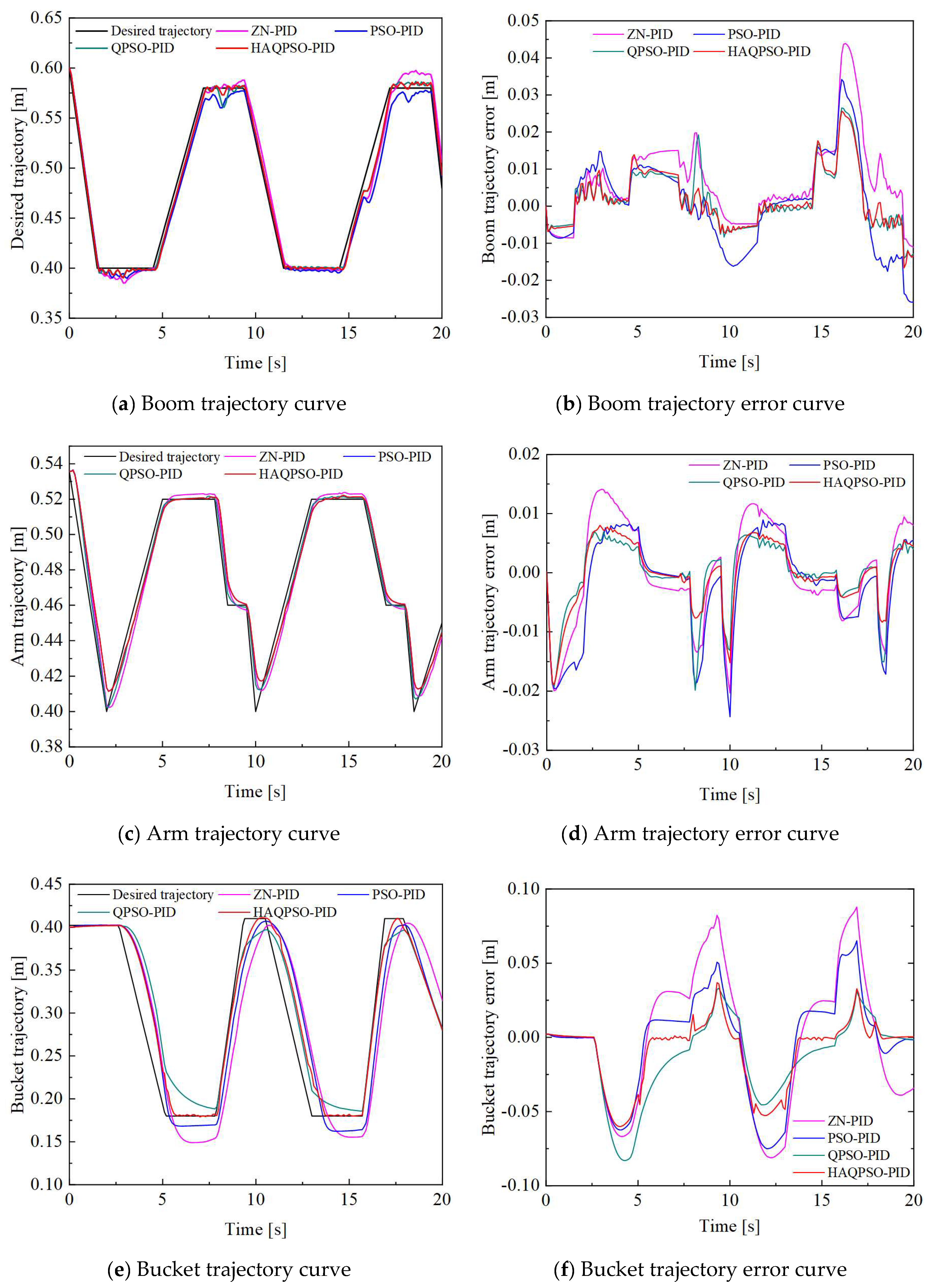
6.3. Trajectory Control Experiment

During excavator operation, the most frequent action is the actuator compound operation, which completes the excavator descending, internal retraction, ascending, and external swing operation cycle. To verify the performance of the proposed HAQPSO-PID controller in excavator dynamic trajectory, comparative experiments are carried out with different approaches: HAQPSO-PID, ZN-PID, PSO-PID, and QPSO-PID. The desired trajectory signals of boom, arm, and bucket are also provided, and their desired trajectories are used as position inputs to evaluate the efficacy of different excavator trajectory control methods. Table 7 shows the parameter-tuning results of the ZN-PID controller.
The main operating parameters that need to be determined in QPSO include population size, the number of iterations, and the range of search. To the best of our knowledge, there is no mature theory to choose reasonable values for these parameters [35], but ranges have been studied in some research [34,36,37,38]. According to the results of the literature discussion, the parameters of PSO-PID, QPSO-PID, and HAQPSO-PID are established as shown in Table 8.
The trajectory and trajectory error curves of boom, arm and bucket are shown in Figure 19, and it can be seen that HAQPSO-PID and ZN-PID, PSO-PID and QPSO-PID have certain control effects on the trajectories of multiple actuators. However, the maximum error of all trajectories occurs in the actuator reversing stage due to the sudden change in pressure and flow. Meanwhile, the trajectory control precision interferes with others due to the mutual coupling of the three actuators. The trajectory error of HAQPSO-PID is better than the other three approaches for boom, arm and bucket, as shown in Figure 20. Taking boom as an example, the trajectory error range of HAQPSO-PID is only 0.0403 m, which is smaller than the 0.0601 m of ZN-PID, 0.0549 m of PSO-PID, and 0.0445 m of QPSO-PID, and the error accuracy is improved by 32.95%, 26.59% and 9.44%, respectively. Therefore, HAPSO-PID has the highest control accuracy in terms of the trajectory error curve.
Figure 20 shows the iteration curves of HAQPSO-PID, QPSO-PID and PSO-PID controllers for the boom, arm and bucket trajectories after 100 iterations. Table 9 shows the corresponding optimal J, number of iterations, and rectified PID parameters. Figure 20 and Table 9 shows that the best J and iteration number of HAQPSO-PID are smaller than those of PSO-PID and QPSO-PID. Taking the boom as an example, HAQPSO-PID can be converged after 27 generations with an optimal fitness value of 22.1850, while PSO-PID needs 62 generations to complete convergence, and the optimal fitness value is 21.9931. QPSO-PID needs 43 generations, with a best-fit value of 21.9931. In summary, the comparative analysis verifies that the HAQPSO-PID controller proposed in this paper has the best performance.
To further prove the excavator trajectory control accuracy of the HAQPSO-PID controller, the root mean square error (RMSE) of the bucket, arm, and boom trajectory is calculated, as shown in Table 10. The results show that among the four different PID controllers, the RMSE of HAQPSO-PID is the smallest, which indicates that HAQPSO-PID has good trajectory control performance and further verifies the effectiveness of the HAQPSO-PID method proposed in this paper.
From what has been discussed above, the control accuracy, convergence speed, and other indicators are improved in the trajectory control of the excavator using the proposed HAQPSO-PID controller. The effectiveness of this method is verified.

7. Conclusions

In this research, an HAQPSO-PID controller is proposed to improve the accuracy of multi-actuator compound trajectory control of LS hydraulic excavator. The HAQPSO combines QPSO with circle chaotic mapping, Gaussian mutation operators, and adaptive adjustment to avoid premature convergence in the basic QPSO algorithm. The results show that the proposed HAQPSO algorithm can better tune the PID controller. Considering the nonlinear relationship in the excavator hydraulic system, the LS hydraulic excavator model with pump control subsystem and valve control subsystem is established. Combined with the parameters measured by the real excavator, a co-simulation platform is constructed. The accuracy of the co-simulation platform is verified through comparing experiments and simulations.
The trajectory control experiments of boom, arm, and bucket are carried out based on the co-simulation platform. Comparative analysis results for the trajectory error curve, trajectory error range, number of iterations, and RMSE show that HAQPSO-PID has higher control accuracy and faster convergence than other control methods. The accuracy of the excavator trajectory control can be effectively improved. The effectiveness of the HAQPSO algorithm in setting PID controller parameters in excavator nonlinear system position control is revealed. On the premise of ensuring the accurate control of excavator trajectory, how to reduce its energy consumption will be a future research direction.

Author Contributions

Conceptualization, H.S. and G.L.; methodology, H.S. and X.X.; data curation, Z.L. All authors have read and agreed to the published version of the manuscript.

Funding

This research was funded by the National Key Research and Development Program of China, (Grant No.2020YFB1709902).

Institutional Review Board Statement

Not applicable.

Informed Consent Statement

Not applicable.

Data Availability Statement

Not applicable.

Acknowledgments

The authors would like to thank Qiang Qin, Yubing Xu, and others of XCMG Excavator Machinery Business Department for their help in this research, and express sincere appreciation to the reviewers of this paper for their helpful comments.

Conflicts of Interest

The authors declare no conflict of interest.

References

  1. Do, T.C.; Dang, T.D.; Dinh, T.Q.; Ahn, K.K. Developments in energy regeneration technologies for hydraulic excavators: A review. Renew. Sustain. Energy Rev. 2021, 145, 111076. [Google Scholar] [CrossRef]
  2. Reginald, N.; Seo, J.; Cha, M. Integrative Tracking Control Strategy for Robotic Excavation. Int. J. Control Autom. Syst. 2021, 19, 3435–3450. [Google Scholar] [CrossRef]
  3. Chen, C.; Zhu, Z.; Hammad, A. Automated excavators activity recognition and productivity analysis from construction site surveillance videos. Autom. Constr. 2020, 110, 103045. [Google Scholar] [CrossRef]
  4. Lee, C.S.; Bae, J.; Hong, D. Contour control for leveling work with robotic excavator. Int. J. Precis. Eng. Manuf. 2013, 14, 2055–2060. [Google Scholar] [CrossRef]
  5. Shen, W.; Wang, J. Adaptive Fuzzy Sliding Mode Control Based on Pi-sigma Fuzzy Neutral Network for Hydraulic Hybrid Control System Using New Hydraulic Transformer. Int. J. Control Autom. Syst. 2019, 17, 1708–1716. [Google Scholar] [CrossRef]
  6. Zabihifar, S.H.; Yushchenko, A.S.; Navvabi, H. Robust control based on adaptive neural network for Rotary inverted pendulum with oscillation compensation. Neural Comput. Appl. 2020, 32, 14667–14679. [Google Scholar] [CrossRef]
  7. Kim, J.; Jin, M.; Choi, W.; Lee, J. Discrete time delay control for hydraulic excavator motion control with terminal sliding mode control. Mechatronics 2019, 60, 15–25. [Google Scholar] [CrossRef]
  8. Dao, H.V.; Na, S.; Nguyen, D.G.; Ahn, K.K. High accuracy contouring control of an excavator for surface flattening tasks based on extended state observer and task coordinate frame approach. Autom. Constr. 2021, 130, 103845. [Google Scholar] [CrossRef]
  9. Park, J.; Cho, D.; Kim, S.; Kim, Y.B.; Kim, P.Y.; Kim, H.J. Utilizing online learning based on echo-state networks for the control of a hydraulic excavator. Mechatronics 2014, 24, 986–1000. [Google Scholar] [CrossRef]
  10. Hua, H.; Fang, Y.; Zhang, X.; Qian, C. Auto-tuning nonlinear PID-type controller for rotorcraft-based aggressive transportation. Mech. Syst. Signal Process. 2020, 145, 106858. [Google Scholar] [CrossRef]
  11. Lui, D.G.; Petrillo, A.; Santini, S. An optimal distributed PID-like control for the output containment and leader-following of heterogeneous high-order multi-agent systems. Inf. Sci. 2020, 541, 166–184. [Google Scholar] [CrossRef]
  12. Zhang, S.; Minav, T.; Pietola, M.; Kauranne, H.; Kajaste, J. The effects of control methods on energy efficiency and position tracking of an electro-hydraulic excavator equipped with zonal hydraulics. Autom. Constr. 2019, 100, 129–144. [Google Scholar] [CrossRef]
  13. Do, T.C.; Tran, D.T.; Dinh, T.Q.; Ahn, K.K. Tracking Control for an Electro-Hydraulic Rotary Actuator Using Fractional Order Fuzzy PID Controller. Electronics 2020, 9, 926. [Google Scholar] [CrossRef]
  14. Ye, Y.; Yin, C.-B.; Gong, Y.; Zhou, J.-J. Position control of nonlinear hydraulic system using an improved PSO based PID controller. Mech. Syst. Signal Process. 2017, 83, 241–259. [Google Scholar] [CrossRef]
  15. Feng, H.; Ma, W.; Yin, C.; Cao, D. Trajectory control of electro-hydraulic position servo system using improved PSO-PID controller. Autom. Constr. 2021, 127, 103722. [Google Scholar] [CrossRef]
  16. Zhang, H.; Li, L.; Zhao, J.; Zhao, J. The hybrid force/position anti-disturbance control strategy for robot abrasive belt grinding of aviation blade base on fuzzy PID control. Int. J. Adv. Manuf. Technol. 2021, 114, 3645–3656. [Google Scholar] [CrossRef]
  17. Cao, F. PID controller optimized by genetic algorithm for direct-drive servo system. Neural Comput. Appl. 2018, 32, 23–30. [Google Scholar] [CrossRef]
  18. Zhang, C.; Ding, S. A stochastic configuration network based on chaotic sparrow search algorithm. Knowl. Based Syst. 2021, 220, 106924. [Google Scholar] [CrossRef]
  19. Abualigah, L.; Yousri, D.; Abd Elaziz, M.; Ewees, A.A.; Al-qaness, M.A.A.; Gandomi, A.H. Aquila Optimizer: A novel meta-heuristic optimization algorithm. Comput. Ind. Eng. 2021, 157, 107250. [Google Scholar] [CrossRef]
  20. Van den Bergh, F. An Analysis of Particle Swarm Optimizers. Ph.D. Thesis, University of Pretoria, Pretoria, South Africa, 2001. [Google Scholar]
  21. Shi, Y.; Li, W.; Lu, P.; Chen, F.; Qi, X.; Xiong, C. Research on hydraulic motor control system based on fuzzy neural network combing sliding mode control and time delay estimation. J. Intell. Fuzzy Syst. 2022, 43, 3815–3826. [Google Scholar] [CrossRef]
  22. Fu, S.; Wang, L.; Lin, T. Control of electric drive powertrain based on variable speed control in construction machinery. Autom. Constr. 2020, 119, 103281. [Google Scholar] [CrossRef]
  23. Nie, Z.Y.; Zhu, C.; Wang, Q.G.; Gao, Z.; Shao, H.; Luo, J.L. Design, analysis and application of a new disturbance rejection PID for uncertain systems. ISA Trans. 2020, 101, 281–294. [Google Scholar] [CrossRef] [PubMed]
  24. Sun, J.; Xu, W.B.; Feng, B. A global search strategy of quantum-behaved particle swarm optimization. In Proceedings of the 2004 IEEE Conference of Cybernetics and Intelligent Systems, Singapore, 1–3 December 2004. [Google Scholar]
  25. Sun, J.; Fang, W.; Wu, X.J.; Palade, V.; Xu, W.B. Quantum-Behaved Particle Swarm Optimization: Analysis of Individual Particle Behavior and Parameter Selection. Evol. Comput. 2012, 20, 349–393. [Google Scholar] [CrossRef] [PubMed]
  26. Varol Altay, E.; Alatas, B. Bird swarm algorithms with chaotic mapping. Artif. Intell. Rev. 2019, 53, 1373–1414. [Google Scholar] [CrossRef]
  27. Caponetto, R.; Fortuna, L.; Fazzino, S.; Xibilia, M.G. Chaotic sequences to improve the performance of evolutionary algorithms. IEEE Trans. Evol. Comput. 2003, 7, 289–304. [Google Scholar] [CrossRef]
  28. Arora, S.; Anand, P. Chaotic grasshopper optimization algorithm for global optimization. Neural Comput. Appl. 2018, 31, 4385–4405. [Google Scholar] [CrossRef]
  29. Xing, H.-Y.; Zhao, J.-Y.; Yin, X.; Ding, H.-G.; Meng, X.-Z.; Li, J.-S.; Wang, G.-Y. Simulated research on large-excavator boom based on hydraulic energy recovery. Proc. Inst. Mech. Eng. Part C J. Mech. Eng. Sci. 2021, 236, 10690–10700. [Google Scholar] [CrossRef]
  30. He, C.; Wang, J.; Wang, R.; Zhang, X. Research on the characteristics of hydraulic wind turbine with multi-accumulator. Renew. Energy 2021, 168, 1177–1188. [Google Scholar] [CrossRef]
  31. Wang, H.P.; Mustafa, G.I.Y.; Tian, Y. Model-free fractional-order sliding mode control for an active vehicle suspension system. Adv. Eng. Softw. 2018, 115, 452–461. [Google Scholar] [CrossRef]
  32. Chen, K.; Zhou, F.; Liu, A. Chaotic dynamic weight particle swarm optimization for numerical function optimization. Knowl. Based Syst. 2018, 139, 23–40. [Google Scholar] [CrossRef]
  33. Yao, X.; Liu, Y.; Lin, G. Evolutionary Programming Made Faster. IEEE Trans. Evol. Comput. 1999, 3, 82–88. [Google Scholar]
  34. Chen, S. Quantum-Behaved Particle Swarm Optimization with Weighted Mean Personal Best Position and Adaptive Local Attractor. Information 2019, 10, 22. [Google Scholar] [CrossRef] [Green Version]
  35. Feng, H.; Yin, C.-B.; Weng, W.-W.; Ma, W.; Zhou, J.-J.; Jia, W.-H.; Zhang, Z.-L. Robotic excavator trajectory control using an improved GA based PID controller. Mech. Syst. Signal Process. 2018, 105, 153–168. [Google Scholar] [CrossRef]
  36. Coelho, L.S. Novel Gaussian quantum-behaved particle swarm optimiser applied to electromagnetic design. IET Sci. Meas. Technol. 2007, 1, 290–294. [Google Scholar] [CrossRef]
  37. Sun, J.; Wu, X.; Palade, V.; Fang, W.; Lai, C.-H.; Xu, W. Convergence analysis and improvements of quantum-behaved particle swarm optimization. Inf. Sci. 2012, 193, 81–103. [Google Scholar] [CrossRef]
  38. Tian, N.; Lai, C.-H. Parallel quantum-behaved particle swarm optimization. Int. J. Mach. Learn. Cybern. 2013, 5, 309–318. [Google Scholar] [CrossRef]
Figure 1. Hydraulic system diagram of the LS hydraulic excavator.
Machines 11 00010 g001
Figure 2. Control flowchart of the LS hydraulic excavator system.
Machines 11 00010 g002
Figure 3. Schematic diagram of the multiway valve. 1. Safety valve, 2. spool, 3. pressure compensation valve, 4. load check valve.
Machines 11 00010 g003
Figure 4. Schematic diagram of the LS pump.
Machines 11 00010 g004
Figure 5. Distribution diagram and distribution histogram of circle mapping.
Machines 11 00010 g005
Figure 6. Distribution diagram and distribution histogram of improved circle mapping.
Machines 11 00010 g006
Figure 7. Gaussian mutation operation.
Machines 11 00010 g007
Figure 8. The comparison curves of CE in different methods.
Machines 11 00010 g008
Figure 9. Framework of HAQPSO tuning PID controller parameters.
Machines 11 00010 g009
Figure 10. Co-simulation platform of LS excavator.
Machines 11 00010 g010
Figure 11. Co-simulation platform of controller.
Machines 11 00010 g011
Figure 12. Convergence process of Sphere function (M = 20, D = 10, T = 1000).
Machines 11 00010 g012
Figure 13. Convergence process of Rosenbrock function (M = 80, D = 10, T = 1000).
Machines 11 00010 g013
Figure 14. Convergence process of Rastrigin function (M = 20, D = 10, T = 1000).
Machines 11 00010 g014
Figure 15. Convergence process of Ackley function (M = 50, D = 30, T = 1500).
Machines 11 00010 g015
Figure 16. Experimental platform of LS excavator.
Machines 11 00010 g016
Figure 17. Input signal of simulation model.
Machines 11 00010 g017
Figure 18. Comparison of trajectory between experiment and simulation.
Machines 11 00010 g018
Figure 19. Experimental results of actuators under compound operation.
Machines 11 00010 g019
Figure 20. Iteration curves of different tuning methods with different actuators. (a) Iteration curves of different tuning methods with boom, (b) Iteration curves of different tuning methods with arm, (c) Iteration curves of different tuning methods with bucket.
Machines 11 00010 g020aMachines 11 00010 g020b
Table 1. Basic parameters of the co-simulation platform.
ParameterValueUnit
Oil density850kg/m3
Oil bulk modulus17,000bar
Engine speed2300r/min
Pump maximum displacement34cc/rev
Pump volumetric efficiency0.92
Pump hydraulic–mechanical efficiency0.96
Relief valve cracking pressure270bar
Pressure compensation valve piston diameter10mm
Pressure compensation valve rod diameter5mm
Spring force at zero displacement37.8N
Spring rate20N/mm
Coefficient of pressure compensating valve viscous friction50N/m/s
Cylinder leakage coefficient0.01L/min/bar
Piston diameter of the boom hydraulic cylinder74mm
Rod diameter of boom hydraulic cylinder34mm
Travel of boom hydraulic cylinder650mm
Boom mass60.94kg
Moment of boom inertia1245.46kg/m2
Piston diameter of the arm hydraulic cylinder70mm
Rod diameter of arm hydraulic cylinder34mm
Travel of arm hydraulic cylinder503mm
Arm mass28.38kg
Moment of arm inertia127.57kg/m2
Piston diameter of the bucket hydraulic cylinder75mm
Rod diameter of bucket hydraulic cylinder34mm
Travel of bucket hydraulic cylinder410mm
Bucket mass16.55kg
Moment of Bucket inertia29.32kg/m2
Table 2. Classical high-dimension benchmark functions.
NameFunction ExpressionSearch DomainInitial Range
Sphere f 1 ( x ) = i = 1 n x i 2 [−100, 100]n[50, 100]
Rosenbrock f 3 ( x ) = i = 1 n 1 [ 100 ( x i + 1 x i 2 ) 2 + ( x i 1 ) 2 ] [−30, 30]n[15, 30]
Rastrigin f 4 ( x ) = i = 1 n ( x i 2 10 cos ( 2 π x i ) + 10 ) [−5.12, 5.12]n[2.56, 5.12]
Ackley f 5 ( x ) = 20 + e 20 e ( 1 5 1 n i = 1 n x i 2 ) e ( 1 n i = 1 n cos ( 2 π x i ) [−32, 32]n[16, 32]
Table 3. Test results of Sphere.
NDTAlgorithm
PSOQPSOHAQPSO
201010002.4332 × 10−63.2146 × 10−281.1313 × 10−43
3015009.8434 × 10−46.5730 × 10−177.047 × 10⁻¹⁷
5020005.9672 × 10−35.6147 × 10−51.6556 × 10−7
501010005.4372 × 10−104.4054 × 10−351.2969 × 10−60
3015002.7452 × 10−71.0317 × 10−232.0601 × 10−43
5020004.6132 × 10−41.9244 × 10−81.8286 × 10−19
801010001.2378 × 10−124.4054 × 10−461.5692 × 10−97
3015002.0232 × 10−42.1565 × 10−242.1925 × 10−52
5020008.4451 × 10−21.6424 × 10−111.8021 × 10⁻²⁵
Table 4. Test results of Rosenbrock.
NDTAlgorithm
PSOQPSOHAQPSO
2010100016.036615.48218.5116
30150046.207447.845837.3123
502000156.7582104.886082.8742
501010003.95655.14952.9243
30150036.632845.430723.2881
50200054.754149.978234.9334
801010003.90583.88842.5978
30150032.782345.915216.8176
50200047.909145.924428.0241
Table 5. Test results of Rastrigin.
NDTAlgorithm
PSOQPSOHAQPSO
201010008.62636.36945.1833
30150026.896722.325812.3823
50200041.414328.768522.2701
501010004.09923.72852.4873
30150031.325923.407322.3915
50200035.805524.872818.7974
801010003.23512.39791.9899
30150012.45368.69239.5942
50200025.627617.775316.3971
Table 6. Test results of Ackley.
NDTAlgorithm
PSOQPSOHAQPSO
201010005.6949 × 10−41.4460 × 10−144.4409 × 10⁻¹⁵
3015000.03690.00619.4508 × 10−8
5020000.09850.65912.8150 × 10−4
501010002.1999 × 10−61.5099 × 10−145.0804 × 10⁻¹⁵
3015000.00593.1556 × 10−71.9984 × 10⁻¹³
5020000.02540.00571.5727 × 10−9
801010008.1035 × 10−84.5409 × 10−154.4119 × 10⁻¹⁵
3015000.00169.3718 × 10−121.5099 × 10⁻¹⁴
5020000.00973.2142 × 10−51.4255 × 10⁻¹²
Table 7. Parameter optimization results by Z-N tuning method.
KpKiKd
Boom23.286.483.63
Arm21.965.372.17
Bucket19.645.892.48
Table 8. Parameters of PSO-PID, QPSO-PID and HAQPSO-PID.
ParameterPSO-PIDQPSO-PIDHAQPSO-PID
Population size303030
Maximum iteration number100100100
Search range of Kp[0, 40][0, 40]/
Search range of Ki[0, 10][0, 10]/
Search range of Kd[0, 10][0, 10]/
Learning coefficient 12//
Learning coefficient 22//
[Vmin Vmax][0, 0.9]//
Inertia weight0.6//
ω 1 0.9990.9990.999
ω 2 0.0010.0010.001
Table 9. Parameter optimization results by different tuning methods.
Tuning MethodIndicatorBoomArmBucket
PSO-PIDBest J22.1919.8426.13
Number of iterations625964
Kp21.0820.6323.09
Ki5.534.173.24
Kd3.733.964.35
QPSO-PIDBest J21.9919.6425.62
Number of iterations435165
Kp22.6121.5721.83
Ki4.626.755.79
Kd4.183.372.35
HQPSO-PIDBest J21.5119.3724.79
Number of iterations273857
Kp22.3419.9822.73
Ki6.978.344.52
Kd4.474.693.65
Table 10. Root mean square error of different methods.
MethodsRMSE
BoomArmBucket
ZN-PID12.945910.299944.9140
PSO-PID10.09779.654234.3970
QPSO-PID8.31537.764229.6588
HAQPSO-PID8.17986.644224.8488
Disclaimer/Publisher’s Note: The statements, opinions and data contained in all publications are solely those of the individual author(s) and contributor(s) and not of MDPI and/or the editor(s). MDPI and/or the editor(s) disclaim responsibility for any injury to people or property resulting from any ideas, methods, instructions or products referred to in the content.

