Article

Dynamic Modeling and Analysis of Loader Working Mechanism Considering Cooperative Motion with the Vehicle Body

1
School of Mechanical Engineering, University of Science and Technology Beijing, Beijing 100083, China
2
School of Mechanical and Automotive Engineering, Guangxi University of Science and Technology, Liuzhou 545006, China
*
Author to whom correspondence should be addressed.
These authors contributed equally to this work.
Machines 2023, 11(1), 9; https://doi.org/10.3390/machines11010009
Submission received: 15 November 2022 / Revised: 13 December 2022 / Accepted: 16 December 2022 / Published: 21 December 2022
(This article belongs to the Section Vehicle Engineering)

Abstract

:
Achieving precise load detection for Intelligent Loaders is an important task, which directly affects the operation energy efficiency and the fatigue life analysis for the loader’s working mechanism. The operation of the mechanism is regarded as a 3-DOF (degree of freedom) planar motion process coordinated with the vehicle body. Affected by complex dynamic coupling in motion, the existing dynamic models of the mechanism have the problem of insufficient accuracy, which is not conducive to the precise calculation of load. Taking the reverse six-linkage loader as the research object, an accurate dynamic model of the mechanism is established considering its cooperative motion with the vehicle body. Firstly, the kinematic description of the mechanism is given by the Rodriguez method. Then, to overcome the coupling effect caused by the cooperative motion, the sufficient inertia forces of the mechanism are established in joint space using the Lagrange method. Furthermore, to overcome the coupling effect caused by the complex structure, the Newton–Euler method is used to establish the force mapping relations between the joint space and the drive space by multi-body modeling. Finally, the dynamic model of the mechanism in drive space is obtained, and the specific mapping relations between the bucket force, the vehicle driving force, and the drive parameters are given. Compared with existing dynamic models in simulation, the analysis shows that the average and maximum absolute errors of the vehicle driving force calculated by the established model do not exceed 20% of the existing model errors, and the corresponding errors of the bucket force do not exceed 10% of the existing model errors, which proves that the motions of vehicle body and front-end mechanism, as well as the force of the tilt hydraulic cylinder, play important roles in improving the model accuracy. The established model is superior to existing models and is more suitable for cooperative motion with the vehicle body.

1. Introduction

Loaders are important construction machines whose primary task is to load and transport bulk materials such as rock and soil. They are widely used in different applications, such as mines, ports, and construction sites. The operation cycle of the loader is mainly divided into four stages: shoveling, transportation, unloading, and flattening, which are mainly completed by the loader’s working mechanism [1,2,3]. The operating load directly affects the performance of the working mechanism, so achieving precise load detection has been an important task realted to loaders [1,4].
The front-end mechanism of the loader is mainly a 2-DOF (degree of freedom) mechanism driven by a lift hydraulic cylinder and a tilt hydraulic cylinder. In practical application, the front-end mechanism and the vehicle body work together, that is, the motion of the front-end mechanism is usually accompanied by the forward or backward motion of the vehicle body. So, the operation of the loader’s working mechanism can be considered as a 3-DOF planar motion process driven by the vehicle body and the hydraulic cylinders [5]. The vehicle’s motion will bring additional inertia forces to the front-end mechanism, and the inertia forces of the front-end mechanism will affect the precise measurement of the operating load [6], etc. Therefore, building an accurate dynamic model of the working mechanism in the drive space has important theoretical and practical value for the research of the precise online detection for the load, the driving force distribution for the vehicle’s motion, etc.
A series of achievements have been made in the dynamic modeling of the loader’s working mechanism. The existing dynamic models can be roughly divided into the following three categories:
(1) Without considering the influence of the vehicle motion, the working mechanism is simplified as a dynamic model of the two-bar mechanism. Some scholars [5,7,8,9,10] have established dynamic models of the working mechanism, which was simplified as a two-bar mechanism when the vehicle body was static, for the research purpose of shoveling trajectory planning and control, load weight measurement, structural parameter optimization, etc. In the representative research [8], Kang et al. established a dynamic model of the reverse six-linkage mechanism, which was simplified as a two-bar mechanism (only boom and bucket) on the assumption that the load was balanced and the vehicle body was static, for measuring the load weight. Such models only considered the dynamic characteristics of the two bars (boom and bucket) in the joint space without considering the dynamic effects caused by the vehicle motion and neglected the tilt cylinder action (affected by the offset load) when converting to the drive space, resulting in a loss of accuracy.
(2) Without considering the influence of the vehicle motion, a simplified dynamic or static model of the working mechanism with dynamic compensation can be created. Some scholars [6,11,12,13,14,15,16,17,18,19,20,21,22,23] have established simplified dynamic or static models of the reverse six-linkage, TP-linkage, or agricultural working mechanisms that include dynamic compensation for some components or the offset load in the drive space. Such models are used in the research of shoveling trajectory planning, resistance analysis, load measurement, and structure optimization, etc. In the representative research [22], Madau et al. established a static model of the reverse six-linkage working mechanism with the dynamic compensation of the boom and then proposed an online estimation algorithm to calculate the load force. Such models only considered the dynamic characteristics of some components or the offset load in the drive space without considering the dynamic effects caused by the vehicle motion, resulting in insufficient accuracy in the cooperative motion with the vehicle body.
(3) Considering the influence of the vehicle motion, a static model of the working mechanism can be created. Some scholars [2,24,25] have established static models of the reverse six-linkage or TP-linkage working mechanisms in the drive space to study vehicle control, torque distribution, inertia parameter estimation, etc. In the representative research [2], Gao et al. established a static model of the reverse six-linkage working mechanism considering the load force and proposed a torque distribution strategy based on this model for vehicle driving control. Such models mainly calculated the driving force of the vehicle body to achieve the driving control for the loader without considering the dynamic effects caused by the motion of the front-end mechanism, resulting in insufficient accuracy in the cooperative motion with the front-end mechanism.
In a word, the above models have the problem of insufficient accuracy in the cooperative motion of the vehicle body and the front-end mechanism (i.e., the working mechanism works in a 3-DOF motion), which is not conducive to the load calculation and directly affects the operation energy efficiency and the fatigue life analysis of the mechanism system [4,26]. Therefore, achieving precise load detection puts forward higher accuracy requirements for the dynamic model of the working mechanism during operation.
To improve the accuracy of the dynamic model of the loader’s working mechanism during operation, an accurate dynamic model of the working mechanism is established in the 3-DOF motion, which fully considers the inertia forces and the coupling of the mechanism system, including the influence of the vehicle’s motion. Specifically, taking the reverse six-linkage loader as the research object, first, the kinematic description of the mechanism system in the joint space is given by the Rodriguez method, and then the kinematic model in the drive space is given by the motion mapping relations, which can provide basic motion state information for the dynamic modeling of the mechanism system. Then, drawing on the idea of analytical mechanics, considering the strong dynamic coupling characteristics of the mechanism system caused by the cooperative motion of the vehicle body and the front-end mechanism comprehensively, the displacement of the vehicle body is introduced as an independent generalized coordinate; thus, the inertia and generalized forces of the mechanism system, including the inertia forces caused by the vehicle motion, are fully established by the Lagrange method, and the dynamic model of the mechanism system is finally obtained in the joint space. Furthermore, drawing on the idea of vector mechanics and considering the structural coupling of the mechanism and the action of the tilt hydraulic cylinder mainly affected by the offset load, the Newton–Euler method is used to model the whole body and the single body of the mechanism system to find the force mapping relations between the joint space and the drive space. Finally, the dynamic model of the mechanism system is obtained in the drive space, and the specific mapping relations between the vehicle driving force, the bucket force and the drive space parameters are given. In the validation and analysis section, the simulation platform is first built, and then the kinematic model and the dynamic model are verified separately. In the dynamic model’s validation, by comparing it with the existing dynamic models, the analysis shows that the dynamic model built in this paper has higher accuracy and applies to the cooperative motion of the vehicle body and the front-end mechanism.

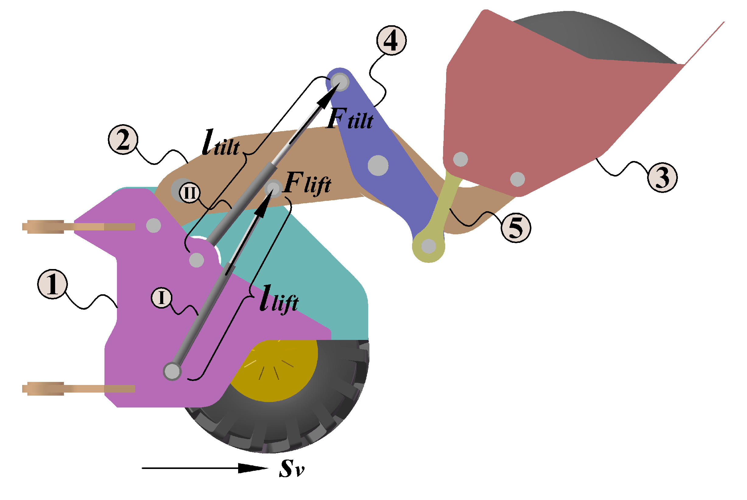
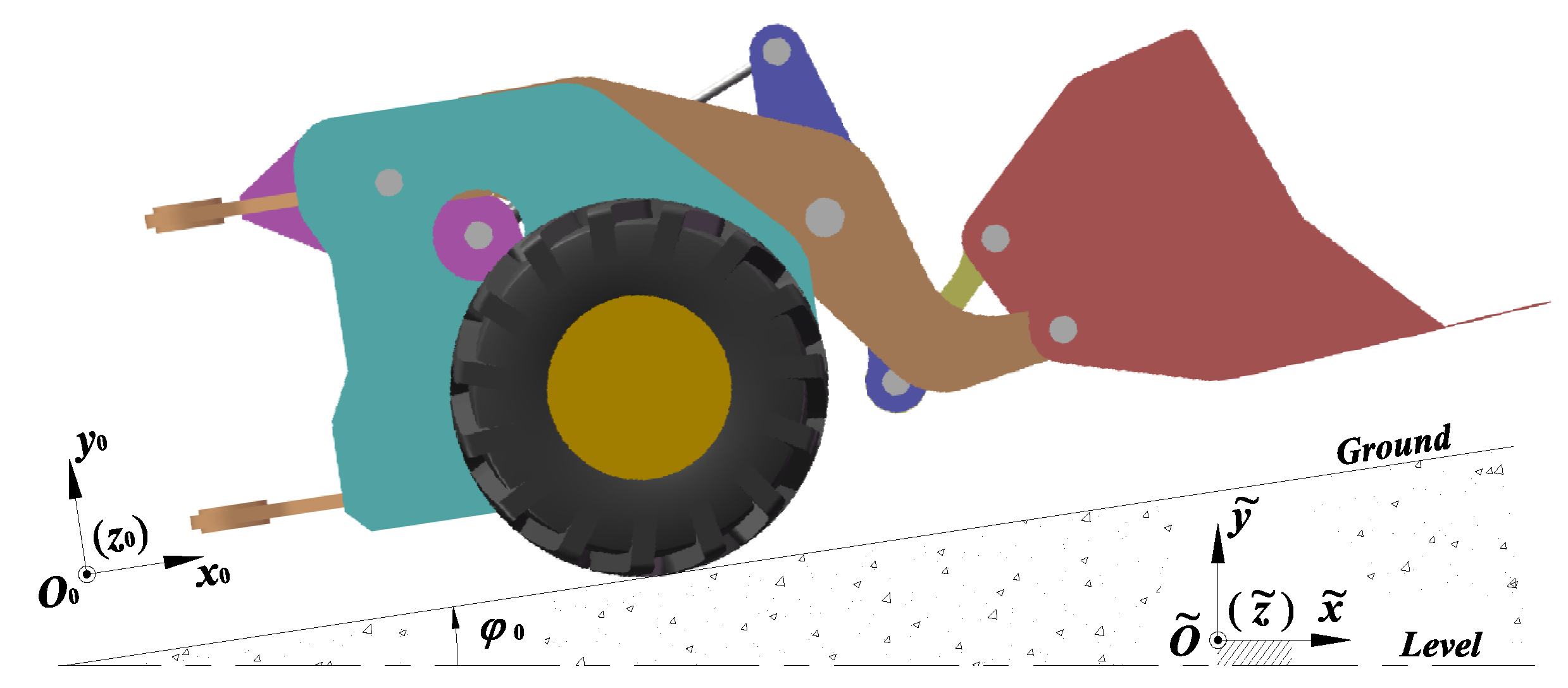
2. Drive Space and Parameters

In Figure 1, the working mechanism system of the reverse six-linkage loader can be considered to consist of five rigid bodies and two driving devices interconnected by revolute joints. Among them, bodies 1∼5 represent the vehicle body, boom, bucket, rotating bar, and connecting bar, respectively. Driving device I represents the lift hydraulic cylinder used to drive the boom up and down. Driving device II represents the tilt hydraulic cylinder used to drive the bucket’s rotation. The working surface (ground) of the loader is generally considered as a plane (not a level surface) during the shoveling operation of the working mechanism, and in this working condition, the motion of the vehicle body (body 1) is considered as a straight-line translation. As the mechanism system is 3-DOF when working, in practical application, the operators can realize the loader’s operation by driving the vehicle body and the hydraulic cylinder devices. In addition, the vehicle body’s velocity and the hydraulic cylinders’ lengths are easy and economical to observe. Therefore, the kinematic and dynamic models of the loader’s working mechanism built in the drive space have practical significance and value. The drive space can be described as follows:
R d r i v e 5 × 1 = s v ( t ) , l l i f t ( t ) , l t i l t ( t ) , F l i f t ( t ) , F t i l t ( t ) T
where t is the time variable, and the displacement s v ( t ) of the vehicle body, the length l l i f t ( t ) of the lift cylinder, the length l t i l t ( t ) of the tilt cylinder, the piston force F l i f t ( t ) of the lift cylinder, and the piston force F t i l t ( t ) of the tilt cylinder are considered as the drive space parameters. Here, the three independent variables, s v ( t ) , l l i f t ( t ) , and l t i l t ( t ) , are taken as the generalized coordinates in the drive space.
Due to the complex structural coupling of the working mechanism system, it is difficult to directly establish the kinematic and dynamic models in the drive space. Therefore, the kinematic and dynamic models can be established in the joint space first, and then the models can be established in the drive space by seeking the mapping relations between the joint space and the drive space.
(For comprehensive nomenclature of all the mathematical symbols used in the paper, see Abbreviations at the end of the text.)

3. Kinematic Description of Working Mechanism System

In this section, firstly, a kinematic model of the mechanism system considering vehicle motion is established in joint space, and then motion mapping relations between the joint space and drive space are given. Finally, the kinematic model of the mechanism system is obtained in drive space, which provides a basis for accurate dynamic modeling of the mechanism system.

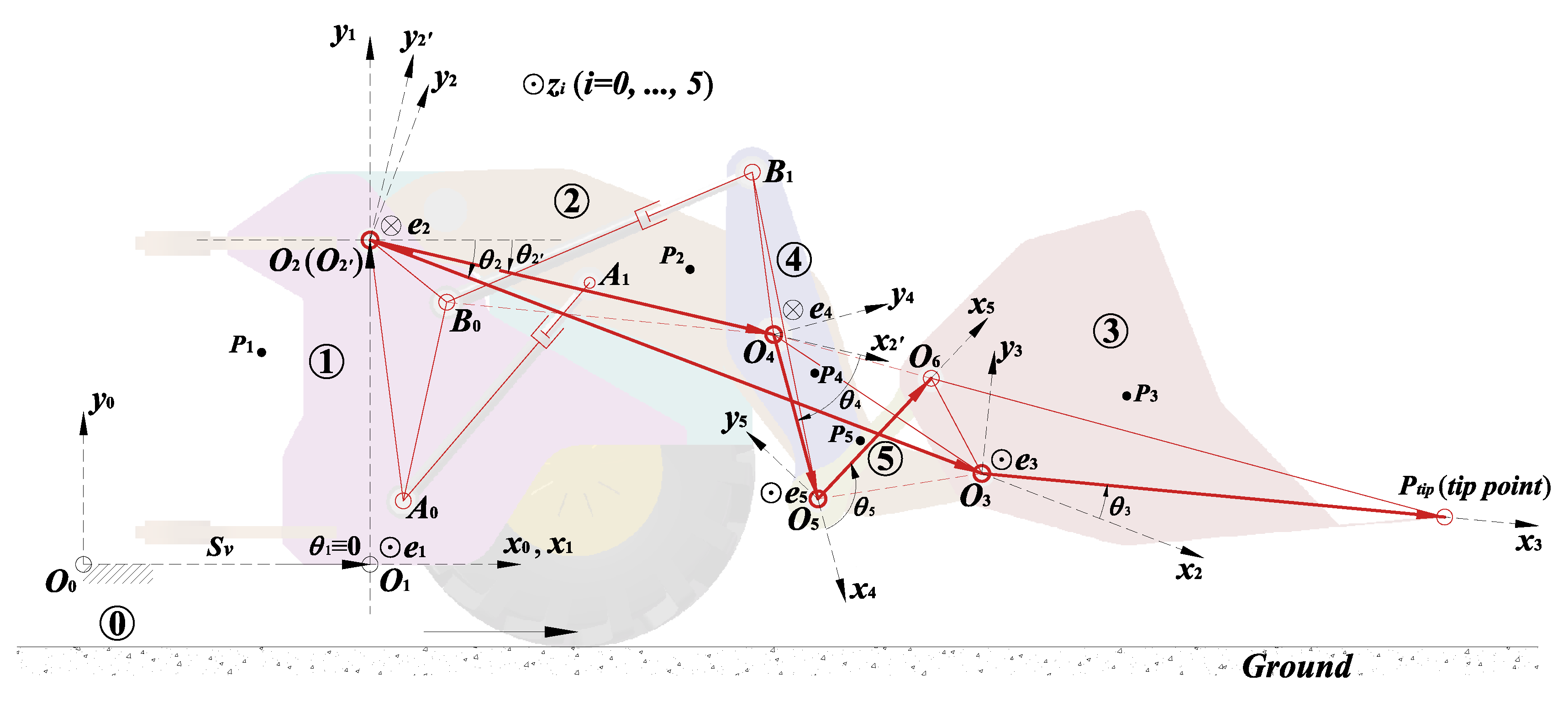
3.1. Kinematic Description in Joint Space

Based on the previous assumptions, in Figure 2, since the boom (body 2) and the bucket (body 3) of the loader are the most important working parts in the mechanism’s operation and the bucket tip P t i p is the key point, to facilitate the following dynamic modeling, the loader’s reverse six-linkage working mechanism system can be modeled as two parallel kinematic chains 1 and 2. Kinematic chain 1 is O 0 - O 1 - O 2 - O 3 - P t i p , and kinematic chain 2 is O 0 - O 1 - O 2 - O 4 - O 5 - O 6 . Without loss of generality, for each kinematic chain, the following kinematic descriptions can be given.
The motion of the loader with respect to the fixed reference frame (ground) O 0 x 0 y 0 z 0 is described by the joint coordinates s v and θ i i = 1 , , n . The coordinate s v (seen as a moving joint) represents the displacement of body 1. The coordinate θ i represents the relative rotation of the body i with respect to the body i-1 carried out about the joint axis determined by the unit vector e i . This vector is fixed to the body i-1. The point O i is placed on the direction e i and represents the center point of the i-th joint connecting the bodies i-1 and i. The local coordinate frames O i x i y i z i i = 1 , , n that are fixed to the bodies i = 1 , , n , respectively, are introduced (see Figure 2). As the local coordinate frame O 1 x 1 y 1 z 1 is considered a moving joint with respect to O 0 x 0 y 0 z 0 , here θ 1 0 , i s v = s v , 0 , 0 T i = 0 . Note that the left superscript i indicates that the components of the corresponding vectors and matrices are given in the O i x i y i z i local frame. The non-bold symbol corresponding to a vector in the following text represents the amplitude of the vector. Among them, l i j represents the length vector from point i to point j, and γ i j k represents the angle i j k .
Without loss of generality, it is assumed that the configuration θ i = 0 i = 1 , , n is a reference configuration of the loader and that, in this configuration, the axes of all local reference frames are parallel to the corresponding axes of the fixed reference frame, that is, x i x 0 , y i y 0 and z i z 0 . According to this, the transformation matrix R i , j i = 0 , , n ; j = 1 , , n from O j x j y j z j to O i x i y i z i reference frames have the form [27,28]:
R i , j = k = i + 1 j R k r = k = i + 1 j I + 1 cos θ k k e ˜ k 2 + k e ˜ k sin θ k , i < j
where R k r R 3 × 3 is the Rodriguez matrix [27], I R 3 × 3 is the identity matrix, and k e ˜ k R 3 × 3 is the skew-symmetric matrix [27,28] associated with the vector k e k . In addition, since the Rodriguez matrix is orthogonal [27], the following holds:
R i , j 1 = R i , j T R j , i = R i , j T
where the right superscript T denotes matrix transposition.
Now, in regard to the literature [28,29], the angular velocity ω i and the angular acceleration α i of the body i can be calculated recursively, respectively, as follows:
i ω i = R i 1 , i T i 1 ω i 1 + θ ˙ i i e i , i = 1 , , n
i α i = R i 1 , i T i 1 α i 1 + θ ¨ i i e i + θ ˙ i R i 1 , i T i 1 ω ˜ i 1 i 1 e i , i = 1 , , n
Based on the previous relations, the velocity v P i and the acceleration a P i of the any point P i of the body i, respectively, are given by the following recurrence relations (for proof, see ref. [29]):
i v P i = R i 1 , i T i 1 s ˙ v + i 1 v P i 1 , i = 1 i v P i = R i 1 , i T i 1 v P i 1 + i 1 ω ˜ i 1 i 1 l i 1 i 1 l P i 1 + i ω ˜ i i l P i , i = 2 , , n
i a P i = R i 1 , i T i 1 s ¨ v + i 1 a P i 1 , i = 1 i a P i = R i 1 , i T i 1 a P i 1 + i 1 α ˜ i 1 i 1 l i 1 i 1 l P i 1 + i α ˜ i i l P i + i ω ˜ i 2 i l P i + i 1 ω ˜ i 1 2 i 1 l i 1 i 1 l P i 1 , i = 2 , , n
where l i = l O i O i + 1 , l P i = l O i P i .
In Figure 2, it is obvious that the vectors e i i = 1 , , 5 have the following components:
i e i = i 1 e i = 0 , 0 , 1 T , i = 1 , 3 , 5 0 , 0 , 1 T , i = 2 , 4
Note that for body 0, 0 ω 0 = 0 , 0 , 0 T , 0 α 0 = 0 , 0 , 0 T , 0 v P 0 = 0 , 0 , 0 T , and 0 a P 0 = 0 , 0 , 0 T hold.
Therefore, for kinematic chain 1 i = 1 , 2 , 3 , the motion data of any point P i of the body i can be expressed by joint coordinates s v , θ 2 , θ 3 . Similarly, for kinematic chain 2 i = 1 , 2 , 4 , 5 , the motion data of any point P i of the body i can be expressed by joint coordinates s v , θ 2 , θ 4 , θ 5 . In fact, the front-end mechanism of the loader has 2-DOF. Considering the importance of kinematic chain 1 and facilitating the dynamic modeling, any joint angle can be expressed by selecting θ 2 , θ 3 as the generalized coordinates in the joint space. Specifically, θ 2 = θ 2 + γ O 3 O 2 O 4 , θ 4 and θ 5 can be expressed by θ 3 , either by the methods in the next section or in the literature [30]. For this, there is the motion mapping relation in the following form:
Θ j o i n t = Φ k 1 s v , θ 2 , θ 3 Θ j o i n t = s v , θ 2 , θ 2 , θ 3 , θ 4 , θ 5 T
In this section, the kinematic model of the mechanism is established in joint space, and the mapping relations between the motion data of any point P i and the joint coordinates s v , θ 2 , θ 3 are given.

3.2. Kinematic Description in Drive Space

Based on the explicit derivation method of the analytic geometry, this section establishes the motion mapping relations between joint space parameters θ 2 , θ 3 and drive space parameters l l i f t , l t i l t , so as to establish the kinematic model of the mechanism in the drive space. In Figure 2, when the design dimensions of each body are known, the motion mapping relations between the joint space and the drive space are derived as follows.
Mapping functions of the joint space parameter θ 2 :
γ A 0 O 2 A 1 = c o s 1 ( l O 2 A 0 2 + l O 2 A 1 2 l l i f t 2 / 2 l O 2 A 0 l O 2 A 1 ) γ ˙ A 0 O 2 A 1 = d γ A 0 O 2 A 1 d l l i f t l ˙ l i f t γ ¨ A 0 O 2 A 1 = d 2 γ A 0 O 2 A 1 d 2 l l f i t l ˙ l i f t 2 + d γ A 0 O 2 A 1 d l l i f t l ¨ l i f t
θ 2 = π / 2 γ A 0 O 2 y 1 + γ A 0 O 2 A 1 γ O 4 O 2 A 1 γ O 3 O 2 O 4 θ ˙ 2 = d θ 2 d γ A 0 O 2 A 1 γ ˙ A 0 O 2 A 1 θ ¨ 2 = d 2 θ 2 d 2 γ A 0 O 2 A 1 γ ˙ A 0 O 2 A 1 2 + d θ 2 d γ A 0 O 2 A 1 γ ¨ A 0 O 2 A 1
Mapping functions of the joint space parameter θ 3 :
Since the velocity and acceleration of each transfer variable are derived in the same way, only the position mapping functions are given below:
γ O 4 O 2 B 0 = θ 2 + γ O 3 O 2 O 4 + γ B 0 O 2 y 1 π / 2 l O 4 B 0 = l O 2 O 4 2 + l O 2 B 0 2 2 l O 2 O 4 l O 2 B 0 cos γ O 4 O 2 B 0 1 / 2 γ O 2 O 4 B 0 = c o s 1 l O 2 O 4 2 + l O 4 B 0 2 l O 2 B 0 2 / 2 l O 2 O 4 l O 4 B 0 γ B 0 O 4 B 1 = c o s 1 l O 4 B 0 2 + l O 4 B 1 2 l t i l t 2 / 2 l O 4 B 0 l O 4 B 1 γ O 2 O 4 B 1 = γ B 0 O 4 B 1 γ O 2 O 4 B 0 γ O 3 O 4 O 5 = γ O 2 O 4 O 3 + γ O 2 O 4 B 1 + γ O 5 O 4 B 1 2 π l O 3 O 5 = l O 3 O 4 2 + l O 4 O 5 2 2 l O 3 O 4 l O 4 O 5 cos γ O 3 O 4 O 5 1 / 2 γ O 5 O 3 O 6 = c o s 1 l O 3 O 5 2 + l O 3 O 6 2 l O 5 O 6 2 / 2 l O 3 O 5 l O 3 O 6 γ O 4 O 3 O 5 = c o s 1 l O 3 O 4 2 + l O 3 O 5 2 l O 4 O 5 2 / 2 l O 3 O 4 l O 3 O 5 γ O 4 O 3 O 6 = γ O 5 O 3 O 6 γ O 4 O 3 O 5
Then:
θ 3 = π γ O 4 O 3 O 6 γ O 6 O 3 P t i p γ O 2 O 3 O 4 θ ˙ 3 = d θ 3 d γ O 4 O 3 O 6 γ ˙ O 4 O 3 O 6 θ ¨ 3 = d 2 θ 3 d 2 γ O 4 O 3 O 6 γ ˙ O 4 O 3 O 6 2 + d θ 3 d γ O 4 O 3 O 6 γ ¨ O 4 O 3 O 6
The accelerations of the transfer variables in the above derivation are complicated, so methods from the literature [30] can be used. Finally, the following form of the motion mapping relation is obtained by Equations (9)–(13):
Θ j o i n t = Φ k 2 s v , l l i f t , l t i l t Θ j o i n t = s v , θ 2 , θ 2 , θ 3 , θ 4 , θ 5 T
In this section, the kinematic model of the working mechanism in the drive space is established (Equations (6), (7) and (14)). In practical application, when the vehicle displacement and the cylinder lengths are observed, the motion data of any point P i in the mechanism system can be calculated based on the kinematic model, which provides the basic conditions for the following dynamic modeling of the mechanism.

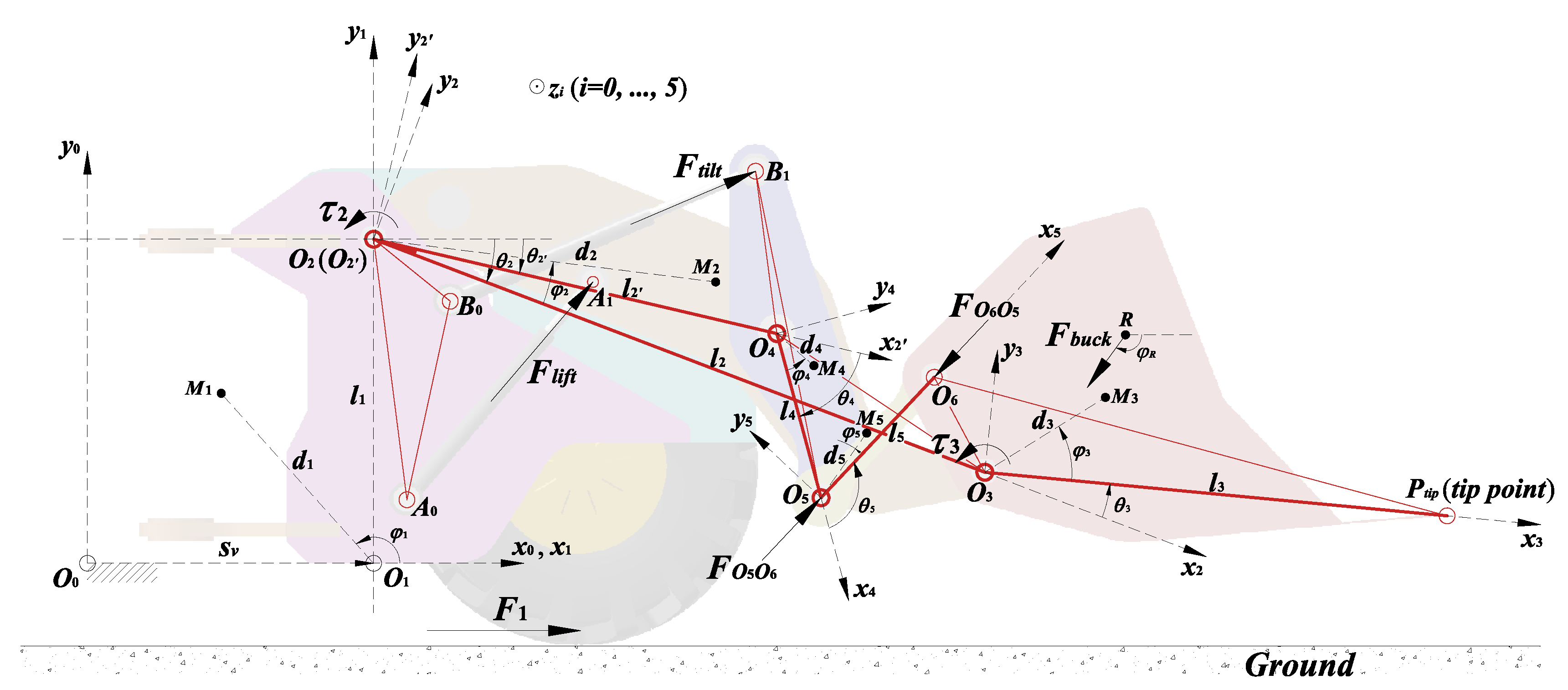
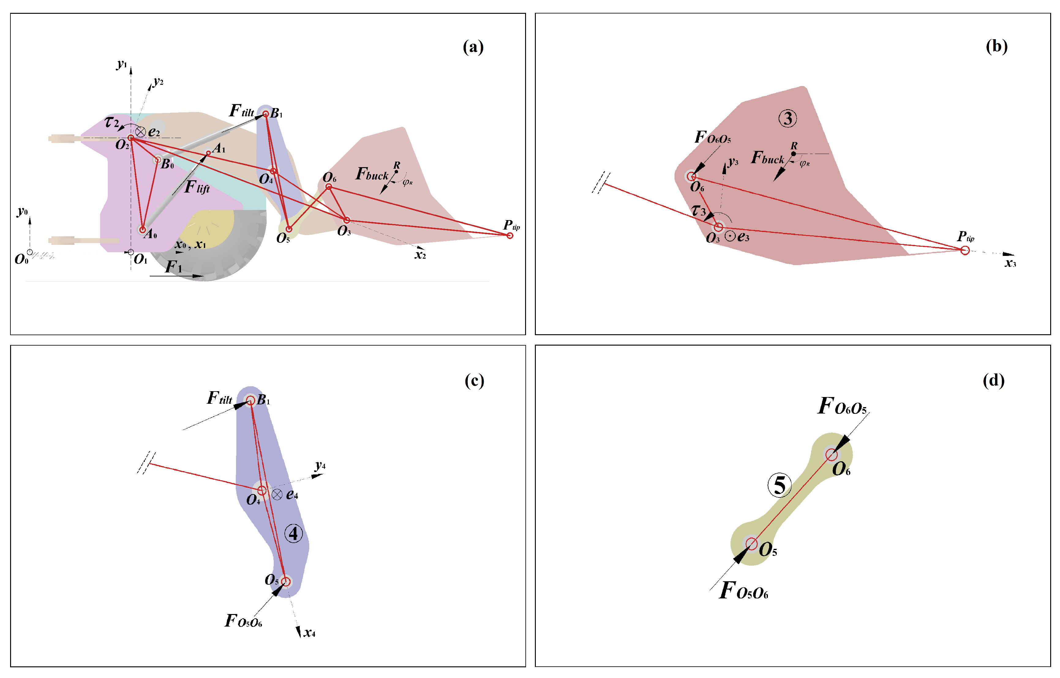
4. Dynamic Modeling of Working Mechanism System

The complex structure of the loader’s working mechanism and the vehicle’s motion lead to strong dynamic coupling. Firstly, the Lagrange method is used in analytical mechanics to fully establish a mechanism dynamic model in joint space considering the vehicle’s motion. Then, the Newton–Euler method is used in vector mechanics to establish the force mapping relations between the joint space and the drive space. Finally, the dynamic model of the mechanism in drive space is obtained.

4.1. Dynamic Model Based on Lagrange Method

The mechanism system is considered as a complete and ideal restraint rigid system with the generalized coordinates s v , θ 2 , θ 3 . As mentioned at the beginning, the working surface (ground) on which the vehicle is traveling is not a level surface, i.e., there may be uphill or downhill roads in practical application. This condition results in the pitch motion of the vehicle, which has a great influence on the effect of the system’s gravity in the dynamic model. Therefore, it is necessary to consider the pitch angle of the vehicle in the Earth’s inertial system. Figure 3 shows the pitch motion of the vehicle relative to the Earth’s inertial system O ˜ x ˜ y ˜ z ˜ . Angle φ 0 is the inclination of the working surface to the level surface and can be regarded as the pitch angle of the vehicle. In practical application, the angle φ 0 can be obtained by an inclination sensor installed on the vehicle.
In Figure 4, in order to make the mathematical symbols neat and uniform, m i represents the mass of the body i i = 1 , , 5 ; M i represents the mass center of the body i; d i represents the vector l O i M i ; and φ i represents the rotation angle of d i relative to x i -axis. The bucket force can be expressed as follows:
F b u c k = F b u c k , x 0 , F b u c k , y 0 T F b u c k , x 0 = F b u c k cos φ R F b u c k , y 0 = F b u c k sin φ R
where F b u c k is considered as the equivalent force exerted by the operating load on the bucket; F b u c k , x 0 and F b u c k , y 0 are the component forces of F b u c k on x 0 -axis and y 0 -axis in the coordinate frame O 0 x 0 y 0 z 0 , respectively; Point R is the equivalent action point of F b u c k on the bucket; and Angle φ R is the direction angle of F b u c k in the coordinate frame O 0 x 0 y 0 z 0 .
For any mechanical systems, the Lagrange function L is defined as follows [31]:
L = E K E P
where E K represents the total kinetic energy of the system and E P represents the total potential energy of the system. Then, the Lagrange dynamic equation of the system’s dynamic state, described by the Lagrange function L, is given by [31]:
Q i = d d t L Θ ˙ i L Θ i i = 1 , , n
where Θ i is the generalized coordinate in the system; Θ ˙ i is the generalized velocity; and Q i is the non-conservative generalized force on the i-th generalized coordinate.
Considering that the Equation (17) does not explicitly contain Θ ˙ i , Equation (17) can be expressed as follows:
Q i = d d t E k Θ ˙ i E k Θ i + E p Θ i
Note that the kinetic energy and the potential energy of each body can be obtained separately. So, Equation (18) can be further expressed as follows:
Q i = j = 1 n d d t E k j Θ ˙ i j = 1 n E k j Θ i + j = 1 n E p j Θ i
The kinetic energy E k j and the potential energy E p j of each body can be given by [27,31]:
E k j = 1 2 j v M j T m j j v M j + 1 2 j ω j T M I j j ω j E p j = m j g ˜ T l ˜ O 0 M j
where j v M j is the velocity of the mass center M j of the body j in the coordinate frame O j x j y j z j ; j ω j is the angular velocity of the body j in the coordinate frame O j x j y j z j ; m j R 3 × 3 is the diagonal matrix associated with the mass m j ; M I j R 3 × 3 is the inertia tensor of the body j in the coordinate frame M O j M x j M y j M z j M x j x j , M y j y j , M y j y j at its mass center M j , which is a symmetric matrix; l ˜ O 0 M j is the vector l O 0 M j in the Earth’s inertial frame O ˜ x ˜ y ˜ z ˜ ; and g ˜ is the acceleration vector of gravity in the Earth’s inertial frame O ˜ x ˜ y ˜ z ˜ . Thus, there are the following expressions:
m j = m j 0 0 0 m j 0 0 0 m j M I j = M I j x M I j x y M I j x z M I j y x M I j y M I j y z M I j z x M I j z y M I j z g ˜ = 0 , g , 0 T l ˜ O 0 M j = R 1 , 0 i = 1 j R 0 , i i 1 l i 1 + R 0 , j j d j
where M I j x , M I j y , and M I j z are the moments of inertia of body j relative to the M x j -axis, M y j -axis, and M z j -axis, respectively, and M I j x y M I j y x , M I j x z M I j z x , and M I j y z M I j z y are the products of inertia; g is the magnitude of the gravity acceleration vector; and R 1 , 0 is the transformation matrix from the ground coordinate frame O 0 x 0 y 0 z 0 to the Earth’s inertial reference frame O ˜ x ˜ y ˜ z ˜ . Combined with Equation (2) and Figure 3, R 1 , 0 can be obtained by the following equation:
R 1 , 0 = I + 1 cos φ 0 0 e ˜ 0 2 + 0 e ˜ 0 sin φ 0
In Equation (22), note that 0 e 0 = 0 , 0 , 1 T and 0 e ˜ 0 R 3 × 3 is the skew-symmetric matrix [27,28] associated with the vector 0 e 0 .
Combined with Equations (4), (6), and (20)–(22), in Figure 4, for the kinematic chains 1 i = 1 , 2 , 3 and 2 i = 1 , 2 , 4 , 5 , the kinetic energy and the potential energy of the mechanism system can be expressed in the following forms:
E k = E k 1 E k 5 = 1 E k D 5 × 5 s ˙ v 2 θ ˙ 2 2 θ ˙ 5 2 + 2 E k D 5 × 10 s ˙ v θ ˙ 2 s ˙ v θ ˙ 3 θ ˙ 4 θ ˙ 5
E p = E p 1 E p 5 = E p D 5 × 5 m 1 g m 5 g
where 1 E k D 5 × 5 and E p D 5 × 5 are the R 5 × 5 matrices, respectively, and 2 E k D 5 × 10 is the R 5 × 10 matrix.
To facilitate the characterization of the dynamic model, in the following equations, s i + j + n and c i + j + n represent sin i + j + n and cos i + j + n , respectively. s i j n and c i j n represent sin ( θ i + θ j + + θ n ) and cos ( θ i + θ j + + θ n ) , respectively. s i j n + i j n and c i j n + i j n represent sin θ i + θ j + + θ n + φ i + φ j + + φ n and cos θ i + θ j + + θ n + φ i + φ j + + φ n , respectively. Note the directions of the vectors and angles. In further considerations, the notations θ i and φ i will be represented as signed angles, that is, it is specified that they are positive in the positive direction of the z i -axis.
Unlike open kinematic chains, the mechanism system in this paper belongs to the category of closed six-link chains. Although it is divided into two kinematic chains to facilitate dynamic modeling and characterization, there are still many couplings, e.g., θ 4 and θ 5 have nonlinear relations with θ 3 . As a result, the analytical equations of Lagrange function L and its partial derivatives are still complicated. In practical application, the overall size and mass of body 5 are relatively tiny, so its inertia force has little effect on the system compared with the driving force, load and other bodies. In addition, the booms rise and the bucket flips inward during the shoveling operation of the mechanism, so the attitude of body 4 changes slightly (tiny swing) with respect to the working surface. Therefore, the motion of body 4 is considered as a plane translation and the kinetic energy of body 5 is neglected to facilitate the solution, which is validated in the final section that the neglected parts have little effect on the whole system. Thus, the non-zero items of the matrices 1 E k D 5 × 5 and 2 E k D 5 × 10 in Equation (23) are, respectively, as follows:
1 E k D i 1 = m i / 2 , i = 1 , , 4 1 E k D i i = m i d i 2 + M I i z / m i / 2 , i = 2 , 3 1 E k D 32 = m 3 l 2 2 + d 3 2 + 2 l 2 d 3 c 3 + 3 + M I 3 z / m 3 / 2 1 E k D 42 = m 4 l 2 2 / 2
2 E k D 21 = m 2 d 2 s 2 + 2 2 E k D 31 = m 3 l 2 s 2 + d 3 s 23 + 3 2 E k D 32 = m 3 d 3 s 23 + 3 2 E k D 35 = m 3 d 3 2 + l 2 d 3 c 3 + 3 + M I 3 z / m 3 2 E k D 41 = m 4 l 2 s 2
The non-zero items of the matrix E p D 5 × 5 in Equation (24) are as follows:
E p D 11 = s v s φ 0 + d 1 s φ 0 + φ 1 E p D 22 = s v s φ 0 + l 1 c φ 0 + d 2 s 2 + 02 E p D 33 = s v s φ 0 + l 1 c φ 0 + l 2 s 2 + 0 + d 3 s 23 + 03 E p D 44 = s v s φ 0 + l 1 c φ 0 + l 2 s 2 + 0 + d 4 s 2 4 + 04 E p D 55 = s v s φ 0 + l 1 c φ 0 + l 2 s 2 + 0 + l 4 s 2 4 + 0 + d 5 s 2 45 + 05
Combined with Equations (19) and (23)–(27), after strict derivation, the dynamic equations of the non-conservative generalized forces Q Q 1 , Q 2 , Q 3 in the generalized coordinates Θ s v , θ 2 , θ 3 are obtained as follows:
Q = Q 1 Q 2 Q 3 = 1 D 3 × 3 s ¨ v θ ¨ 2 θ ¨ 3 + 2 D 3 × 3 s ˙ v 2 θ ˙ 2 2 θ ˙ 3 2 + 3 D 3 × 3 s ˙ v θ ˙ 2 s ˙ v θ ˙ 3 θ ˙ 2 θ ˙ 3 + 4 D 3 × 5 m 1 g m 5 g
where 1 D 3 × 3 , 2 D 3 × 3 and 3 D 3 × 3 are the R 3 × 3 matrices, respectively; 4 D 3 × 5 is the R 3 × 5 matrix.
The items of the matrices 1 D 3 × 3 , 2 D 3 × 3 , and 3 D 3 × 3 are, respectively, as follows:
1 D 11 = m i 1 D 22 = m 2 d 2 2 + M I 2 z / m 2 + m 3 l 2 2 + d 3 2 + 2 l 2 d 3 c 3 + 3 + M I 3 z / m 3 + m 4 l 2 2 1 D 33 = m 3 d 3 2 + M I 3 z / m 3 1 D 12 = 1 D 21 = m 2 d 2 s 2 + 2 m 3 l 2 s 2 + d 3 s 23 + 3 m 4 l 2 s 2 1 D 13 = 1 D 31 = m 3 d 3 s 23 + 3 1 D 23 = 1 D 32 = m 3 d 3 2 + l 2 d 3 c 3 + 3 + M I 3 z / m 3
2 D 12 = m 2 d 2 c 2 + 2 m 3 l 2 c 2 + d 3 c 23 + 3 m 4 l 2 c 2 2 D 13 = m 3 d 3 c 23 + 3 2 D 23 = 2 D 32 = m 3 l 2 d 3 s 3 + 3 2 D i i = 2 D i 1 = 0 , i = 1 , , 3
3 D 13 = 2 m 3 d 3 c 23 + 3 3 D 23 = 2 m 3 l 2 d 3 s 3 + 3 3 D i i = 3 D i 1 = 3 D i 2 = 0 , i = 1 , , 3
The items of the matrix 4 D 3 × 5 are as follows:
4 D 1 i = s φ 0 , i = 1 , , 5 4 D 22 = d 2 c 2 + 02 4 D 23 = l 2 c 2 + 0 + d 3 c 23 + 03 4 D 24 = l 2 c 2 + 0 + d 4 c 2 4 + 04 4 D 25 = l 2 c 2 + 0 + l 4 c 2 4 + 0 + d 5 c 2 45 + 05 4 D 33 = d 3 c 23 + 03 4 D 34 = d 4 c 2 4 + 04 d θ 4 d θ 3 4 D 35 = l 4 c 2 4 + 0 + d 5 c 2 45 + 05 d θ 4 d θ 3 + d 5 c 2 45 + 05 d θ 5 d θ 3 4 D 21 = 4 D 31 = 4 D 32 = 0
Furthermore, combined with Equations (14) and (28), the non-conservative generalized force Q can be expressed as follows:
Q = Q 1 Q 2 Q 3 = Φ d 1 ( s v , s ˙ v , s ¨ v , l l i f t , l ˙ l i f t , l ¨ l i f t , l t i l t , l ˙ t i l t , l ¨ t i l t )
Next, the Newton–Euler method in vector mechanics will be used to derive the model to build the force mapping relations between the joint space and drive space.

4.2. Dynamic Model Derivation Based on Newton–Euler Method

In Figure 4, the generalized force Q in the joint space has the following form:
Q = Q 1 Q 2 Q 3 = F 1 τ 2 τ 3
where F 1 is the total force of all non-conservative forces driving the vehicle’s motions and τ 2 and τ 3 are the total torques of all non-conservative forces driving the rotation of joints O 2 and O 3 , respectively.
Then, the Newton–Euler method in vector mechanics is used to derive the dynamic model. Based on the overall analysis of the mechanism system (see Figure 5a), the following relations can be obtained:
F 1 = F v e h i c l e + F b u c k , x 0 τ 2 = 2 M l i f t + 2 M t i l t + 2 M b u c k
Based on the analysis for the body 3 (see Figure 5b), the following relation can be obtained:
τ 3 = 3 M O 6 O 5 + 3 M b u c k
in which:
2 M l i f t = l O 2 A 0 × F l i f t 2 M t i l t = l O 2 B 0 × F t i l t 2 M b u c k = 3 M b u c k + l O 2 O 3 × F b u c k 3 M O 6 O 5 = l O 3 O 6 × F O 6 O 5
In Equations (35)–(37), F v e h i c l e is the driving force for the vehicle’s motion; F O 6 O 5 is the generalized force exerted by body 5 on body 3; 2 M l i f t , 2 M t i l t , and 2 M b u c k are the torques of the lift cylinder force F l i f t , the tilt cylinder force F t i l t , and the bucket force F b u c k to the z 2 -axis, respectively; and 3 M O 6 O 5 and 3 M b u c k are the torques of the forces F O 6 O 5 and F b u c k to the z 3 -axis, respectively.
Furthermore, based on the analysis of bodies 4 and 5 (see Figure 5c,d), the following relations can be obtained, respectively:
l O 4 B 1 × F t i l t + l O 4 O 5 × F O 5 O 6 = 0 F O 5 O 6 + F O 6 O 5 = 0
where F O 5 O 6 is the generalized force exerted by body 5 on body 4. In addition, in Equations (37) and (38), there are the following expressions:
l O 2 A 0 × F l i f t = F l i f t l O 2 A 0 sin γ O 2 A 0 A 1 2 e 2 l O 2 B 0 × F t i l t = F t i l t l O 2 B 0 sin γ O 2 B 0 B 1 2 e 2 l O 2 O 3 × F b u c k = F b u c k l O 2 O 3 sin φ R θ 2 2 e 2 l O 3 O 6 × F O 6 O 5 = F O 6 O 5 l O 3 O 6 sin γ O 3 O 6 O 5 3 e 3 l O 4 B 1 × F t i l t = F t i l t l O 4 B 1 sin γ O 4 B 1 B 0 4 e 4 l O 4 O 5 × F O 5 O 6 = F O 5 O 6 l O 4 O 5 sin γ O 4 O 5 O 6 4 e 4
where γ O 2 A 0 A 1 , γ O 2 B 0 B 1 , γ O 3 O 6 O 5 , γ O 4 B 1 B 0 , and γ O 4 O 5 O 6 can be expressed by the cylinder lengths l l i f t and l t i l t (refer to the method in Kinematic description Section, for proof see the literature [6]).
In practical application, the direction of the bucket force F b u c k can be evaluated according to the materials in the bucket at different operation stages [22], that is, φ R can be estimated. In addition, as the lifting height of the boom is limited in shovel operation, F b u c k and l O 2 O 3 are not co-linear, that is, sin ( φ R θ 2 ) 0 . Based on this, combined with Equations (33)–(39), F b u c k can be calculated as follows:
F b u c k = 2 M b u c k 3 M b u c k l O 2 O 3 sin φ R θ 2
Then, based on Equations (15), (34), (35), and (40), there are the following expressions:
F v e h i c l e = Q 1 F b u c k , x 0 F b u c k , x 0 = F b u c k cos φ R F b u c k , y 0 = F b u c k sin φ R
Finally, combined with Equations (33) and (41), the following form of dynamics mapping relation can be obtained:
F = F v e h i c l e F b u c k , x 0 F b u c k , y 0 = Φ d 2 ( s v , s ˙ v , s ¨ v , l l i f t , l ˙ l i f t , l ¨ l i f t , l t i l t , l ˙ t i l t , l ¨ t i l t , F l i f t , F t i l t )
In this section, the dynamic model of the working mechanism in drive space is established (Equation (42)). In practical application, when the vehicle displacement, the cylinder lengths and the hydraulic pressures of cylinders are observed, information such as the vehicle’s driving force and the bucket force of the loader can be accurately calculated based on the dynamic model.

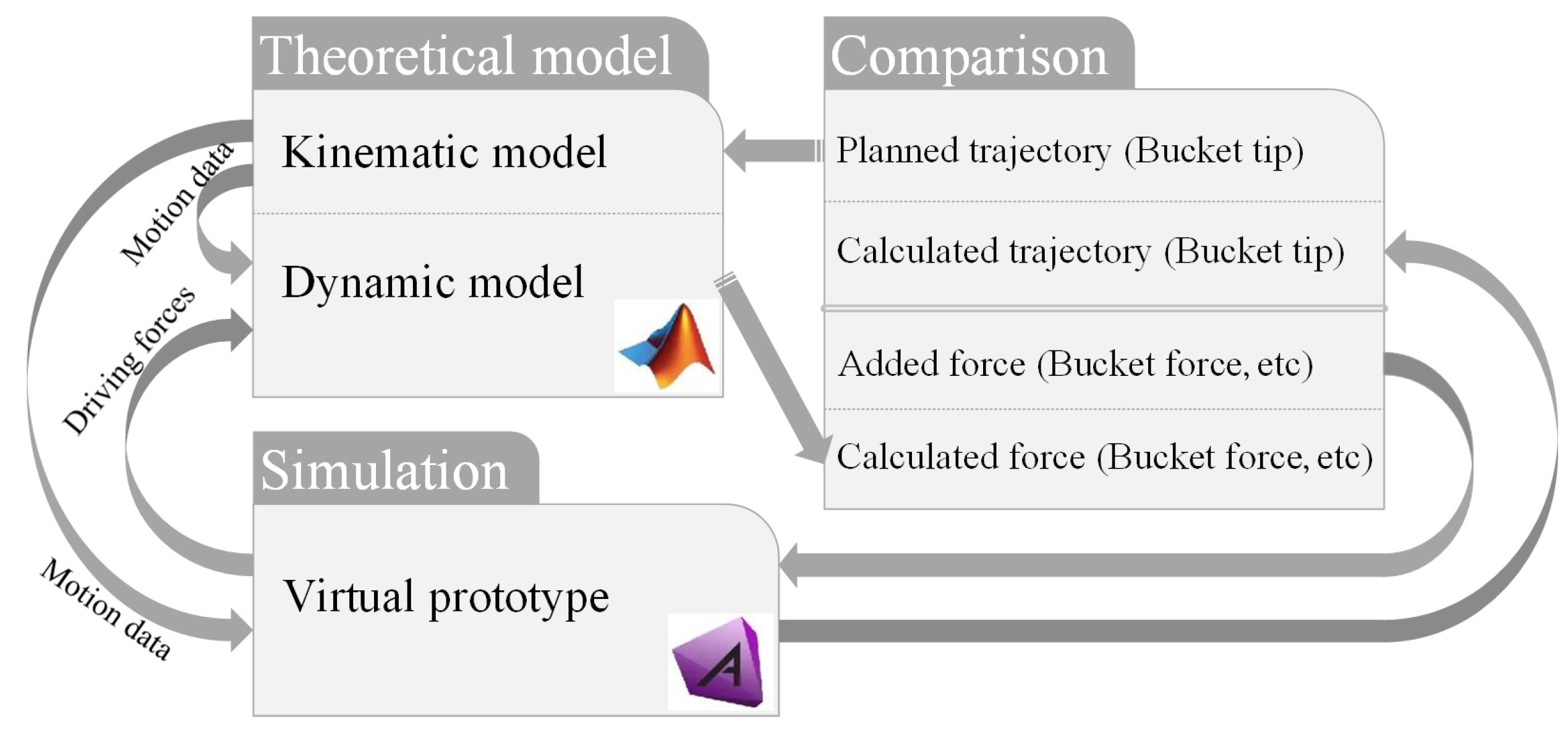
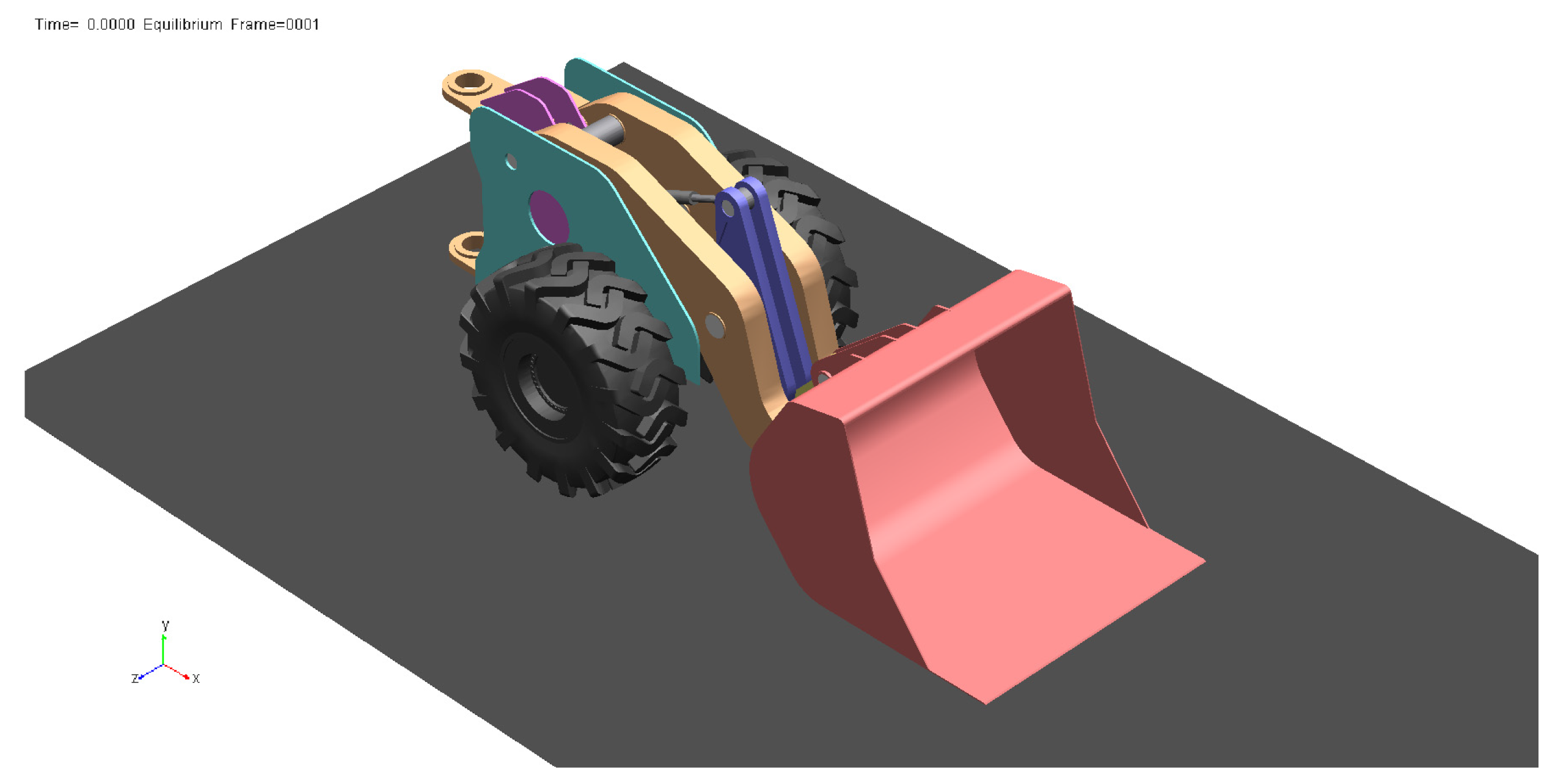
5. Validation and Analysis

In practical application, it is difficult to directly and accurately observe the bucket force. So, the simulation method is adopted to validate and analyze the dynamic model by building a reliable simulation platform (Figure 6).

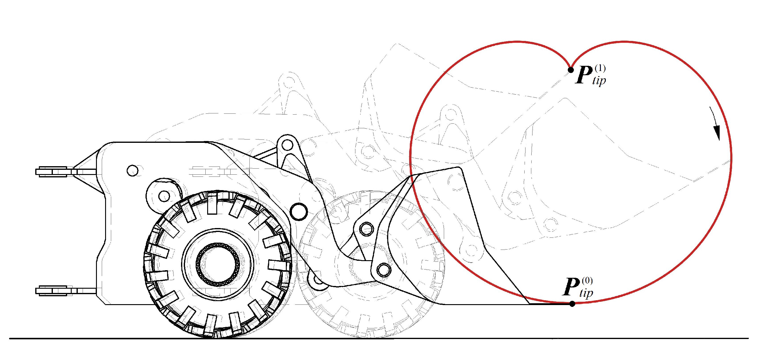
5.1. Validation of the Kinematic Model

Firstly, the kinematic model is validated separately to prove that the kinematic model has no disturbance effect on the dynamic modeling. Following the outline of the counterclockwise outer chain in Figure 6, a virtual prototype based on a 4- m 3 underground loader is created in the dynamic simulation software ADAMS (see Figure 7). The setting parameters, such as the dimensions and constraints of the virtual prototype, can be seen in the literature [6]. Considering the cooperative motion of the vehicle and mechanism, the Cartesian curve is taken as an example of the planned trajectory of the bucket tip P t i p , and the motion data can be calculated by the inverse solution of the kinematic model (Equations (6), (7), and (14)). Then, the motion data are used to move the vehicle body and the cylinder pistons of the virtual prototype to achieve the kinematic simulation. The post-processing module of simulation can directly give the trajectory data (called ’calculated trajectory’) of the bucket tip P t i p . Finally, the calculated trajectory is compared with the planned trajectory to validate the kinematic model. The Cartesian curve function is as follows:
ρ = ζ 1 sin θ
In Figure 8, the bucket tip P t i p is planned to start from the lowest point P t i p 0 (initial position) of the Cartesian curve, move clockwise for one cycle and return to the initial position. At the same time, the attitude angle θ P t i p of the bucket rotates counterclockwise from the initial angle θ P t i p 0 (bucket bottom is flat), reaches the maximum angle θ P t i p 1 at the center point P t i p 1 of the Cartesian curve, and then rotates clockwise to return to the initial angle. For this, the planned trajectory function of the bucket tip P t i p is as follows:
x P t i p = ζ 1 sin θ cos θ + x P t i p 0 y P t i p = ζ 1 sin θ sin θ + 2 ζ + y P t i p 0 θ = 3 π / 2 2 π t / t max θ P t i p = θ P t i p 1 θ P t i p 0 2 t / t max 1 2 + θ P t i p 1
where x P t i p , y P t i p , and θ P t i p are the position and attitude parameters of the bucket tip P t i p at any t time in the coordinate frame O 0 x 0 y 0 z 0 , and x P t i p 0 , y P t i p 0 , and θ P t i p 0 are the initial values. Then, the characteristic coefficient ζ of the Cartesian curve is set to 1, the total time t max is set to 10 s, and the maximum attitude angle θ P t i p 1 of the bucket is set to 0.6 radians.
Based on the kinematic model (Equations (6), (7), and (14)), the motion data (e.g., see the acceleration data in Figure 9) of the vehicle body and the lift and tilt cylinders of the loader are calculated by the inverse solution of the planned trajectory (Equation (44)) of the bucket tip P t i p . Then, the motion data are added to the drivers of the vehicle body and the cylinder pistons of the virtual prototype for kinematic simulation. The post-processing module of simulation directly gives the motion trajectory (calculated trajectory) of the bucket tip P t i p . The calculated trajectory is compared with the planned trajectory (see Figure 10), which shows that the whole process is highly consistent. Figure 11 shows the absolute errors of the x and y coordinates of the calculated trajectory of bucket tip P t i p . It can be seen that the average absolute error of the x coordinate of calculated trajectory is 1.38 × 10 4 m with a maximum absolute error of 2.48 × 10 4 m, not exceeding 0.04‰ of the x coordinate of the planned trajectory. The average absolute error of the y coordinate of the calculated trajectory is 5.22 × 10 5 m with a maximum absolute error of 1.14 × 10 4 m, not exceeding 0.05‰ of the y coordinate of the planned trajectory. These errors can be neglected; thus, the accuracy of the kinematic model is validated.

5.2. Validation and Analysis of the Dynamic Model

Furthermore, the dynamic model is validated and analyzed. Following the outline of the clockwise inner chain in Figure 6, in the motion process of the above virtual prototype, dynamic simulation is carried out by adding a variable force (called ’added force’) on the bucket at any position in the bucket. The post-processing module of simulation can directly obtain the driving force data of the vehicle body and the cylinder pistons. Then, the driving forces data and the motion data of the cylinder pistons are written into the dynamic model (Equation (42)) to calculate the vehicle driving force and the bucket force (called ’calculated force’). Finally, the calculated forces are compared and analyzed with the added force to validate the dynamic model. In addition, the existing dynamic models are also added for comparative analysis to validate the higher accuracy of the dynamic model built in this paper.
Corresponding to the introduction, the existing dynamic models of the loader’s working mechanism can be roughly divided into the following three categories:
(1) Without considering the influence of the vehicle motion, the working mechanism is simplified as the dynamic model of a two-bar mechanism (only the boom and the bucket) [5,7,8,9,10] called ’Model 1’. This model is usually built in the joint space and often neglects the tilt cylinder’s action (affected by the offset load) when switching to the drive space. For this, the Equations (29), (30), (35), and (36) corresponding to such a model can be described as follows:
1 D 12 = m 2 d 2 s 2 + 2 m 3 l 2 s 2 + d 3 s 23 + 3 1 D 13 = m 3 d 3 s 23 + 3 1 D 22 = m 2 d 2 2 + M I 2 z / m 2 + m 3 l 2 2 + d 3 2 + 2 l 2 d 3 c 3 + 3 + M I 3 z / m 3 1 D 33 = m 3 d 3 2 + M I 3 z / m 3 1 D 23 = 1 D 32 = m 3 d 3 2 + l 2 d 3 c 3 + 3 + M I 3 z / m 3 1 D i 1 = 0 , i = 1 , , 3
2 D 12 = m 2 d 2 c 2 + 2 m 3 l 2 c 2 + d 3 c 23 + 3 2 D 13 = m 3 d 3 c 23 + 3 2 D 23 = 2 D 32 = m 3 l 2 d 3 s 3 + 3 2 D i i = 2 D i 1 = 0 , i = 1 , , 3
F 1 = F v e h i c l e + F b u c k , x 0 τ 2 = 2 M l i f t + 2 M b u c k τ 3 = 3 M b u c k
(2) Without considering the influence of the vehicle motion, a simplified dynamic or static model of the working mechanism with some dynamic compensation [6,11,12,13,14,15,16,17,18,19,20,21,22,23] called ’Model 2’ is established. This model is built in the drive space and incorporates the dynamic effects of the boom and the offset load. For this, the Equations (29)–(31) corresponding to such a model can be described as follows:
1 D 12 = m 2 d 2 s 2 + 2 m 3 l 2 s 2 + d 3 s 23 + 3 m 4 l 2 s 2 1 D 22 = m 2 d 2 2 + M I 2 z / m 2 + m 3 l 2 2 + d 3 2 + 2 l 2 d 3 c 3 + 3 + M I 3 z / m 3 + m 4 l 2 2 1 D 32 = m 3 d 3 2 + l 2 d 3 c 3 + 3 + M I 3 z / m 3 1 D i 1 = 1 D i 3 = 0 , i = 1 , , 3
2 D 12 = m 2 d 2 c 2 + 2 m 3 l 2 c 2 + d 3 c 23 + 3 m 4 l 2 c 2 2 D 32 = m 3 l 2 d 3 s 3 + 3 2 D i i = 2 D i 1 = 2 D i 3 = 0 , i = 1 , , 3
3 D i j = 0 , i , j = 1 , , 3
(3) Considering the influence of the vehicle motion, a static model of the working mechanism is established [2,24,25]. The working mechanism of the loader in references [2,24,25] is not exactly the same as that in this study, but their dynamic mechanism models can be classified as a kind of static model that only considers the influence of the vehicle motion but not the dynamic influence of the front-end mechanism. So, a similar model (called ’Model 3’) is built for the reverse six-linkage mechanism in this study drawing on the kind of modeling method in the references [2,24,25] to describe such models. As a comparison group, it is also convenient to analyze the effect caused by various factors more comprehensively and sufficiently in the following text. For this, the Equations (29)–(31) corresponding to such a model can be described as follows:
1 D 11 = m i 1 D 21 = m 2 d 2 s 2 + 2 m 3 l 2 s 2 + d 3 s 23 + 3 m 4 l 2 s 2 1 D 31 = m 3 d 3 s 23 + 3 1 D i 2 = 1 D i 3 = 0 , i = 1 , , 3
2 D i j = 0 , i , j = 1 , , 3
3 D i j = 0 , i , j = 1 , , 3
The dynamic model (Equation (42)) built in this study is called ’Model Novel’ (Model N).
The variable force added on the bucket of the prototype can be expressed as follows:
F b u c k = ξ sin ( π t ) φ R = 3 π / 2
where the characteristic coefficient ξ is set to 50 KN.
The dynamic simulation is carried out (see Figure 12). The driving force data of the vehicle body and the lift/tilt cylinders are obtained directly by the post-processing module (see Figure 13). Then, the driving force data and the motion data of the vehicle body and lift and tilt cylinders are written into Models 1∼3 and Model N, respectively; thus, the vehicle driving force and the bucket force of each model are calculated. Finally, the calculated forces are compared with the added force and the absolute errors are given (see Figure 14, Figure 15 and Figure 16). Table 1 shows the comparison of the average absolute errors ( e r r o r a v g ) and the maximum absolute errors ( e r r o r m a x ) for all models.
In the whole process, the vehicle body and the front-end mechanism move together, and the added force value changes sinusoidally from 0 KN to 50 KN. Combined with Figure 14 and Table 1, in Models 1 and 2, the average absolute errors of the calculated driving force of the vehicle body are 11,018.17 N and 11,314.74 N, respectively, and the maximum absolute errors are 29,347.76 N and 27,032.53 N, respectively. Combined with Figure 9, it can be seen that the excessive errors are sensitive to the acceleration of the vehicle body, which is mainly caused by ignoring the inertia forces generated by the vehicle body motion. In Model 3, the average absolute error of the calculated driving force of the vehicle body is 328.40 N, and the maximum absolute error is 748.03 N. Due to the consideration of the influence of the vehicle motion, the errors perform well, but combined with Figure 9, it can be seen that the errors are sensitive to the acceleration of the front-end mechanism, which is mainly caused by ignoring the inertia forces generated by the front-end mechanism motion. In Model N, the calculated driving force of the vehicle body is highly consistent with the reference driving force in the whole process, with an average absolute error of 55.72 N and a maximum absolute error of 117.95 N. Compared with Models 1∼3, the average and maximum absolute errors of the calculated driving force of the vehicle body of Model N do not exceed 20% of the corresponding errors.
Combined with Figure 15 and Figure 16 and Table 1, in Model 1, the average absolute error of the calculated bucket force in the x direction is 1271.63 N with a maximum absolute error of 4372.93 N, and the average absolute error of the calculated bucket force in the y direction is 2202.52 N with a maximum absolute error of 7574.14 N. The reason for the excessive absolute errors is mainly caused by ignoring the tilt cylinder force (affected by the offset load) and the inertia force generated by the motions of the vehicle body and some components. In Model 2, the average absolute error in the x direction is 322.52 N with a maximum absolute error of 946.42 N, and the average absolute error in the y direction is 558.62 N with a maximum absolute error of 1639.25 N. Due to the dynamic compensation of the front-end mechanism, the errors perform well, but combined with Figure 9, it can be seen that the errors are sensitive to the acceleration of the vehicle body and front-end mechanism, which is mainly caused by ignoring the inertial forces generated by the motions of the vehicle body and some of the components. In Model 3, the average absolute error in the x direction is 467.70 N with a maximum absolute error of 1074.77 N, and the average absolute error in the y direction is 810.08 N with a maximum absolute error of 1861.56 N. Combined with Figure 9, it can be seen that the errors are sensitive to the acceleration of the front-end mechanism, which is mainly caused by ignoring the inertia forces generated by the front-end mechanism motion. In Model N, the calculated bucket force is highly consistent with the added force in the whole process. The average absolute error in the x direction is 23.26 N with a maximum absolute error of only 63.96 N, and the average absolute error in the y direction is 40.30 N with a maximum absolute error of only 110.79 N. Compared with Models 1∼3, the average and maximum absolute errors of the calculated bucket force of Model N do not exceed 10% of the corresponding errors.
In conclusion, the above comparison test fully proves that the dynamics of the vehicle body and front-end mechanism and the force of the tilt cylinder play important roles in improving the model’s accuracy. The dynamic model of the working mechanism system built in this study is superior to the existing dynamic models since it is of higher accuracy and is more suitable for the cooperative motion of the vehicle body and the front-end mechanism.

6. Conclusions

Taking a reverse six-linkage loader as the research object, a kinematic model of the loader’s working mechanism is firstly given. Then, on this basis, an accurate dynamic model of the loader’s working mechanism considering the influence of vehicle motion is established in the 3-DOF motion. Finally, the mapping relations between the vehicle driving force, the bucket force, and the drive space parameters are given.
Since it is difficult to directly and accurately observe the bucket force in practical application, the model in this paper is validated by adding a variable force on the bucket in a simulation platform. In the simulation, the vehicle body and the front-end mechanism move together, and the added force on the bucket changes sinusoidally from 0 KN to 50 KN. The calculated force values based on the established model are highly consistent with the added force values in the whole process. Compared with the existing models, the average and maximum absolute errors of the vehicle driving force calculated by the established model do not exceed 20% of the existing model errors, and the average and maximum absolute errors of the bucket force calculated by the established dynamic model do not exceed 10% of the existing model errors. So, it also proves that the factors, e.g., the dynamics of the vehicle body and front-end mechanism and the force of the tilt cylinder, play important roles in improving the model’s accuracy. The established dynamic model is superior to the existing dynamic models, since it is of higher accuracy and more suitable for the cooperative motion with the vehicle body.
This paper provides important theoretical and practical value for research on the precise online detection of load, the precise identification of mechanical parameters (e.g., system inertia), the optimization of structural design, the identification of vehicle driving force distribution, etc. It provides a reliable basic model for the load detection system of an Intelligent Loader, which can directly and quickly realize the engineering application. The modeling method is also applicable to other mobile multi-bar vehicles. In future work, to better match the conditions of actual loaders, the disturbance effects caused by some non-rigid factors (e.g., the elastic deformation and joint gap of the mechanism, the tire deformation of the vehicle body, changes in the ground, etc.) need to be considered in the model in combination with the mechanism characteristics and operation data of the actual loader, so as to optimize the model to a greater extent. Moreover, in practical application, the model will certainly be applied to the control system of the mechanism for load detection, so the robustness and stability of the model in the control system also need to be further analyzed. The references [32,33] have given good methods and ideas to deal with the above problems.

Author Contributions

Conceptualization, L.L.; methodology, G.L. and G.B.; software, G.L.; validation, G.L. and G.B.; formal analysis, G.L.; investigation, G.B.; resources, L.L.; data curation, H.F.; writing—original draft preparation, G.L.; writing—review and editing, Y.M.; visualization, Y.C.; supervision, L.L.; project administration, Y.M.; funding acquisition, L.L. All authors have read and agreed to the published version of the manuscript.

Funding

This research was funded by the National Key Research and Development Program of China grant numbers 2019YFC0605300 and 2018YFE0192900 and the China Postdoctoral Science Foundation grant number 2022M710354.

Institutional Review Board Statement

Not applicable.

Informed Consent Statement

Not applicable.

Data Availability Statement

Not applicable.

Acknowledgments

The authors wish to acknowledge the support received from the National Key Research and Development Program of China (2019YFC0605300 and 2018YFE0192900) and the China Postdoctoral Science Foundation (2022M710354).

Conflicts of Interest

The authors declare no conflict of interest.

Abbreviations

a P i acceleration vector of any point P i of body i ;
j a P i components of acceleration vector a P i given in coordinate frame O j x j y j z j ;
d i , d i length vector from point O i to point M i ( l O i M i ) and its magnitude ( l O i M i ), respectively;
1 D 3 × 3 , 2 D 3 × 3 , 3 D 3 × 3 , 4 D 3 × 5 matrices of 3 × 3 , 3 × 3 , 3 × 3 and 3 × 5 dimensions for generalized force Q i , respectively;
1 D i j , 2 D i j , 3 D i j , 4 D i j items of matrices 1 D 3 × 3 , 2 D 3 × 3 , 3 D 3 × 3 and 4 D 3 × 5 , respectively;
1 E k D 5 × 5 , 2 E k D 5 × 10 matrices of 5 × 5 and 5 × 5 dimensions for kinetic energy E k i , respectively;
1 E k D i j , 2 E k D i j items of matrices 1 E k D 5 × 5 and 2 E k D 5 × 10 , respectively;
E p D 5 × 5 matrix of 5 × 5 dimensions for potential energy E p i ;
E p D i j items of matrix E p D 5 × 5 ;
e i unit vector of 3 × 3 dimensions on i-th joint axis;
j e i components of unit vector e i given in coordinate frame O j x j y j z j ;
j e ˜ i skew-symmetric matrix associated with vector j e i ;
E K , E P total kinetic energy and total potential energy of system, respectively;
E k i , E p i kinetic energy and potential energy of body i, respectively;
E k , E p matrices of kinetic energy E k i and potential energy E p i , respectively;
F force matrix of F v e h i c l e , F l o a d , x 0 , F l o a d , y 0 ;
F 1 , F 1 total force vector of all non-conservative forces driving the vehicle’s motion and its magnitude, respectively;
F l i f t / F l i f t ( t ) piston force of lift hydraulic cylinder;
F t i l t / F t i l t ( t ) piston force of tilt hydraulic cylinder;
F l o a d , F l o a d equivalent force vector exerted by the working load on the bucket and its magnitude, respectively;
F l o a d , x 0 , F l o a d , y 0 component forces of F l o a d on x 0 -axis and y 0 -axis in coordinate frame O 0 x 0 y 0 z 0 , respectively;
F v e h i c l e , F v e h i c l e driving force vector for vehicle’s motion and its magnitude, respectively;
F O 5 O 6 , F O 5 O 6 generalized force vector exerted by body 5 on body 4 and its magnitude, respectively;
F O 6 O 5 , F O 6 O 5 generalized force vector exerted by body 5 on body 3 and its magnitude, respectively;
gmagnitude of gravity acceleration vector;
g ˜ acceleration vector of gravity given in Earth’s inertial frame O ˜ x ˜ y ˜ z ˜ ;
I identity matrix of 3 × 3 dimensions;
M I j inertia tensor of body j in local coordinate frame M O j M x j M y j M z j ;
M I j x , M I j y , M I j z moments of inertia of body j relative to M x j -axis, M y j -axis and M z j -axis, respectively;
M I j x y / M I j y x , M I j x z / M I j z x , M I j y z / M I j z y products of inertia of body j relative to M x j -axis, M y j -axis and M z j -axis, respectively;
l l i f t / l l i f t ( t ) total length of lift hydraulic cylinder;
l ˙ l i f t , l ¨ l i f t First and second derivatives of l l i f t ( t ) , respectively;
l t i l t / l t i l t ( t ) total length of tilt hydraulic cylinder;
l ˙ t i l t , l ¨ t i l t First and second derivatives of l t i l t ( t ) , respectively;
l i j , l i j length vector from point i to point j and its magnitude, respectively;
l ˙ i j , l ¨ i j First and second derivatives of l i j , respectively;
l i , l i length vector from point O i to point O i + 1 ( l O i O i + 1 ) and its magnitude ( l O i O i + 1 ), respectively;
j l i components of length vector l i given in coordinate frame O j x j y j z j ;
l P i length vector from point O i to point P i ( l O i P i );
j l P i components of length vector l P i given in coordinate frame O j x j y j z j ;
l ˜ O 0 M i components of length vector from point O 0 to point M i ( l O 0 M i ) given in Earth’s inertial frame O ˜ x ˜ y ˜ z ˜ ;
LLagrange function;
m i mass of body i;
m i diagonal matrix of 3 × 3 dimensions associated with mass m i ;
M i mass center point of body i;
i M l i f t , i M t i l t , i M l o a d , i M O 6 O 5 torques of forces F l i f t , F t i l t , F l o a d , and F O 6 O 5 to z i -axis in coordinate frame O i x i y i z i , respectively;
O i x i y i z i coordinate frame on i-th joint fixed to body i;
O ˜ x ˜ y ˜ z ˜ coordinate frame fixed to Earth’s inertial system;
M O j M x j M y j M z j coordinate frame on mass center M j fixed to body j;
P i any point of body i;
P t i p point of bucket tip;
Q i non-conservative generalized force on i-th generalized coordinate;
Q force matrix of Q i ;
Requivalent action point of F l o a d on bucket;
R 1 , 0 transformation matrix from ground coordinate frame O 0 x 0 y 0 z 0 to Earth’s inertial reference frame O ˜ x ˜ y ˜ z ˜ ;
R i , j , R i , j 1 , R i , j T transformation matrix from O j x j y j z j to O i x i y i z i reference frame and its inverse matrix and transposition matrix, respectively;
R k r Rodriguez matrix of 3 × 3 dimensions;
s i + j + n sin i + j + n ;
c i + j + n cos i + j + n ;
s i j n sin ( θ i + θ j + + θ n ) ;
c i j n cos ( θ i + θ j + + θ n ) ;
s i j n + i j n sin θ i + θ j + + θ n + φ i + φ j + + φ n ;
c i j n + i j n cos θ i + θ j + + θ n + φ i + φ j + + φ n ;
s v / s v ( t ) driving displacement of vehicle body;
s ˙ v , s ¨ v First and second derivatives of s v ( t ) respectively;
i s v components of driving displacement vector s v of vehicle body given in coordinate frame O i x i y i z i ;
i s ˙ v , i s ¨ v First and second derivatives of i s v respectively;
ttime variable;
t max total time of a cycle for prototype simulation;
v P i velocity vector of any point P i of body i ;
j v P i components of velocity vector v P i given in coordinate frame O j x j y j z j ;
j v M i velocity vector of mass center M i of body i given in coordinate frame O j x j y j z j ;
x i , y i , z i x i -axis, y i -axis, z i -axis of coordinate frame O i x i y i z i , respectively;
M x j , M y j , M z j x j -axis, y j -axis, z j -axis of coordinate frame M O j M x j M y j M z j , respectively;
x P t i p , y P t i p position coordinates of bucket tip P t i p in coordinate frame O 0 x 0 y 0 z 0 ;
α i angular acceleration of body i ;
j α i components of angular acceleration α i given in coordinate frame O j x j y j z j ;
j α ˜ i skew-symmetric matrix associated with vector j α i ;
γ i j k angle i j k ;
γ ˙ i j k , γ ¨ i j k First and second derivatives of γ i j k respectively;
ζ characteristic coefficient of Cartesian curve function;
θ polar angle of Cartesian curve in polar coordinate frame;
θ i relative rotation angle of body i with respect to body i-1 carried out about the joint axis;
θ ˙ i , θ ¨ i First and second derivatives of θ i , respectively;
θ P t i p attitude angle of bucket tip P t i p in coordinate frame O 0 x 0 y 0 z 0 ;
Θ generalized coordinate matrix of Θ i ;
Θ i , Θ ˙ i generalized coordinate and generalized velocity in system, respectively;
ξ characteristic coefficient of expression about F l o a d ;
ρ polar radius of Cartesian curve in polar coordinate frame;
τ i total torque of all non-conservative forces driving i-th joint rotating;
φ 0 inclination angle of working surface to level surface (regarded as pitch angle of vehicle body);
φ i rotation angle of d i relative to x i -axis;
φ R direction angle of F l o a d in coordinate frame O 0 x 0 y 0 z 0 ;
Φ k 1 , Φ k 2 kinematic mapping functions;
Φ d 1 , Φ d 2 dynamic mapping functions;
ω i angular velocity of body i ;
j ω i components of angular velocity ω i given in coordinate frame O j x j y j z j ;
j ω ˜ i skew-symmetric matrix associated with vector j ω i .

References

  1. Dadhich, S.; Bodin, U.; Andersson, U. Key challenges in automation of earth-moving machines. Autom. Constr. 2016, 68, 212–222. [Google Scholar] [CrossRef] [Green Version]
  2. Gao, G.; Wang, J.; Ma, T.; Han, Y.; Yang, X.; Li, X. Optimisation strategy of torque distribution for the distributed drive electric wheel loader based on the estimated shovelling load. Veh. Syst. Dyn. 2022, 60, 2036–2054. [Google Scholar] [CrossRef]
  3. Backman, S.; Lindmark, D.; Bodin, K.; Servin, M.; Mörk, J.; Löfgren, H. Continuous Control of an Underground Loader Using Deep Reinforcement Learning. Machines 2021, 9, 216. [Google Scholar] [CrossRef]
  4. Dadhich, S. Automation of Wheel-Loaders. Ph.D. Thesis, Luleå University of Technology, Luleå, Sweden, 2018. [Google Scholar]
  5. Gong, J.; Cui, Y. Track planning for a wheel loader in a digging. J. Mech. Eng. 2009, 45, 29–34. [Google Scholar] [CrossRef]
  6. Liang, G.; Liu, L.; Meng, Y.; Gu, Q.; Fang, H. Dynamic modelling and accuracy analysis for front-end weighing system of LHD vehicles. Proc. Inst. Mech. Eng. Part K J. -Multi-Body Dyn. 2021, 235, 514–535. [Google Scholar] [CrossRef]
  7. Gong, J.; Bao, J.; Yi, G.; Cui, Y. Trajectory-following control for manipulator of wheel loaders based on computed torque. J. Mech. Eng. 2010, 46, 141–146. [Google Scholar] [CrossRef]
  8. Kang, H.; Jung, W.; Lee, C. Modeling and Measurement of Payload Mass of the Wheel Loader in the Dynamic State Based on Experimental Parameter Identification; Technical Report, SAE Technical Paper: Warrendale, PA, USA, 2016. [Google Scholar] [CrossRef]
  9. Kudryavcev, E. Modeling of Efforts on Cylinder of Boom Lift of Small Loader. In Proceedings of the IOP Conference Series: Materials Science and Engineering; IOP Publishing: Bristol, UK, 2021; Volume 1079, p. 052045. [Google Scholar] [CrossRef]
  10. Wang, X.; Zhang, H.; Yang, J.; Ge, L.; Hao, Y.; Quan, L. Research on the Characteristics of Wheel Loader Boom Driven by the Asymmetric Pump Controlled System. J. Mech. Eng. 2021, 57, 258–266, 284. [Google Scholar] [CrossRef]
  11. Fales, R.; Spencer, E.; Chipperfield, K.; Wagner, F.; Kelkar, A. Modeling and Control of a Wheel Loader With a Human-in-the-Loop Assessment Using Virtual Reality. J. Dyn. Syst. Meas. Control 2005, 127, 415–423. [Google Scholar] [CrossRef]
  12. Sarata, S.; Osumi, H.; Kawai, Y.; Tomita, F. Trajectory arrangement based on resistance force and shape of pile at scooping motion. In Proceedings of the IEEE International Conference on Robotics and Automation, ICRA’04, New Orleans, LA, USA, 26 April–1 May 2004; Volume 4, pp. 3488–3493. [Google Scholar] [CrossRef]
  13. Takahashi, Y.; Yasuhara, R.; Kanai, O.; Osumi, H.; Sarata, S. Development of bucket scooping mechanism for analysis of reaction force against rock piles. In Proceedings of the 23rd International Symposium on Automation and Robotics in Construction, Zadar, Croatia, 24–27 October 2006; pp. 476–481. [Google Scholar]
  14. Wang, W.; Wang, T.; Zhao, H.; Wei, H. Lean weight about dynamic weighing of loaders. J. Mech. Eng. 2007, 43, 106–110. [Google Scholar] [CrossRef]
  15. Worley, M.; La Saponara, V. A simplified dynamic model for front-end loader design. Proc. Inst. Mech. Eng. Part C Journal Mech. Eng. Sci. 2008, 222, 2231–2249. [Google Scholar] [CrossRef]
  16. Roskam, R.; Dobkowitz, D. Modeling of a front end loader for control design. In Proceedings of the 2015 23rd Mediterranean Conference on Control and Automation (MED), Torremolinos, Spain, 16–19 June 2015; pp. 442–447. [Google Scholar] [CrossRef]
  17. Yung, I.; Freidovich, L.; Vázquez, C. Payload estimation in front-end loaders. In Proceedings of the MCG 2016—5th International Conference on Machine Control & Guidance, Vichy, France, 5–6 October 2016. [Google Scholar]
  18. Lindmark, D.M.; Servin, M. Computational exploration of robotic rock loading. Robot. Auton. Syst. 2018, 106, 117–129. [Google Scholar] [CrossRef] [Green Version]
  19. Wan, Y.; Song, X.; Yu, L.; Yuan, Z. Load Identification Model and Measurement Method of Loader Working Device. J. Vib. Meas. Diagn. 2019, 39, 582–589. [Google Scholar] [CrossRef]
  20. Brinkschulte, L.; Hafner, J.; Geimer, M. Real-time load determination of wheel loader components. Atzheavy Duty Worldw. 2019, 12, 62–68. [Google Scholar] [CrossRef]
  21. Fernando, H.; Marshall, J.A.; Larsson, J. Iterative learning-based admittance control for autonomous excavation. J. Intell. Robot. Syst. 2019, 96, 493–500. [Google Scholar] [CrossRef] [Green Version]
  22. Madau, R.; Colombara, D.; Alexander, A.; Vacca, A.; Mazza, L. An online estimation algorithm to predict external forces acting on a front-end loader. Proc. Inst. Mech. Eng. Part I J. Syst. Control. Eng. 2021, 235, 1678–1697. [Google Scholar] [CrossRef]
  23. Yuan, Z.; Lu, Y.; Hong, T.; Ma, H. Research on the load equivalent model of wheel loader based on pseudo-damage theory. Proc. Inst. Mech. Eng. Part C J. Mech. Eng. Sci. 2022, 236, 1036–1048. [Google Scholar] [CrossRef]
  24. Frank, B.; Kleinert, J.; Filla, R. Optimal control of wheel loader actuators in gravel applications. Autom. Constr. 2018, 91, 1–14. [Google Scholar] [CrossRef]
  25. Sánchez, M.C.; Torres-Torriti, M.; Cheein, F.A. Online Inertial Parameter Estimation for Robotic Loaders. IFAC-PapersOnLine 2020, 53, 8763–8770. [Google Scholar] [CrossRef]
  26. Yuan, Z.; Ma, H.; Lu, Y.; Zhu, S.; Hong, T. The application of load identification model on the weld line fatigue life assessment for a wheel loader boom. Eng. Fail. Anal. 2019, 104, 898–910. [Google Scholar] [CrossRef]
  27. Shabana, A.A. Dynamics of Multibody Systems; Cambridge University Press: Cambridge, UK, 2020. [Google Scholar]
  28. Šalinić, S.; Bošković, G.; Nikolić, M. Dynamic modelling of hydraulic excavator motion using Kane’s equations. Autom. Constr. 2014, 44, 56–62. [Google Scholar] [CrossRef]
  29. Angeles, J.; Ma, O.; Rojas, A. An algorithm for the inverse dynamics of n-axis general manipulators using Kane’s equations. Comput. Math. Appl. 1989, 17, 1545–1561. [Google Scholar] [CrossRef] [Green Version]
  30. Li, Y.; Liu, W.; Frimpong, S. Compound mechanism modeling of wheel loader front-end kinematics for advance engineering simulation. Int. J. Adv. Manuf. Technol. 2015, 78, 341–349. [Google Scholar] [CrossRef]
  31. Lurie, A.I. Analytical Mechanics; Springer Science & Business Media: Berlin, Germany, 2002. [Google Scholar]
  32. Yin, J.; Shen, D.; Du, X.; Li, L. Distributed Stochastic Model Predictive Control With Taguchi’s Robustness for Vehicle Platooning. IEEE Trans. Intell. Transp. Syst. 2022, 23, 15967–15979. [Google Scholar] [CrossRef]
  33. Shen, D.; Chen, Y.; Li, L. State-feedback Switching Linear Parameter Varying Control for Vehicle Path Following Under Uncertainty and External Disturbances. In Proceedings of the 2022 IEEE 25th International Conference on Intelligent Transportation Systems (ITSC), Macau, China, 8–12 October 2022; pp. 3125–3132. [Google Scholar] [CrossRef]
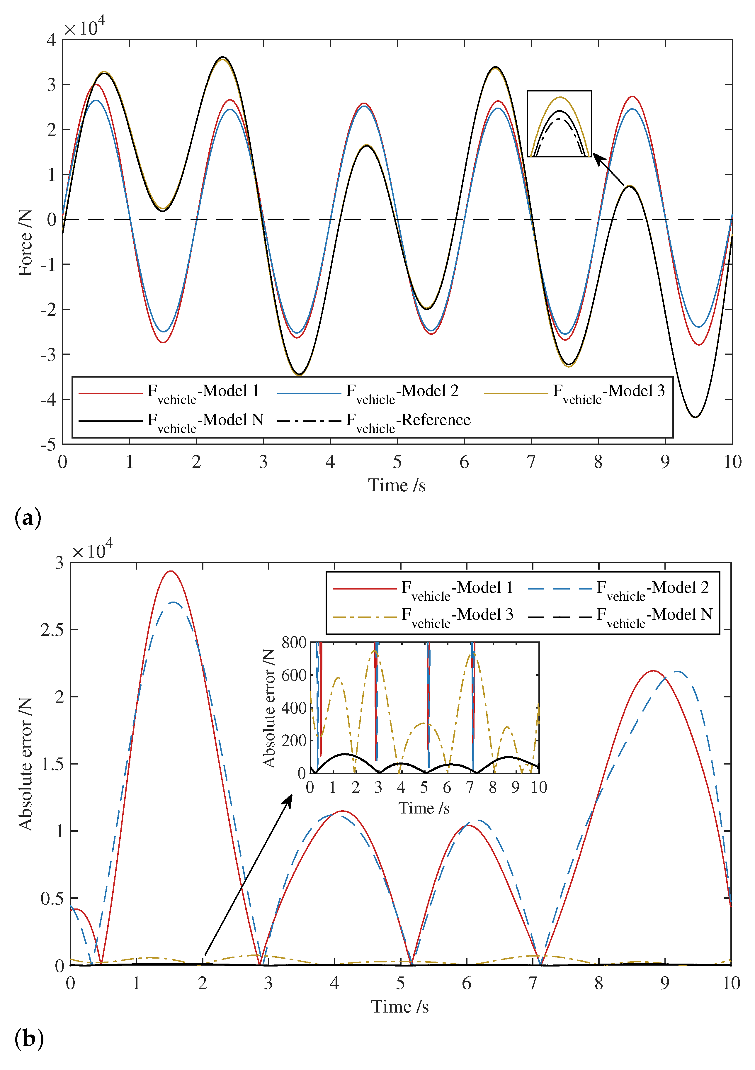
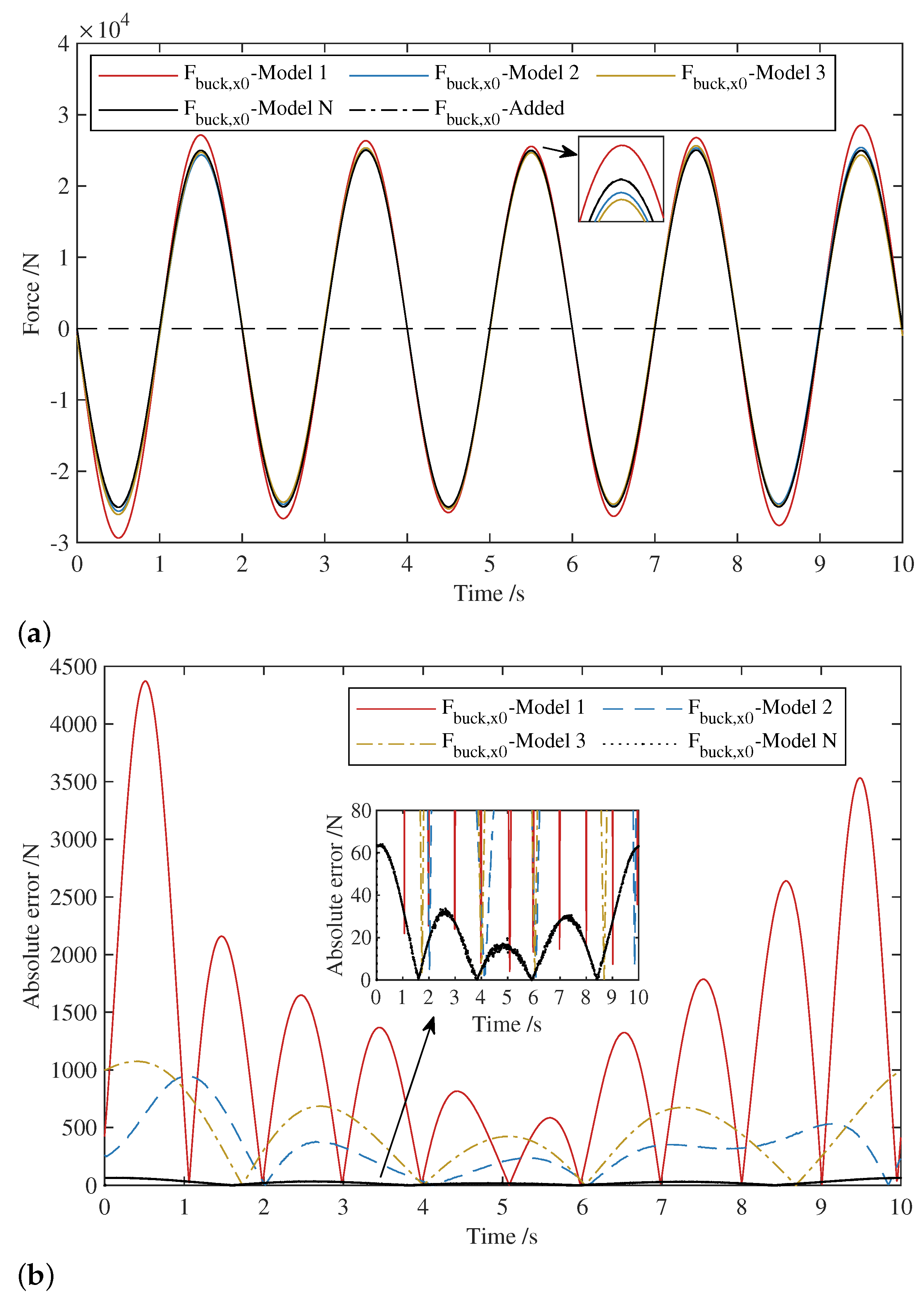
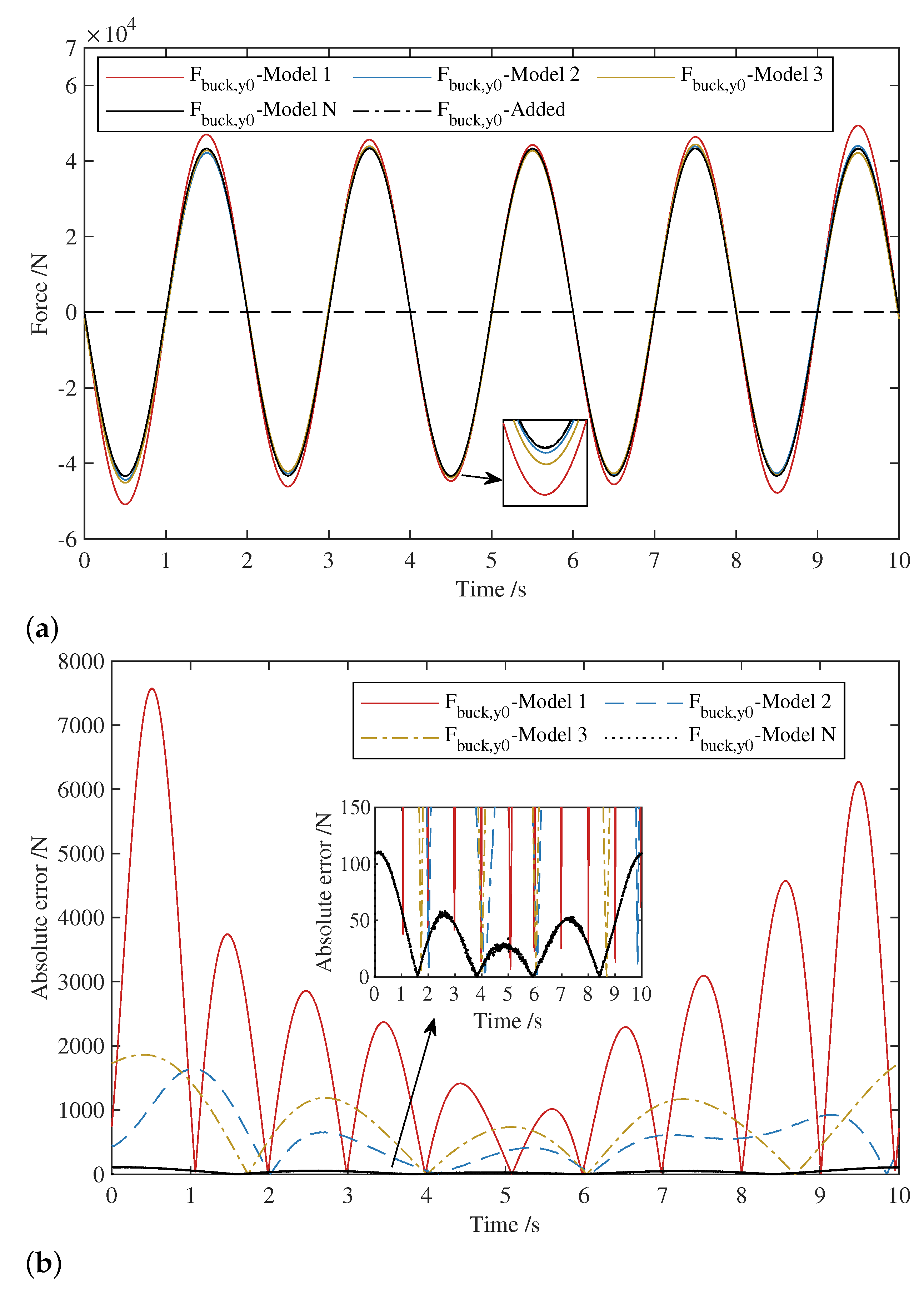
Figure 1. Loader working mechanism system diagram.
Machines 11 00009 g001
Figure 2. Kinematic model of the working mechanism system.
Machines 11 00009 g002
Figure 3. Pitch motion of reference vehicle.
Machines 11 00009 g003
Figure 4. Dynamic model of the working mechanism system.
Machines 11 00009 g004
Figure 5. Multibody model of the working mechanism system. (a) The overall model of the mechanism system; (b) The single model of the body 3; (c) The single model of the body 4; (d) The single model of the body 5.
Machines 11 00009 g005
Figure 6. Simulation platform outline.
Machines 11 00009 g006
Figure 7. Virtual prototype in ADAMS.
Machines 11 00009 g007
Figure 8. Motion process of working mechanism.
Machines 11 00009 g008
Figure 9. Acceleration curves of the vehicle body, lift cylinder, and tilt cylinder.
Machines 11 00009 g009
Figure 10. Comparison between calculated trajectory and planned trajectory of bucket tip P t i p .
Machines 11 00009 g010
Figure 11. Error analysis of calculated trajectory of bucket tip P t i p .
Machines 11 00009 g011
Figure 12. Dynamic simulation process.
Machines 11 00009 g012
Figure 13. Driving forces of vehicle body, lift cylinder, and tilt cylinder.
Machines 11 00009 g013
Figure 14. Comparison and error of vehicle driving force for each model. (a) Comparisons between calculated driving force and reference driving force of the vehicle body; (b) Absolute errors of calculated driving force of the vehicle body.
Machines 11 00009 g014
Figure 15. Comparison and error of bucket force in the x direction for each model. (a) Comparisons in the x direction between calculated bucket force and added force; (b) Absolute errors of calculated bucket force in the x direction.
Machines 11 00009 g015
Figure 16. Comparison and error of bucket force in y direction for each model. (a) Comparisons in y direction between calculated bucket force and added force; (b) Absolute errors of calculated bucket force in the y direction.
Machines 11 00009 g016
Table 1. Absolute error comparison for each model.
Model 1Model 2Model 3Model N
F v e h i c l e 11,018.1711,314.74328.4055.72
E r r o r a v g /N F b u c k , x 0 1271.63322.52467.7023.26
F b u c k , y 0 2202.52558.62810.0840.30
F v e h i c l e 29,347.7627,032.53748.03117.95
E r r o r m a x /N F b u c k , x 0 4372.93946.421074.7763.96
F b u c k , y 0 7574.141639.251861.56110.79
Disclaimer/Publisher’s Note: The statements, opinions and data contained in all publications are solely those of the individual author(s) and contributor(s) and not of MDPI and/or the editor(s). MDPI and/or the editor(s) disclaim responsibility for any injury to people or property resulting from any ideas, methods, instructions or products referred to in the content.

