Research on Fault Diagnosis of Six-Phase Propulsion Motor Drive Inverter for Marine Electric Propulsion System Based on Res-BiLSTM

Abstract

To ensure the implementation of the marine electric propulsion self-healing strategy after faults, it is necessary to diagnose and accurately classify the faults. Considering the characteristics of the residual network (ResNet) and bidirectional long short-term memory (BiLSTM), the Res-BiLSTM deep learning algorithm is used to establish a fault diagnosis model to distinguish the types of electric drive faults. First, the powerful fault feature extraction ability of the residual network is used to deeply mine the fault features in the signals. Then, perform time-series learning through a bidirectional long short-term memory network, and further excavate the transient time-series features in the fault features so as to achieve the accurate classification of drive inverter faults. The effectiveness of the method is verified using noise-free fault data, and the robustness of the method is verified using data with varying degrees of noise. The results show that compared with conventional deep learning algorithms, Res-BiLSTM has the fastest and most stable training process, the diagnostic performance is improved, and the accuracy can be maintained over 95% under 25–19 dB. It has certain robustness and can be applied to marine electric propulsion systems drive inverter fault diagnosis, and its results can provide data support for the implementation of self-healing control strategies.

1. Introduction

With the in-depth research of all-electric ship technology, the research on the safety and reliability of its main power unit, the electric propulsion system, has become a hot spot nowadays. The propulsion motor drive inverter has a much higher failure rate in the electric propulsion system than the motor itself due to its large number of power electronic devices, complex electronic control, and harsh offshore working environment [1]. Once the frequency converter fails, the entire propulsion system will lose its working ability, bringing catastrophic accidents to the ship and endangering the safety of life and property [2]. Therefore, it is of great practical significance to improve the reliability of the propulsion system to study how to quickly find the fault of the drive unit and restrict it in time to reduce the impact of the fault and realize the self-healing of the fault.

The propulsion motor drive, especially the inverter circuit part that realizes the PWM control strategy, is a weak link in the marine electric propulsion system that is prone to faults. In this regard, about 38% of the faults in power conversion circuits occur in semiconductor devices, and IGBTs are the most widely used semiconductor switching devices, and the IGBT’s faults of inverters mainly include open circuit faults and short circuit faults [3]. For the fault diagnosis of the switching devices in the inverter circuits, there are mainly methods based on signal analysis, model reference, and machine learning.

The signal analysis method directly analyzes the electrical signal of the system and is the most widely used fault diagnosis method at present. H Yin et al. [4] design an adaptive real-time fast voltage fault location method based on the voltage signal. The fault location is performed by the average phase voltage deviation of each switching cycle. The fault can be detected and located within one switching cycle, but additional voltage acquisition is required. Considering that the current signal has been collected in the control system, based on the current signal, M. Trabelsi and E. Semail [5] use the current data in the $\mathsf{\alpha }\text{-}\mathsf{\beta }$ reference frame to define the virtual current vector (VCVn) and use the projection of the zero-sequence current on the vector as the fault feature, calculate the fault index, and diagnose the open-circuit fault of the multi-phase PMSM inverter. By introducing VCVn, misdiagnosis caused by changes in system operating conditions can be avoided, and it has high sensitivity and robustness to faults. F Wu et al. [6] simplified the Fourier series of each sampling instant by reconstructing the zero-crossing position data and multiplying them with the reference signal based on the current signal spectrum and use it as a feature for fault diagnosis to improve the diagnosis effect. B. Gmati et al. consider the PMSM drive system under the model predictive control strategy, use the error between the model predicted current and the actual current in the dq reference frame to calculate the diagnostic variables, establish a fuzzy rule, and obtain device fault information through fuzzy logic for fault diagnosis. Compared with the traditional current error diagnosis algorithm, the fuzzy logic algorithm has a short calculation time and robustness against parameters and operating point variation of the system in the literature [7]. However, this type of fault diagnosis method based on electrical signals uses artificially set fault thresholds for alarm and fault tolerance, which is easy to cause false alarms and delays.

The model reference method has the characteristics of fast running speed, good real-time performance, and easy implementation in the control system and has been widely studied. H. Yin et al. [8] designed a current observer to calculate the fault residual, designed an adaptive threshold based on the current dynamic characteristics and the system operating state, and used the current system residual and the average value of the basic period as diagnostic variables for fault diagnosis. C. Chen et al. [9] analyzed the voltage waveform under normal operating conditions, established a hybrid logic dynamic model of the inverter, designed a voltage expansion observer, and determined the faulty device according to the residual error between the observed voltage and the actual voltage. Y. Cheng et al. [10] obtained the expected voltage through a mixed logic dynamic model, estimated the voltage through the measured current, and used the average voltage deviation of each switching cycle as a fault location variable for fault diagnosis. However, such methods require system control signals as model input, and the diagnostic effect is related to the accuracy of the model built. The difficulty in obtaining control signals and the complexity of computation lead to limited practicability.

In recent years, with the rise of artificial intelligence research, knowledge- and data-driven machine learning fault diagnosis methods have become a current research hotspot. H. Sumin et al. [11] used genetic algorithm-rough set reduction (GR) to reduce the dimension of fault features; built a time performance evaluation algorithm (PTA) algorithm to calculate the optimal model and optimized the Bayesian network (BN) diagnostic model. GR-PTA-BN has higher diagnostic accuracy than traditional BP networks, but there are disadvantages such as the long network training time. M. Ali et al. [12] used the probabilistic principal component analysis method to process the output voltage of the inverter and used SVM for fault classification, and the detection accuracy and time were improved. The current spectrum generated by the three-phase current signal preprocessed by PCA is input to the pooling layer of the hybrid convolutional neural network for feature extraction, and the features are combined in the fully connected layer to identify faults, which has high accuracy and strong generalization. However, there are still problems, such as insufficient feature extraction and too high of a dimension, which affect the diagnosis speed [13]. K. Sarita et al. adopted the two-samples technique, used the load impedance and voltage to estimate the current, and realized the fault alarm by the difference between the estimated current and the actual current; used the EWP to extract the features of the inverter output current, and used the SVM to classify the fault. Compared with traditional PCA and WT algorithms, EPW-SVM has a faster diagnosis and more reliable results in the literature [14]. In addition, to solve the problem of data dependence, L. Kou et al. [15] adopted the knowledge-driven method to extract the features of the inverter output current to form a slope data set and then trained the classifier through the random forest algorithm. Y. Xia and Y. Xu [16] used the current signal as the original input and generated the feature set through manifold feature learning. After training the extreme learning machine to form the initial diagnosis model, the model parameters were adjusted to minimize the difference between the source system and the target data distribution to realize the diagnosis model.

In this paper, combining the characteristics of the deep network and recurrent network, a Res-BiLSTM deep learning method was designed to diagnose the fault of the frequency conversion unit driven by the six-phase propulsion system of the ship. According to the current data of the output terminal of the six-phase inverter under different fault conditions, the feature information in the fault data is mined through the residual connection convolutional neural network, and the bidirectional long short-term memory (BiLSTM) network is used to extract and identify the periodic fault characteristics. The method in this paper was verified by the operation data of the ship’s electric propulsion system under different working conditions, and the results show that the method is helpful for improving the training effect and the diagnosis accuracy. In addition, data under different noises were used to verify the diagnostic performance of the method. The results show that due to the introduction of residual connections, the method has a certain resistance to noise disturbance, which further improves the robustness of fault diagnosis.

2. Main Circuit Failure of Drive Inverter in Marine Electric Propulsion System

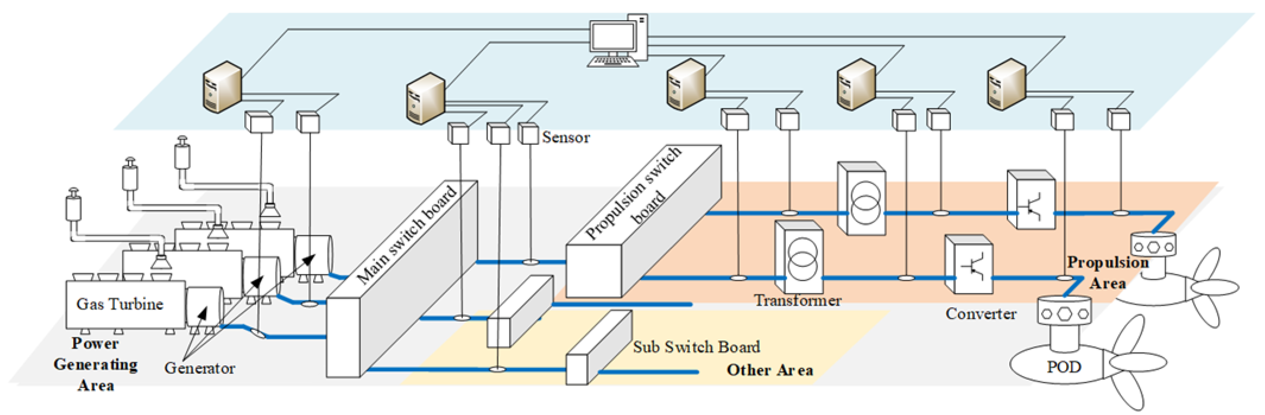
Modern ships are developing in the direction of large-scale, electrified, and intelligent. Electric propulsion has gradually replaced traditional heat engine propulsion and has become the preferred main power system for various ships today. The electrical structure of the port side power unit of an electric propulsion ship is shown in Figure 1. The power system of a large, intelligent ship generally adopts a regional power distribution scheme to support the operation of the electric propulsion system of an all-electric ship [17]. The scheme divides the ship’s load into multiple areas, such as propulsion area, living area, and important load, according to function and the degree of importance. Power is supplied by multiple gas turbines in the power generation area. The integrated power system monitors and evaluates the operation status of each area through sensor data. On the basis of ensuring the continuous and effective operation of the electric propulsion system, unified management and control of the electrical equipment of the whole ship are carried out according to the actual situation of navigation. As the main power unit of the ship, the propulsion system directly affects the safety of the ship during the voyage and needs to be given more attention.

The entire port side propulsion area is composed of a propulsion power distribution panel, an isolation transformer, a high-power drive inverter, a propulsion control system composed of a propulsion motor, and a monitoring system composed of sensors, computers, and servers. The propulsion system obtains stable electrical energy from the ship’s power generation unit through the propulsion power distribution panel and the transformer and drives the inverter to adjust the speed of the propulsion motor according to the command of the bridge telegraph to control the torque output of the propulsion system so that the ship can obtain forward power. Node sensor data, use computers to realize intelligent evaluation of propulsion system operating status and upload the results through the server so that the integrated power system can be managed in a unified manner.

For the long-term heavy-load operation of the system under harsh working conditions during the voyage, the marine electric propulsion system has high requirements for stability and reliability, and each device in the system needs to have a certain fault tolerance capability to gain time for the implementation of self-healing and maintenance strategies. Avoid system crashes. Therefore, an accurate fault diagnosis method is required to achieve rapid fault classification and provide data support for fault tolerance and maintenance strategy formulation. This paper takes the six-phase motor drive unit of the marine electric propulsion system as the research object and conducts fault diagnosis research on the IGBT open-circuit fault in the inverter circuit in the torque control mode.

2.1. Mathematical Model of Six-Phase Propulsion Motor

The ship’s six-phase propulsion unit is composed of a six-phase propulsion motor and a six-phase drive inverter. Compared with the traditional three-phase motor, the six-phase permanent magnet synchronous motor has obvious advantages in torque ripple, magnetomotive force waveform, and motor efficiency, and the multi-phase structure has the ability to realize high-power drive on the one hand, and the redundant structure on the other hand. It enables fault-tolerant operation of the motor after phase failure and improves the overall reliability of the propulsion system [18]. Therefore, six-phase PMSM is favored in large ships, luxury cruise ships, and other occasions that require high performance and reliability. Its stator winding structure is shown in Figure 2.

The stator winding of the six-phase permanent magnet synchronous motor is composed of two sets of three-phase symmetrical windings (ABC&XYZ) connected by a Y-shaped connection.

To simplify the analysis, it is assumed that the six-phase PMSM is an ideal motor, and the basic equations of voltage and flux linkage in the natural coordinate system were obtained.

$$\{\begin{array}{l}{u}_{\mathrm{s}}=R_{\mathrm{s}}{i}_{\mathrm{s}}+\frac{\mathrm{d}}{\mathrm{dt}}{\psi }_{\mathrm{s}}\\ {\psi }_{\mathrm{s}}=L_{\mathrm{s}}{i}_{\mathrm{s}}+{\psi }_{\mathrm{f}}\mathcal{F}(\theta )\end{array}$$

(1)

where

$$L_{\mathrm{s}}=\left[\begin{array}{cccccc}{L}_{\mathrm{AA}}& L_{\mathrm{AB}}& L_{\mathrm{AC}}& L_{\mathrm{AX}}& L_{\mathrm{AY}}& L_{\mathrm{AZ}}\\ L_{\mathrm{BA}}& L_{\mathrm{BB}}& L_{\mathrm{BC}}& L_{\mathrm{BX}}& L_{\mathrm{BY}}& L_{\mathrm{BZ}}\\ L_{\mathrm{CA}}& L_{\mathrm{CB}}& L_{\mathrm{CC}}& L_{\mathrm{CX}}& L_{\mathrm{CY}}& L_{\mathrm{CZ}}\\ L_{\mathrm{XA}}& L_{\mathrm{XB}}& L_{\mathrm{XC}}& L_{\mathrm{XX}}& L_{\mathrm{XY}}& L_{\mathrm{XZ}}\\ L_{\mathrm{YA}}& L_{\mathrm{YB}}& L_{\mathrm{YC}}& L_{\mathrm{YX}}& L_{\mathrm{YY}}& L_{\mathrm{YZ}}\\ L_{\mathrm{ZA}}& L_{\mathrm{ZB}}& L_{\mathrm{ZC}}& L_{\mathrm{ZX}}& L_{\mathrm{ZY}}& L_{\mathrm{ZZ}}\end{array}\right]$$

(2)

$$u_{\mathrm{s}}={[u_{\mathrm{A}} u_{\mathrm{B}} u_{\mathrm{C}} u_{\mathrm{X}} u_{\mathrm{Y}} u_{\mathrm{Z}}]}^{\mathrm{T}}$$

(3)

$${\mathsf{\psi }}_{\mathrm{s}}={[{\psi }_{\mathrm{A}} {\psi }_{\mathrm{B}} {\psi }_{\mathrm{C}} {\psi }_{\mathrm{X}} {\psi }_{\mathrm{Y}} {\psi }_{\mathrm{Z}}]}^{\mathrm{T}}$$

(4)

$$i_{\mathrm{s}}={[i_{\mathrm{A}} i_{\mathrm{B}} i_{\mathrm{C}} i_{\mathrm{X}} i_{\mathrm{Y}} i_{\mathrm{Z}}]}^{\mathrm{T}}$$

(5)

$$\mathcal{F}(\theta )={[\cos {(\theta )}^{}\cos {(\theta -\frac{2\mathsf{\pi }}{3})}^{}\cos {(\theta +\frac{2\mathsf{\pi }}{3})}^{}\cos {(\theta -\frac{\mathsf{\pi }}{6})}^{}\cos {(\theta -\frac{5\mathsf{\pi }}{6})}^{}\cos {(\theta +\frac{\mathsf{\pi }}{2})}^{}]}^{\mathrm{T}}$$

(6)

For the convenience of control, the VSD coordinate transformation was used to obtain Equation (7)

$$\{\begin{array}{l}{u}_{\mathrm{dq}0}=R_{\mathrm{s}}{i}_{\mathrm{dq}0}+L_{\mathrm{dq}0} \cdot \frac{\mathrm{d}}{\mathrm{dt}}{i}_{\mathrm{dq}0}+\left[\begin{array}{c}-{\omega }_{\mathrm{e}}{L}_{\mathrm{q}}{i}_{\mathrm{q}}\\ {\omega }_{\mathrm{e}}(L_{\mathrm{d}}{i}_{\mathrm{d}}+{\psi }_{\mathrm{f}})\end{array}\right]\hfill \\ u_{\mathrm{xy}0}=R_{\mathrm{s}}{i}_{\mathrm{xy}0}+L_{\mathrm{xy}0} \cdot \frac{\mathrm{d}}{\mathrm{dt}}{i}_{\mathrm{xy}0}\hfill \end{array}$$

(7)

and the motion equation can be expressed by Equation (8)

$$T_{\mathrm{e}}=3p_{\mathrm{n}}{i}_{\mathrm{q}}[i_{\mathrm{d}}(L_{\mathrm{d}}-L_{\mathrm{q}})-{\psi }_{\mathrm{f}}]$$

(8)

Modern electric propulsion ships use high-power inverters to control the propulsion motor. On the one hand, the system control performance is improved. On the other hand, the overcurrent protection of the inverter circuit can eliminate the motor insulation damage caused by overvoltage or overcurrent. The broken bar fault of the motor rotor can be eliminated by the soft start of the inverter, which greatly reduces the failure rate of the motor body [19]. Therefore, this paper mainly analyzes the failure of the switching device of the frequency conversion unit in the propulsion system and does not involve the failure of the motor itself.

2.2. Main Circuit Topology Structure and Failure Mode Classification

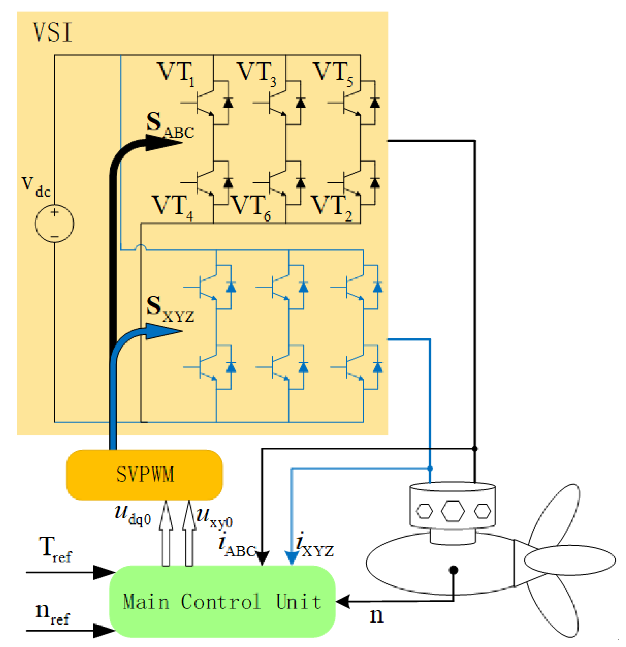
The six-phase motor of the ship is generally powered by two sets of three-phase two-level voltage source inverters (VSI). It can be seen from Equation (8) that the motor torque control can be achieved by controlling the output current of the inverter, and its topology is shown in Figure 3. The main control unit is based on the bridge. Given the speed and torque command, the speed sensor, and the feedback data of each phase current sensor, the motor control signal was calculated by the PI control algorithm, and the three-phase decoupling SVPWM method was used to generate the switching signal of the IGBT device of each bridge arm of the inverter to control the motor speed and rotation. The torque is used to drive the propeller to propel the ship to sail.

A drive inverter is an important unit of the propulsion control system. During the entire operation process, the switch is in a high-frequency switching state, and the power device loss is extremely large. In addition, the environment of the ship’s engine room is harsh, and it is easy to damage the main circuit devices and cause open-circuit or short-circuit faults [20]. However, in the actual operation process, the overcurrent caused by the short-circuit fault will trigger the protection mechanism and disconnect the device, which will eventually appear as an open-circuit fault in the system; there are a few cases of three open circuits [21]. In addition, due to the variety of faults, considering that the two sets of windings of the six-phase motor are relatively independent and have similar control structures, this paper only discusses the single and double faults of the ABC winding inverter circuit. The failure phenomenon of the IGBT circuit breaker of the six-phase propulsion motor drive inverter is shown in Figure 4.

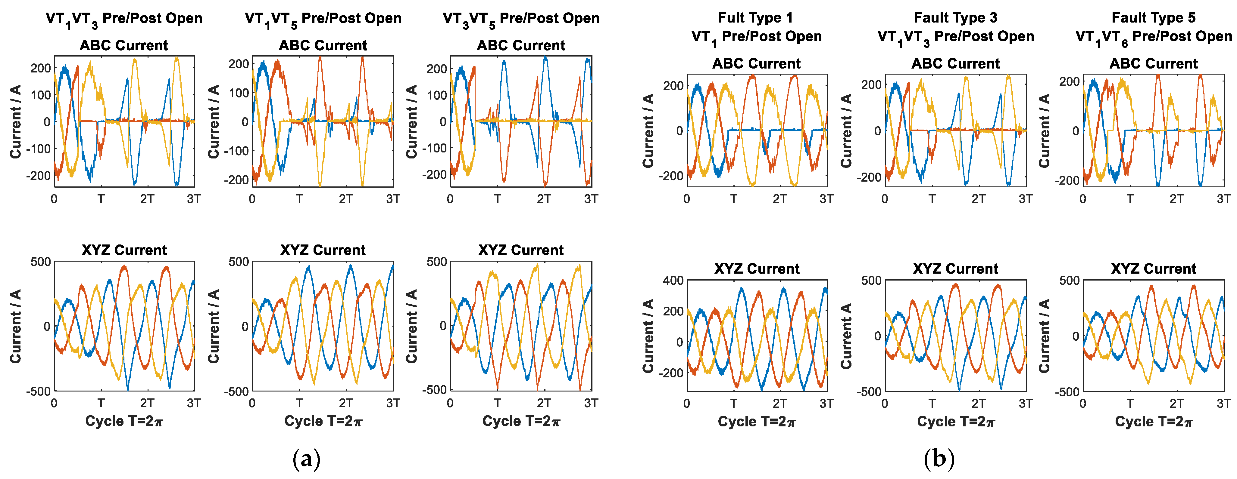
During the occurrence of a fault, the output six-phase current of the inverter will show different degrees of fault symptoms. The six-phase current waveforms of the same fault type are arranged in combination due to the fault phase sequence, while the six-phase current waveforms of different fault types are arranged according to the number of IGBT faults. It is different from the position of the faulty bridge arm and has a certain degree of randomness and uncertainty, so the collected current signal needs to be processed [22].

In addition, according to the current traces before and after the fault in Figure 5, it can also be seen that since the six-phase motor is controlled by two sets of three-phase inverters and the neutral point is isolated, the fault mainly affects the three-phase current of the same set of windings, and the current trace of the other set. Close to a circle, it will not cause the system to crash, which shows from the side that the system has fairly high fault tolerance.

According to these, 21 kinds of IGBT open-circuit faults are divided into six categories in

Table 1. Fault classification of inverter unit in marine electric propulsion system.

Label	Fault Type	Faulty Power Electronics
1	Upper Bridge Arm Single Transistor Open (UBAST)	VT1, VT3, VT5
2	Lower Bridge Arm Single Transistor Open (LBAST)	VT4, VT6, VT2
3	Same Side Upper Bridge Arm Double Transistor Open (SSUBADT)	VT1VT3, VT1VT5, VT3VT5
4	Same Side Lower Bridge Arm Double Transistor Open (SSLUBADT)	VT2VT4, VT2VT6, VT4VT6
5	Cross Side Bridge Arm Double Transistor Open (CSBADT)	VT1VT2, VT1VT6, VT3VT2, VT3VT4, VT5VT4, VT5VT6
6	Same Side Bridge Arm Double Transistor Open (SSBADT)	VT1VT4, VT3VT6, VT5VT2

for research.

3. Fault Diagnosis of Drive Inverter for Marine Electric Propulsion System Based on Res-BiLTM Deep Learning Method

The time-varying nonlinearity, stochastic uncertainty and the local observability of faults in marine electric propulsion systems make it difficult for traditional methods based on mathematical model analysis to fully reflect the fault characteristics, and the diagnostic effect is limited. Introducing artificial intelligence methods, such as deep learning, into the field of intelligent fault diagnosis, on the one hand, can alleviate the problems of mining massive current data and extracting fault features during electric propulsion system faults. On the other hand, it can make up for the lack of training data of traditional machine learning methods in practical applications, poor generalization ability, etc. The traditional shallow neural network has a certain degree of self-adaptation and robustness and has certain research results in the field of fault diagnosis. When dealing with fault diagnosis problems, the single traditional shallow neural network has limited ability to express nonlinear functions. When forecasting and other problems, underfitting is prone to occur [23].

To improve learning efficiency and performance, the concept of deep learning was introduced. Deep learning is based on a neural network. The network parameters were adjusted through training to obtain the weight value of each layer. Each layer represents a representation of the input data so as to convert the original data into the simplest representation. By constructing multiple hidden layers, the machine learning model and massive training data can be used to learn more useful features so as to improve the accuracy of classification and prediction. In fault diagnosis, the recognition-based deep learning model is generally used for fault classification, which can be characterized by the posterior distribution of the predicted class of the labeled data. The common convolutional neural network (CNN) was used in this paper to improve the accuracy of fault classification. The network analyzes the data time series to obtain the time-series correlation between the data, uses the pattern classification and pattern discrimination capabilities of the recognition model, and combines the two characteristics to form a deep learning network framework to improve the accuracy of fault classification.

3.1. The Structure of Convolutional Neural Network and Residual Network

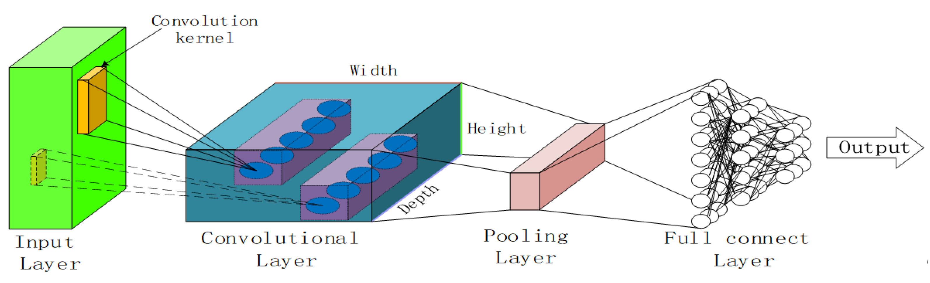
The convolutional neural network refers to a neural network that uses convolution operation instead of ordinary matrix penalty operation in at least one layer of the network and completes the extraction of local features of the original image through convolution and pooling operations. It is widely used in image classification, object detection, and other machine vision fields [24]. In fault diagnosis, CNN is usually regarded as a feature extractor composed of convolutional layers and pooling layers. It has the characteristics of local connection and weight sharing. It is a multi-layer supervised learning neural network for processing time-series data, which has a strong ability to deal with nonlinear problems. The typical CNN model mainly uses the convolution layer to perform the convolution operation (Convolution) to extract internal features; the pooling layer (Pooling) removes unnecessary information and improves the network generalization ability and calculation speed. The fully connected layer further abstracts and combines global time-series features and output, its structure is shown in Figure 6,

The convolution kernel extracts signal feature information through the special linear operation of convolution, which has the characteristics of sparse connection and weight sharing. The convolution kernel and the input signal are slid in a locally connected manner, and the eigenvalues of the signal were obtained by calculating the weight-sharing method during sliding. The calculation process is as follows:

$${\mathcal{F}}_i{}^{\mathrm{L}}=relu({\displaystyle \sum _i{x}_i^{\mathrm{L}}\ast w_{ij}^{\mathrm{L}}}+b_j^{\mathrm{L}})$$

(9)

where $\ast$ is the convolution operation, ${\mathcal{F}}_i{}^{\mathrm{L}}$ is the feature value extracted by the i-th channel in the L-th layer, $x^{\mathrm{L}}{}_i$ is the input of the i-th channel in the L-th layer, $w^{\mathrm{L}}{}_{ij}$ and $b_j^{\mathrm{L}}$ is the weight of the j-th convolution kernel in the corresponding layer and bias; the activation function $relu=\max (0,x)$ improves network sparsity by zeroing out some of the outputs.

The pooling layer is usually connected after the convolutional layer, and the downsampling operation is used to reduce the size of the feature data and network parameter space. In order to suppress the over-fitting phenomenon, this paper adopts the global pooling operation. The mathematical description is as follows:

$$P_i{}^{\mathrm{L}}=\frac{1}{\mathrm{k}}{\displaystyle \sum _{i=(j-1)\mathrm{k}+1}^{j\mathrm{k}}{a}_i^{\mathrm{L}}}$$

(10)

where $a_i^{\mathrm{L}}$ is the activation value of the i-th feature in the L-th layer, $P_i^{\mathrm{L}}$ is its corresponding value in the pooling layer, and k is the width of the pooling region. Alternating convolution and pooling processes can make the features extracted by the CNN from the input signal more discriminative and robust.

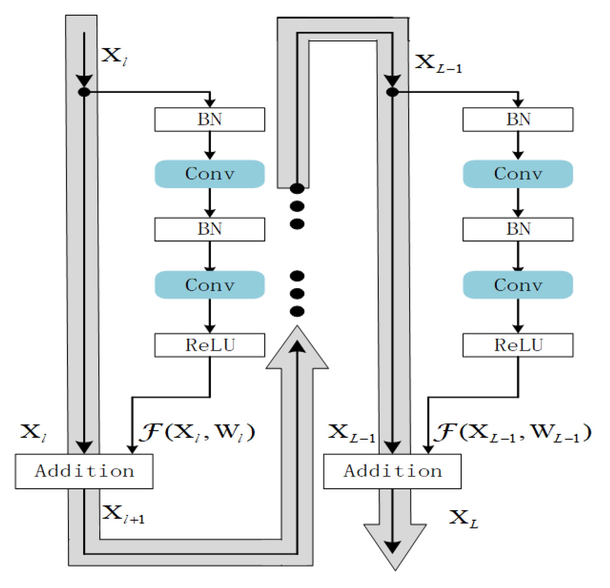
A deep network is a typical deep learning model, and its essence is a function chain; that is, each function is a layer, each layer is composed of neurons, and the neurons are connected by weights and biases. During DNN training, weights and biases are determined by minimizing the loss function on the dataset to avoid DNN overfitting [25]. Therefore, in principle, the network can learn more feature information and improve the training effect by increasing the convolutional layer and pooling layer in the CNN. However, in practical applications, it is found that too many convolutional layers will not only cause the gradient disappearance problem during the model training process but also increase the amount of calculation and increase the training time and hardware burden. Focusing on the problem of gradient disappearance in the stacking of locked layers of the convolutional neural network, this paper introduces the idea of residual error, adopts the residual network to retain the powerful fault feature extraction ability of CNN, and alleviates the problem of network degradation caused by the too deep network. Its structure is shown in Figure 7.

Figure 7 is a residual network, which can be mathematically expressed as

$$\{\begin{array}{l}{\mathrm{Y}}_l=h({\mathrm{X}}_l)+\mathcal{F}({\mathrm{X}}_l,{\mathrm{W}}_l)\\ {\mathrm{X}}_{l+1}=f({\mathrm{Y}}_l)\end{array}$$

(11)

Assuming that h is a linear mapping, f is a direct mapping, and $\mathcal{F}({\mathrm{X}}_L,{\mathrm{W}}_L)$ is the output of the number of convolutional networks, the output of the lth layer can be written as Equation (12).

$${\mathrm{X}}_{l+1}={\lambda }_l{\mathrm{X}}_l+\mathcal{F}({\mathrm{X}}_l,{\mathrm{W}}_l)$$

(12)

For a residual network of depth L, the Lth layer can be written as the sum of the residual parts between any shallow layers,

$${\mathrm{X}}_L=({\displaystyle \sum _{i=l}^{L-1}{\lambda }_i}{)\mathrm{X}}_l+{\displaystyle \sum _{i=l}^{L-1}\mathcal{F}({\mathrm{X}}_i,{\mathrm{W}}_i)}$$

(13)

Then the gradient of its loss function $\mathsf{\epsilon }$ with ${\mathrm{X}}_l$ respect to can be expressed as

$$\frac{\partial \mathsf{\epsilon }}{\partial {\mathrm{X}}_l}=\frac{\partial \mathsf{\epsilon }}{\partial {\mathrm{X}}_L}[{\displaystyle \prod _{i=l}^{L-1}{\lambda }_i}+\frac{\partial }{\partial {\mathrm{X}}_l}{\displaystyle \sum _{i=l}^{L-1}\mathcal{F}({\mathrm{X}}_i,{\mathrm{W}}_i)}]$$

(14)

From the analysis of Equation (14), it can be seen that if ${\lambda }_i>1$, it will lead to ${\displaystyle \prod _{i=l}^{L-1}{\lambda }_i}\to \infty$, and ${\lambda }_i<1$ will appear ${\displaystyle \prod _{i=l}^{L-1}{\lambda }_i}\to 0$, to avoid the situation of gradient explosion or gradient disappearance during the training process, we set ${\lambda }_i=1$. So, the new gradient can be expressed as Equation (15)

$$\frac{\partial \mathsf{\epsilon }}{\partial {\mathrm{X}}_l}=\frac{\partial \mathsf{\epsilon }}{\partial {\mathrm{X}}_L}[1+\frac{\partial }{\partial {\mathrm{X}}_l}{\displaystyle \sum _{i=l}^{L-1}\mathcal{F}({\mathrm{X}}_i,{\mathrm{W}}_i)}]$$

(15)

Considering that $\frac{\partial }{\partial {\mathrm{X}}_l}{\displaystyle \sum _{i=l}^{L-1}\mathcal{F}({\mathrm{X}}_i,{\mathrm{W}}_i)}$ is not always equal to 0, there will be no gradient disappearance problem in the residual. At the same time, due to the effect of the constant 1, the gradient of the L-th layer can be directly transferred to any shallow layer, realizing the information interaction between the high-level and low-level layers.

It can be seen from the analysis for Equations (11)–(15) that the residual structure of direct mapping has two structural advantages: first, when the network propagates forward, the shallow features can be reused in the deep layer; second, deep gradients can be directly passed back to the shallow layers when the network is back-propagated. Therefore, with a residual block, when there is a large reconstruction error between the input and output of the network, the error information can be directly fed back to the previous network layer through a shortcut connection. This structural design can also alleviate the model training speed without improving the network degradation problem.

3.2. Bidirectional Long Short-Term Memory Network

In the marine electric propulsion system, the output current of the drive inverter is affected by the integral link of the PI current controller, and its variation law is related to time and has a time sequence attribute. RNN is proposed for time series data. There are both internal feedback and feedforward connections between its neurons. The feedback connection can preserve the state of the hidden layer nodes of the network and provide a memory method. The network output is the result of the joint action of the current input and all historical states. It has certain advantages for time series processing, but the gradient dispersion effect on the time axis makes RNN unsuitable for processing long sequence data [26]. The Long Short-Term Memory (LSTM) network is a special recurrent neural network (RNN), which is a deep learning network optimized to solve the problem of gradient disappearance and gradient explosion during production sequence training. With the development of RNN, LSTM has excellent processing ability for sequence data and can retain the time-series features in current signals to the greatest extent so that it can be tried and applied in fault diagnosis in different fields. Different from the simple cell structure of the conventional RNN, three special ‘gate’ structures are added to the LSTM neurons so that the state information can be added or lost so that the state can flow with the sequence and the ability to obtain memory. The cell structure of LSTM is shown in the figure. “Gate” is a method to allow information to pass through. LSTM realizes memory by introducing forget gate, input gate, and output gate to control the state of cells. The LSTM memory cell structure is shown in Figure 8.

The forget gate selects the historical information to be retained according to the input $x_t$ at the t moment and the memory state $h_{t-1}$ of the previous moment; the input gate determines the content of the new information contained in the long-term memory state $c_t$; and the output gate controls the information contained in the long-term state $c_{t-1}$, which is passed to the next as short-term memory. Time and update the hidden state $h_t$. The internal calculation formula of the neuron is as follows:

$$\{\begin{array}{l}{f}_t=\sigma (W_f{h}_{t-1}+U_f{x}_t+b_f)\hfill \\ i_t=\sigma (W_i{h}_{t-1}+U_i{x}_t+b_i)\hfill \\ a_t=\tanh (W_a{h}_{t-1}+U_a{x}_t+b_a)\hfill \\ o_t=\sigma (W_o{h}_{t-1}+U_o{x}_t+b_o)\hfill \\ c_t=c_{t-1}{f}_t+i_t{a}_t\hfill \\ h_t=o_t\tanh (c_t)\hfill \end{array}$$

(16)

where, $\sigma (·)\in (0,1)$ is the sigmoid function, $\tanh (·)\in (-1,1)$ is the hyperbolic tangent function, $W$ and $U$ is the weight between the gates, and $b$ is the bias.

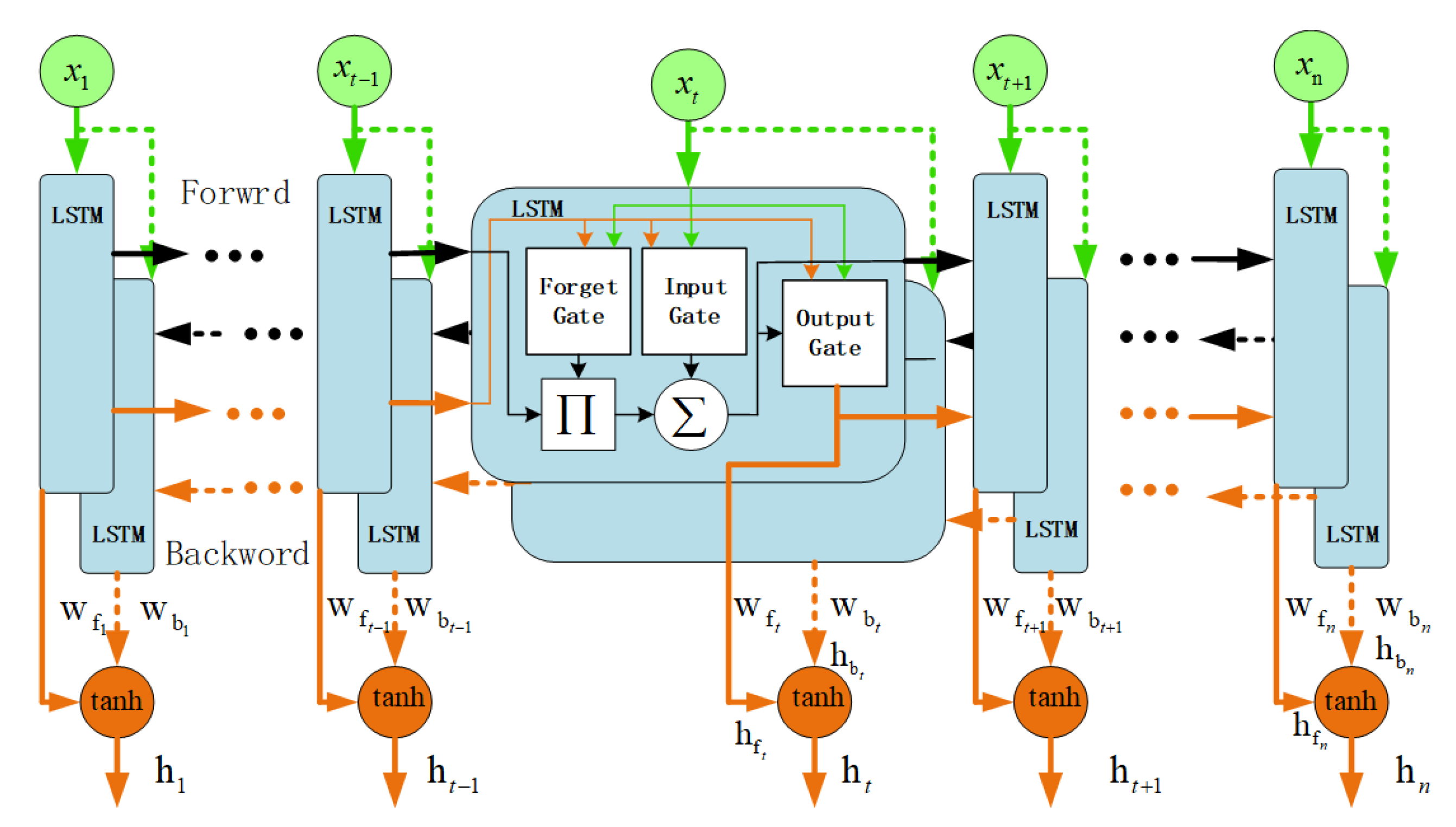
BiLSTM is a variant algorithm of LSTM. It consists of two layers of LSTM, one for forward propagation and one for reverse propagation. The forward layer starts the input iteration from the beginning of the sequence, the reverse layer starts the input iteration from the end of the sequence, and the output results of the two layers are combined to obtain the identification result. The state memory and transmission process are shown in Figure 9.

Its output ${\mathrm{y}}_t=\tanh ({\mathrm{W}}_{b_t}{h}_{b_t}+{\mathrm{W}}_{f_t}{h}_{f_t})$, ${\mathrm{W}}_{b_t}$ and ${\mathrm{W}}_{f_t}$ is the weight of the output layer in the output mapping of the forward layer and the reverse layer. Bidirectional LSTM can simultaneously learn the future and past sequence data at the current time point and can effectively extract the time series features of the data sequence. Therefore, BiLSTM inherits the memory ability of RNN for time series data. At the same time, based on LSTM, it not only overcomes the problem that long-term historical signals cannot be transmitted to the current moment but also can better extract the time series in fault current signals due to the addition of the reverse layer information to improve the performance of the diagnostic model

3.3. Fault Diagnosis Model of Marine Electric Propulsion Drive Inverter Based on Res-BiLSTM

The marine electric propulsion system has been in a noisy and time-varying working condition for a long time. The collected current signal is a non-stationary signal and contains noise. If the original current signal is directly input into the deep learning network for learning, it will affect the anti-interference ability of the diagnostic model. Therefore, the engineering is usually preprocessed by wavelet packet transform [27,28]. Using the compactness of the wavelet basis function, the original current signal is represented by a small number of wavelet coefficients as signal features, and the multi-feature overall evaluation is used to avoid one-sided blindness and reduce the randomness and uncertainty of the fault signal. Wavelet packet transform has the characteristics of time-frequency localization and high resolution. It can retain most of the original signal features and is highly sensitive to faults [29]. To avoid diagnostic errors caused by the artificial selection of features, the data after wavelet packet transformation are deeply excavated using the Res-BiLSTM deep learning framework to improve the diagnostic effect.

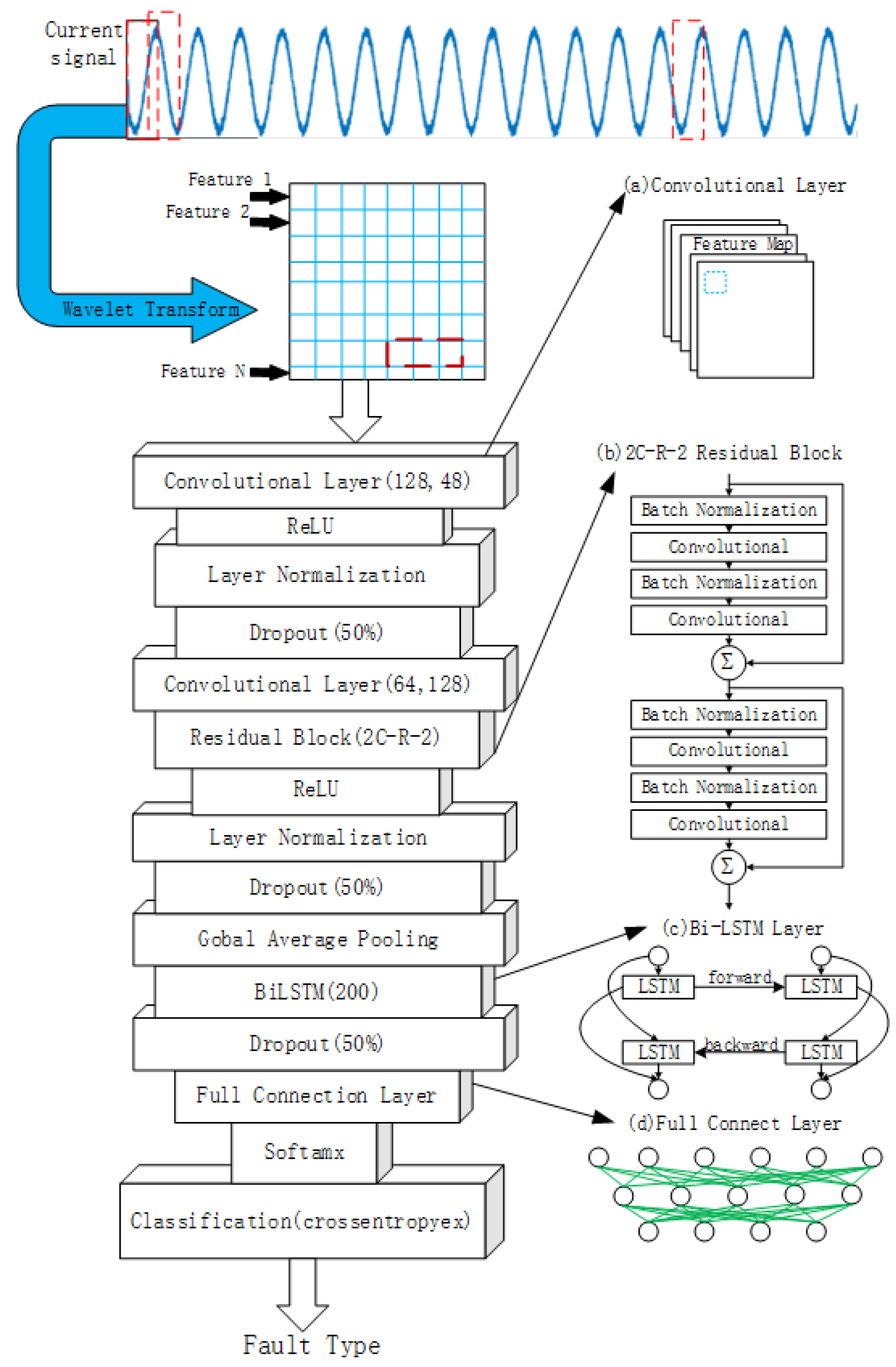
Considering the powerful fault feature extraction ability of CNN, ResNet formed by connecting CNN layers through residuals can extract deeper fault features and better capture the attribute information of fault occurrence; BiLSTM has long- and short-term memory ability and can capture the time sequence of fault occurrence information. Therefore, in order to obtain more attribute characteristics of fault signals and preserve the time-series characteristics of current signals to the greatest extent, this paper integrates the advantages of the two networks and designs a deep residual network integrating residual module and BiLSTM as a fault diagnosis model for ship electric propulsion drive units, which can not only extract the fault attribute information but also integrate the time sequence information of the fault into the fault diagnosis model, so as to improve the accuracy of the diagnosis results. The Res-BiLSTM network structure is shown in Figure 10, which includes two initial convolutional layers, a pooling layer, a bidirectional long short-term memory network layer, and two residual modules. BiLSTM layers are designed for temporal feature extraction, multilayer residual blocks are designed for deep fault feature extraction, and the global average pooling layers are designed to process the learned features, which treat each feature map as a region to perform the pooling operation and output the features to the classifier for fault classification, and finally output the fault label.

In the model, the first convolutional layer adopts a 3D convolutional neural network, the filter size is 128, and the convolution kernel size is 3. In the second convolutional layer, the filter size is 64, and the convolution kernel size is unchanged. In the global average pooling operation, the pooling block size is 3. The dropout is the discarding layer, and the discarding rate is 50%. The forward network and the reverse network in the bidirectional long-term memory layer each contain 100 neurons. ReLU means Rectified linear unit activation function and uses the Softmax classifier to classify multiple faults. The residual network is composed of two residual blocks in series. Two CNNs are connected by residuals to form a residual block. The convolutional layer of the CNN network extracts the local features of the upper-layer input neuron data and uses the convolution kernel to perform the feature map of the previous layer. The convolution calculation outputs a new feature map, which is used for data dimensionality reduction through the pooling layer, and input to the BiLSTM layer for time series feature learning to improve the performance of the diagnostic model.

4. Results Verification and Analysis of the Res-BiLSTM Fault Diagnosis Method

4.1. Training Process

Aiming at the problems of the complex and changeable working conditions of the marine electric propulsion system and the difficulty in extracting the special fault diagnosis caused by the strong nonlinearity of the fault current signal, this paper proposes a fault diagnosis method for marine electric propulsion drive based on the characteristics of the residual network and BiLSTM network. Based on the deep learning framework, the six-phase propulsion system model is established in the Matlab/Simulink environment, and the 30–100% torque fault and normal operating state are simulated in the cruise mode. Preprocess and divide the dataset and input it into the diagnostic model for learning and testing. The propulsion system parameters and Res-BiLSTM hyperparameters are shown in

Table 2. Parameters for Propulsion System and Hyper Parameters for Res-BiLSTM.

Propulsion System Parameter	Value	Hyper Parameter	Value
$\mathrm{Maximum}\mathrm{speed}{\mathrm{n}}_{\max }(\mathrm{r}/\min )$	170	Learning rate	0.0001
$\mathrm{Maximum}\mathrm{torque}{\mathrm{T}}_{\max }(\mathrm{N})$	205	Maximum iterations	10,000
$\mathrm{Pole\; number}\mathrm{p}$	8	Convolution Kernel Size	3
$\mathrm{Inertia}\mathrm{J}(\mathrm{kg}·{\mathrm{m}}^2)$	0.1	Hidden Units	200
$\mathrm{Stator}\mathrm{resistance}{\mathrm{R}}_{\mathrm{s}}(\Omega )$	0.01	Batch Size	22
$\mathrm{Stator}\mathrm{inductance}\mathrm{L}\left(\mathrm{mH}\right)$	2.4	State Activation Function	tanh
$\mathrm{Flux}{\mathsf{\psi }}_{\mathrm{s}}(\mathrm{Wb})$	0.04	Gate Activation Function	sigmoid
$\mathrm{IGBT}\mathrm{switching}\mathrm{frequency}{\mathrm{f}}_{\mathrm{sw}}(\mathrm{kHz})$	10	Dropout	0.5
$\mathrm{Sampling}\mathrm{frequency}{\mathrm{f}}_{\mathrm{s}}\left(\mathrm{kHz}\right)$	200	Solver for training network	Adam

, and the training and diagnosis process is shown in Figure 11.

Collect a total of 7040 groups of drive inverter output currents in the normal state and under six faults and obtain the characteristics of each phase current in eight frequency bands through three-layer wavelet packet transformation. A total of 48 groups of eigenvectors constitute the original data set and then follow the 8:1:1 split training set, validation set, and test set.

In the training phase, firstly, initialize the network parameters, input the training set data into the network for training, and use the validation set to adjust the network parameters by the Adam optimization method. After obtaining satisfactory results, end the training and save the network parameters to obtain a fault diagnosis model. In the fault diagnosis stage, input the test set data into the model obtained by training and output the diagnosis result.

To evaluate the diagnostic performance, the accuracy, precision, recall, and F1 score can be determined as

$$\mathrm{Accuracy}=\frac{\mathrm{True}\mathrm{Postives}+\mathrm{True}\mathrm{Negatives}}{\mathrm{True}\mathrm{Postives}+\mathrm{True}\mathrm{Negatives}+\mathrm{False}\mathrm{Postives}+\mathrm{False}\mathrm{Negatives}}$$

(17)

$$\mathrm{Precision}=\frac{\mathrm{True}\mathrm{Postives}}{\mathrm{True}\mathrm{Postives}+\mathrm{False}\mathrm{Postives}}$$

(18)

$$\mathrm{Recall}=\frac{\mathrm{True}\mathrm{Postives}}{\mathrm{True}\mathrm{Postives}+\mathrm{False}\mathrm{Negatives}}$$

(19)

$$\mathrm{F}1\mathrm{Score}=\frac{2\times \mathrm{True}\mathrm{Postives}}{2\times \mathrm{True}\mathrm{Postives}+\mathrm{False}\mathrm{Postives}+\mathrm{False}\mathrm{Negatives}}$$

(20)

4.2. Analysis of Training Performance

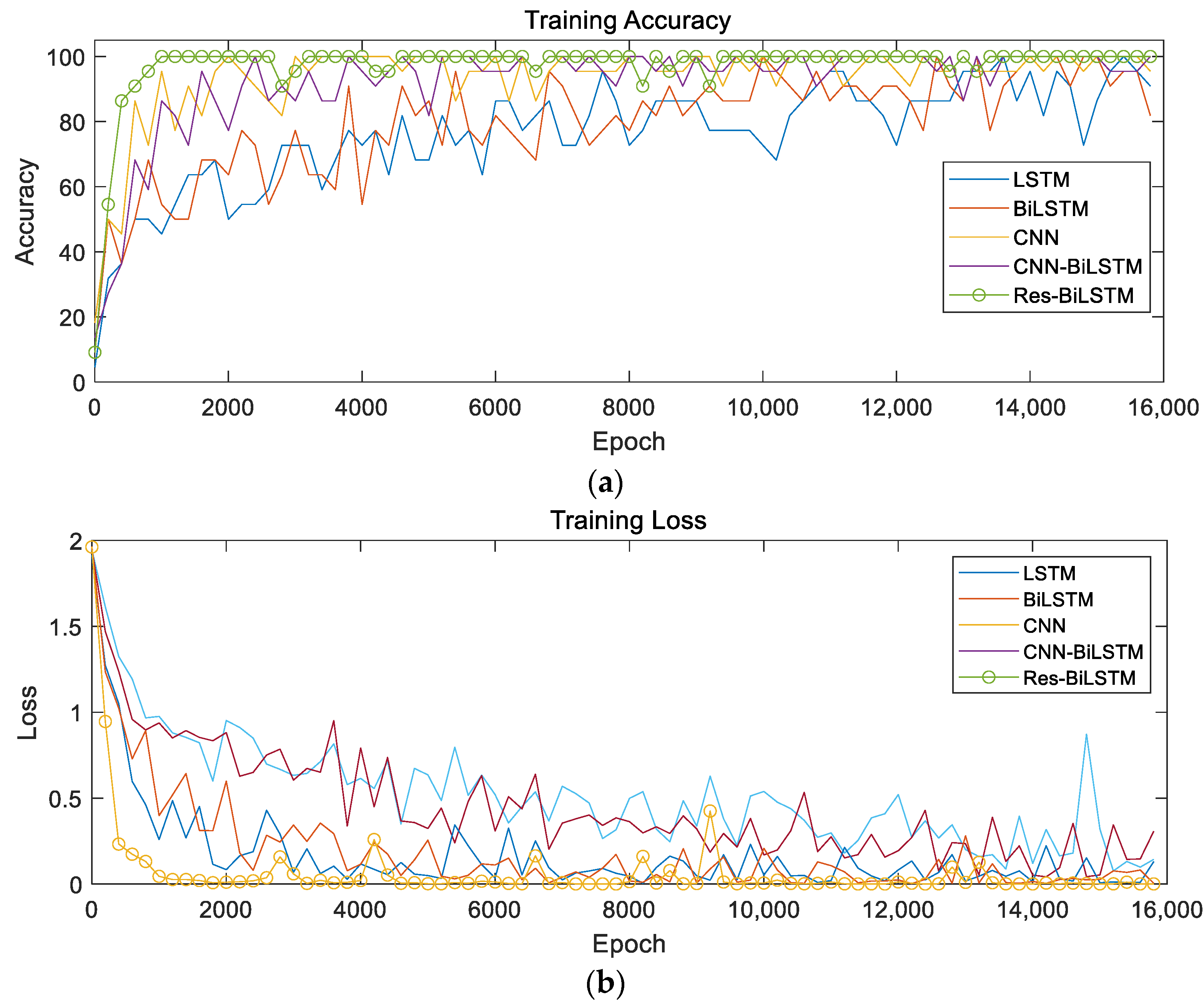
In the experiment, the existing deep learning model-based fault diagnosis methods LSTM, BiLSTM, CNN, and CNN-BiLSTM were used as the comparison models to compare with the Res-BiLSTM with the residual structure proposed in this paper. The training performance and comparison are shown in Figure 12.

The method proposed in this paper was superior to the other four deep learning methods in terms of training speed, accuracy, and loss function value. Combining the figures and figures, it can be seen that the learning speed was very fast in the first 500 times, and the training accuracy rate rose rapidly to 80%, 500 times. After the learning speed gradually slowed down, the training accuracy rate gradually stabilized above 95%, and in order to avoid overfitting, some features were discarded through the Dropout layer in each training so the accuracy rate would fluctuate slightly. The average training accuracy was 98.02%. The minimum loss function was 0.0554, the lowest loss function and the highest training effect, indicating that the Res-BiLSTM model obtained rich fault features through the residual network in the early stage of training, and the two-way LSTM was used to learn the time-series features of the fault features so that the training process was faster and more stable. The test set data was used to test the five trained networks to verify their fault diagnosis capabilities. The test results and confusion matrix are shown in Figure 13 and Table 2.

The multi-class confusion matrix contains both correct information and misclassified information. The position of the main diagonal represents the number of correct classifications for each fault. Above the main diagonal is the number of false classified data, and below the main diagonal is the misclassification. The number of data, 1–6 represents six different fault states, and 0 represents the normal state. From the confusion matrix of the four methods, BiLSTM can learn data time series features but cannot extract deeper fault features, resulting in high accuracy, but there are prediction errors and misclassifications in the results, and the CNN, with its powerful feature extraction ability of CNN-BiLSTM can obtain more fault attributes, but the ability to retain time-series features in the data is limited, so the prediction accuracy is improved, but there are still misclassifications, and CNN-BiLSTM combines the advantages of the two. The situation has been alleviated, and the Res-BiLSTM network strengthens its feature extraction ability through residual connection CNN, combined with the long and short-term memory ability of BiLSTM, and integrates its time-series information into the value model while extracting fault attribute information, and the diagnosis effect is further strengthened.

Analysis of

Table 3. Comparison of training performance of five learning frameworks.

	LSTM	BiLSTM	CNN	CNN-BiLSTM	Res-BiLSTM
Average Training Accuracy	76.32%	80.49%	92.60%	93.38%	98.02
Average Training Loss	0.5153	0.4322	0.1931	0.1777	0.0554
Testing Accuracy	87.07%	92.19%	96.45%	97.73%	100%

shows that BiLSTM has a good effect on fault identification, and the test accuracy rate can reach 92.19%, which is higher than that of the ordinary LSTM algorithm; the CNN-BiLSTM network composed of CNN and BiLSTM in series has an average training accuracy higher than that of the single network, reaching 93.38% Furthermore, it has an average test accuracy of 97.73%, which is higher than the effect of an independent diagnosis of the two networks, which proves that extracting feature vectors through CNN and then using the BiLSTM network for time series learning can effectively improve the identification accuracy. The Res-BiLSTM network using the residual connection proposed in this paper is the best in terms of training accuracy, loss function, and test accuracy, which proves that the CNN with a residual connection can perform deep learning on fault features and further improve the accuracy of fault diagnosis.

4.3. Robustness Analysis of Fault Classification Models

To verify the robustness of the fault classification model, the different intensities of noise were added to the test set and input into five diagnostic models. The performance results are shown in

Table 4. Accuracy comparison of different algorithms under different noises.

	25 dB	22 dB	20 dB	19 dB
LSTM	86.65	85.37	84.66	84.38
BiLSTM	90.48	87.93	87.64	87.07
CNN	95.31	90.63.	87.78	87.50
CNN-BiLSTM	97.44	94.60	93.61	93.34
Res-BiLSTM	98.58	98.15	96.02	95.03

.

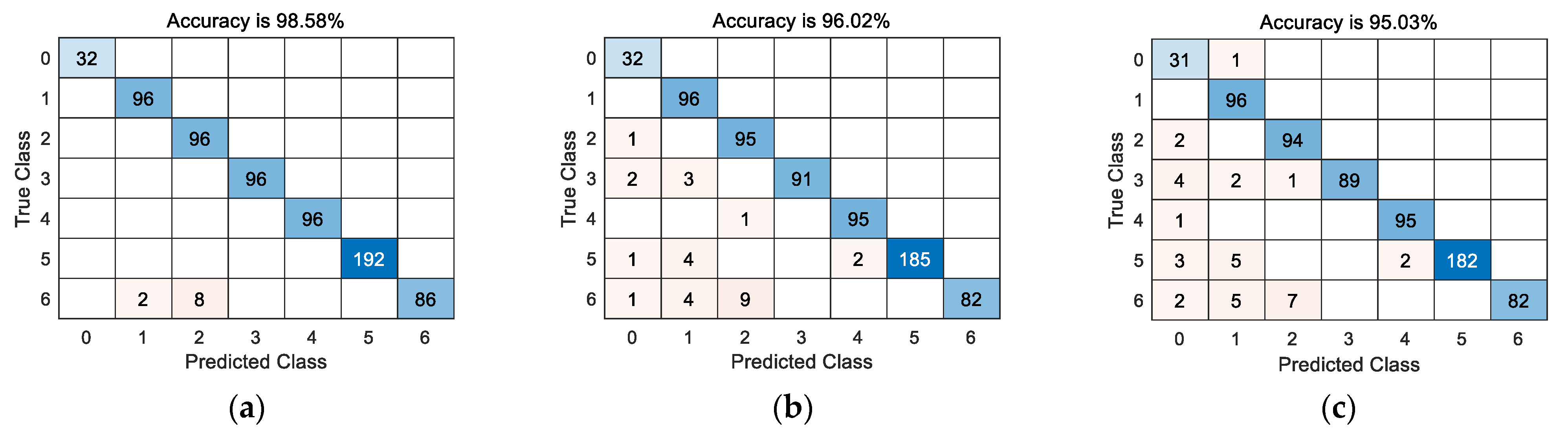
It can be seen that as the noise increases, the accuracy of the five diagnostic models decreases to varying degrees. With its powerful feature extraction capability, CNN can obtain enough fault feature attributes under noise interference, which can improve the correct classification results. Compared with CNN-BiLSTM, which simply increases the depth of the convolutional layer, Res-BiLSTM strengthens the fault characteristics of the network by connecting the convolutional layer through residuals. The extraction ability still has an accuracy of 95.03% under the condition of a 19 dB signal-to-noise ratio, indicating that the algorithm can ensure a high fault recognition rate in a high-noise environment.

Analyzing the confusion matrix under noise interference in Figure 14, it can be found that the powerful feature extraction ability of CNN makes the method proposed in this paper still have a high diagnostic accuracy in the case of noise, but some fault features are difficult to extract due to the influence of noise, and the test set. The data are unbalanced, and the number of different fault data is inconsistent, so some fault data are mistakenly identified as a normal state. Secondly, the double-pipe fault can be considered as the arrangement and combination of single-pipe faults, and its characteristics are similar. In a low-noise environment, the time series features can be extracted by BiLSTM to distinguish, but under the influence of high noise, the time series characteristics of the data are affected, and there is a situation in which a double-tube fault is mistakenly identified as a single-tube fault.

Observing the Res-BiLSTM in

Table 5. Comparison of Res-BiLSTM performance indexes under different noises.

Label	Fault Type	25 dB			20 dB			19 dB
		Precision	Recall	F1	Precision	Recall	F1	Precision	Recall	F1
0	Normal	100%	100%	100%	86.5%	100%	92.76%	72.1%	96.9%	82.68%
1	UBAST	98%	100%	98.99%	89.7%	100%	94.57%	88.1%	100%	93.67%
2	LBAST	93.2%	100%	96.48%	90.5%	99%	94.56%	92.2%	97.9%	94.96%
3	SSUBADT	100%	100%	100%	100%	94.8%	97.33%	100%	92.7%	96.21%
4	SSLBADT	100%	100%	100%	97.9%	99%	98.45%	97.9%	99%	98.45%
5	CSBADT	100%	100%	100%	100%	96.4%	98.17%	100%	94.8%	97.33%
6	SSBADT	100%	89.6%	94.51%	100%	85.4%	92.12%	100%	85.4%	92.12%

we can comprehensively evaluate the classification of various faults under different signal-to-noise ratios, and it can be found that the method in this paper still has a high index under a 19 dB noise interference, indicating that the proposed method is robust to noise. In addition, with the increase in noise content, the fastest decline in the precision is the normal situation, which is due to the small amount of normal data in the test set; that is, the data imbalance causes the classification results to be biased. However, in the case of false detection, the system will warn of non-existing faults, while missed detection will judge the fault condition as normal, which poses a potential safety hazard. In the actual situation, it is most important to ensure the safety of the ship’s navigation and prevent the occurrence of accidents. The missed detection under normal conditions has a more serious impact on the propulsion system than the false detection. From the recall rate of the normal operating conditions, it can be seen that the fault leakage under different levels of noise, the missed detection rate is lower than the false detection rate of less than 4%, so the proposed method can still have a good F1 score and fault classification effect. From Table 5, for the evaluation indicators under various noise conditions, the method in this paper can ensure a high fault recognition rate and a high evaluation so it can be used in the fault diagnosis of the inverter unit of the marine electric propulsion system.

5. Conclusions

To realize the self-healing of marine electric propulsion system faults, it is necessary to accurately classify the faults of the most fragile and complex motor drive units in the system. In this paper, a deep learning framework based on a residual network and bidirectional LSTM is proposed, which avoids manual filtering of fault features extracted by wavelet packets, and fully mines the feature attributes and timing characteristics of the fault signal, improving the learning efficiency and diagnosis effect. The simulation results show that the Res-BiLSTM deep learning method has the following characteristics:

• Realizing complex and high-dimensional function representation and providing an effective means of expressing features for fault data with complex features that are difficult to extract manually. It is beneficial to improve the feature expression of the intrinsic features of the state of the reaction system.
• Transferring the gradient to a deeper layer through the residual connection method, avoiding the disappearance of the gradient, thereby increasing the number of network layers, improving the generalization ability of the model, and reducing the computational complexity, the training effect is improved.
• Organically unifying the feature extraction and classification functions improves the performance of the algorithm and the robustness of the diagnostic model while increasing the diagnostic accuracy.

Combined with the above advantages, the Res-BiLSTM deep learning framework proposed in this paper can be used to establish a fault diagnosis model for the marine electric propulsion system to provide data support for self-healing decision-making, but the method still has the following shortcomings:

• The choice of deep learning network structure lacks a theoretical basis, and it is necessary to continue research on the deep learning algorithm itself.
• In the field of fault diagnosis, there is an imbalance between the number of fault samples and normal samples, which affects the training effect. Unsupervised learning does not require sample labels and can avoid problems caused by unbalanced sample proportions. Therefore, follow-up research will focus on how to combine the characteristics of existing unsupervised generative deep models to improve fault diagnosis models and realize discriminative unsupervised deep models.